A Godunov Method for Multidimensional Radiation Magnetohydrodynamics based on a variable Eddington tensor

Abstract

We describe a numerical algorithm to integrate the equations of radiation magnetohydrodynamics in multidimensions using Godunov methods. This algorithm solves the radiation moment equations in the mixed frame, without invoking any diffusion-like approximations. The moment equations are closed using a variable Eddington tensor whose components are calculated from a formal solution of the transfer equation at a large number of angles using the method of short characteristics. We use a comprehensive test suite to verify the algorithm, including convergence tests of radiation-modified linear acoustic and magnetosonic waves, the structure of radiation modified shocks, and two-dimensional tests of photon bubble instability and the ablation of dense clouds by an intense radiation field. These tests cover a very wide range of regimes, including both optically thick and thin flows, and ratios of the radiation to gas pressure of at least $10^{-4}$ to $10^{4}$. Across most of the parameter space, we find the method is accurate. However, the tests also reveal there are regimes where the method needs improvement, for example when both the radiation pressure and absorption opacity are very large. We suggest modifications to the algorithm that will improve accuracy in this case. We discuss the advantages of this method over those based on flux-limited diffusion. In particular, we find the method is not only substantially more accurate, but often no more expensive than the diffusion approximation for our intended applications.

1. Introduction

Moving fluids can absorb, emit and scatter photons, and via these processes energy and momentum are exchanged between the radiation field and the rest of the flow. When the fluxes of energy and momentum carried by photons are significant compared to those carried by particles or magnetic field, the fluid dynamics will be significantly affected (and perhaps even controlled) by the radiation field. Radiation has been realized to play an important role in the dynamics of many different astrophysical systems, such as the formation of stars in different environments (e.g., McKee & Ostriker, 2007; Krumholz et al., 2009; Offner et al., 2009; Jiang & Goodman, 2011), supernovae (e.g., Arnett et al., 1989; Janka et al., 2007; Nordhaus et al., 2010), accretion flows around supermassive massive black holes (e.g., Shakura & Sunyaev, 1973; Hirose et al., 2009; Spruit, 2010), and the evolution of galaxies with feedback from a central massive black hole (e.g., Ciotti & Ostriker, 2007; Proga, 2007), to name but a few.

The dynamics of radiating fluids can be divided into quite different regimes, depending on whether the photons dominate energy and/or momentum transport, and whether the optical depth across the region of interest is small or large (an excellent introduction to all aspects of radiation hydrodynamics is given in the monographs of Mihalas & Mihalas 1984 and Castor 2004). In this work, we are motivated by the properties of accretion flows around compact objects, the dynamics of accretion disk boundary layers, and the production of radiation-driven winds and outflows from stars, accretion disks, and galaxies. In these systems, radiation often dominates both the energy and momentum transport, and the optical depth can vary widely between different regions in the flow. Since magnetohydrodynamic (MHD) effects are crucial in accretion flows (see the review Balbus & Hawley, 1998, and references therein), they must be included. Thus, for these applications the appropriate equations are the those of gas dynamics, Maxwell’s equations, and the radiation transfer equation. Our goal is to develop numerical algorithms to solve this system of equations in order to investigate our motivating applications.

Although the basic equations of radiation MHD are well known, there is still considerable uncertainty regarding even fundamental issues of how to solve them. For example, it is not clear whether to treat the radiation field in the co-moving (fluid) or laboratory frame in order to obtain the simplest and most accurate solutions. Castor (2009) has provided a detailed critique of both approaches. In this work, we adopt the mixed frame (e.g., Mihalas & Mihalas, 1984), in which both the radiation and fluid variables are integrated in the laboratory frame, but the radiation-material interaction terms are treated in the co-moving frame, with $\mathcal{O}(v/c)$ expansions used to transform these terms back to the lab frame. A proper accounting of all $\mathcal{O}(v/c)$ terms in these transformations is necessary in order to correctly account for all effects (e.g., Lowrie et al., 1999; Krumholz et al., 2007). Although there are limitations to this approach (it is not suitable for treating line transport), we find it is well suited to our applications.

Rather than integrating the time-dependent transfer equation directly (which, even in the case of frequency independent transport, requires solving an integro-differential equation in 6 dimensions), we instead integrate a hierarchy of angular moments, using a variable Eddington tensor (VET) that relates the zeroth and second moments in order to close the system of equations. The VET is computed directly from a formal solution of the time-independent transfer equation at every time step. This approach has been implemented previously in both 2D and 3D versions of the ZEUS code (Stone et al., 1992; Hayes & Norman, 2003), the adaptive mesh refinement code TITAN (Gehmeyr & Mihalas, 1994) as well as a Soften Lagrangian Hydrodynamic code described in Gnedin & Abel (2001). However, because of the expense of solving the transfer equation in multidimensions, the VET method has not been widely used for astrophysical applications. Advances in algorithms and computer hardware now make the VET feasible even in 3D, and as we show in this paper, the VET method has considerable advantages over other methods. In a companion paper (Davis et al., 2012), we provide a detailed description of the algorithms we have implemented to solve the transfer equation.

A popular alternative to the VET method for closing the radiation moment equations is to adopt the flux-limited diffusion (FLD) approximation (e.g., Levermore & Pomraning, 1981). In this approach, the radiation flux is assumed to be in the direction of the gradient of the radiation energy density, with a value that is limited to prevent superluminal transport. In fact, the majority of multidimensional radiation hydrodynamic codes used in astrophysics to date adopt FLD (e.g., Turner & Stone, 2001; Krumholz et al., 2007; Gittings et al., 2008; Swesty & Myra, 2009; van der Holst et al., 2011; Commerçon et al., 2011; Zhang et al., 2011), However, there are a number of well-known and potentially serious limitations to FLD (e.g., Mihalas & Mihalas, 1984; Hayes & Norman, 2003). For example, the fact that the direction of the flux is assumed rather than computed from the transfer equation can introduce serious error in optically thin regions, such as the inability to follow shadows, or a net force on the fluid which is in the wrong direction. Dropping the time-dependent term in the radiation flux eliminates radiation inertia, which can be important when the radiation field carries a significant amount of the total momentum in the flow. Finally, in FLD the off-diagonal components of the radiation pressure tensor are dropped, which eliminates effects such as radiation viscosity. The VET method overcomes all of these limitations. We compare and contrast these two methods throughout this paper.

A significant difference between the algorithm developed in this paper and previous implementations of the VET method is the algorithm used to integrate the hydrodynamic (as well as the MHD) equations. Most previous implementations of VET used methods based on operator splitting, with artificial viscosity required for shock capturing as implemented in, for example, the ZEUS code (Stone et al., 1992). In this work we combine the VET approach with a dimensionally-unsplit higher-order Godunov method for hydrodynamics and MHD (as implemented in the Athena code, see Stone et al. 2008). By adopting a Riemann solver to compute fluxes of the conserved variables, Godunov methods do not require any artificial viscosity for shock capturing. However, a significant challenge to this approach is how to treat the stiff source terms associated with the interaction of the radiation and material. With Godunov methods, simply splitting these terms from the flux differences (the simplest and most often adopted approach) is known to be problematic when the source terms are stiff (e.g., Lowrie & Morel, 2001). Instead in this work we adopt the modified Godunov method of Miniati & Colella (2007), which provides a stable second-order accurate algorithm. In a previous paper Sekora & Stone (2010) (hereafter SS10), we introduced a one-dimensional version of this algorithm. This paper represents the multidimensional extension of the SS10 algorithm.

In addition to the modified Godunov method, a second crucial ingredient to the algorithm is the method by which the VET is computed. We use a formal solution of the radiative transfer (RT) equation based on the method of short characteristics, and including multi-frequency, scattering, and non-LTE effects. Angular quadratures of the specific intensity are then used to compute the VET from first principles. A complete description of our algorithm for solving the RT equation, including tests, is given in a companion paper (Davis et al., 2012). The RT module can also be used to compute images and spectra of MHD simulations for diagnostic purposes, and can even by used to compute the radiation source terms in the MHD equations for problems where only energy transport via photons is important. In effect, the algorithm described in this paper is a marriage between the modified Godunov method of SS10 (extended to multidimensions) and a modern non-LTE stellar atmospheres code to compute the VET.

Of course, the final measure of any algorithm is provided by quantitative testing. Unfortunately, there are very few analytic solutions available in radiation hydrodynamics and MHD useful for such tests. In this paper, we introduce a comprehensive test suite that includes error convergence tests of radiation-modified acoustic waves in a variety of regimes, quantitative comparison of the structure of radiating shocks in the non-equilibrium diffusion limit to semi-analytic solutions over a wide range of Mach numbers, quantitative comparison to previous numerical solutions of the structure of subcritical radiating shocks computed with full-transport, the linear growth rate and nonlinear regime of the photon bubble instability, and shadowing and ablation of dense clumps by an intense radiation field. It is likely that many of these tests will be useful for others developing radiation hydrodynamic codes.

The outline of this paper is as follows. In the next section, we catalog the equations of motion we solve. In section 3, we describe in detail our numerical algorithms, highlighting the extensions we have made to the 1D method described by SS10. In section 4, we discuss the importance of exact energy conservation, and present test problems to measure the energy error. We present the results of our comprehensive test suite in section 6. Finally, we compare and contrast our numerical algorithms to those based on the diffusion approximation in section 7, and summarize in section 8.

2. Equations

Following SS10, we write the equations of radiation MHD in the mixed frame, and solve the radiation and material energy and momentum conservation laws separately, including the $\mathcal{O}(v/c)$ source terms as given by Lowrie et al. (1999). Similar equations have also been derived by Krumholz et al. (2007) in the flux-limited diffusion approximation, and the source terms used here are identical to those in Krumholz et al. (2007) to $\mathcal{O}(v/c)$. Some important $(v/c)^{2}$ terms are also included in our formula, such as the advective flux of radiation enthalpy. See the discussions in Lowrie et al. (1999) on the importance of keeping these terms. We find it convenient to solve the system of equations in a dimensionless form by adopting the two ratios ${\mathbb{C}}=c/a_{0}$ and ${\mathbb{P}}=a_{r}T_{0}^{4}/P_{0}$. Here $a_{0}$, $T_{0}$, and $P_{0}$ are the characteristic values of sound speed, gas temperature, and gas pressure respectively, and $a_{r}$ is the radiation constant. Thus, ${\mathbb{C}}$ is the dimensionless speed of light, and ${\mathbb{P}}$ the dimensionless radiation pressure. With these scalings, the units of the radiation energy density and flux are $a_{r}T_{0}^{4}$ and $ca_{r}T_{0}^{4}$ respectively.

To further simplify the equations, we assume frequency-independent (gray) opacities, and local thermodynamic equilibrium (LTE). The scattering opacity is assumed to be isotropic and coherent in the co-moving frame. Thus, we only consider the equations for frequency-integrated quantities, and do not need to distinguish between Planck and flux-mean opacities. Extension of our method to frequency dependent transport problems, for example using multigroup methods (e.g., Vaytet et al., 2011), is straightforward but beyond the scope of this paper. The equations of radiation MHD are then:

$$\frac{\partial\rho}{\partial t}+{\mbox{\boldmath$\nabla$}}\cdot(\rho{\mbox{\boldmath$v$}}) = 0,$$

$$\frac{\partial(\rho{\mbox{\boldmath$v$}})}{\partial t}+{\mbox{\boldmath$\nabla$}}\cdot({\rho{\mbox{\boldmath$v$}}{\mbox{\boldmath$v$}}-{\mbox{\boldmath$B$}}{\mbox{\boldmath$B$}}+{{\sf P}^{\ast}}}) = -\mathbb{P}{\bf S_{r}}({\mbox{\boldmath$P$}}),\$$

$$\frac{\partial{E}}{\partial t}+{\mbox{\boldmath$\nabla$}}\cdot\left[(E+P^{\ast}){\mbox{\boldmath$v$}}-{\mbox{\boldmath$B$}}({\mbox{\boldmath$B$}}\cdot{\mbox{\boldmath$v$}})\right] = -\mathbb{PC}S_{r}(E),$$

$$\frac{\partial{\mbox{\boldmath$B$}}}{\partial t}-{\mbox{\boldmath$\nabla$}}\times({\mbox{\boldmath$v$}}\times{\mbox{\boldmath$B$}}) = 0,$$

$$\frac{\partial E_{r}}{\partial t}+\mathbb{C}{\mbox{\boldmath$\nabla$}}\cdot{\mbox{\boldmath$F$}}_{r} = \mathbb{C}S_{r}(E),$$

$$\frac{\partial{\mbox{\boldmath$F$}}_{r}}{\partial t}+\mathbb{C}{\mbox{\boldmath$\nabla$}}\cdot{\sf P}_{r} = \mathbb{C}{\bf S_{r}}({\mbox{\boldmath$P$}}),$$ (1)

where the source terms are,

$${\bf S_{r}}({\mbox{\boldmath$P$}}) = -\sigma_{t}\left({\mbox{\boldmath$F$}}_{r}-\frac{{\mbox{\boldmath$v$}}E_{r}+{\mbox{\boldmath$v$}}\cdot{\sf P}_{r}}{\mathbb{C}}\right)+\sigma_{a}\frac{{\mbox{\boldmath$v$}}}{\mathbb{C}}(T^{4}-E_{r}),$$

$$S_{r}(E) = \sigma_{a}(T^{4}-E_{r})+(\sigma_{a}-\sigma_{s})\frac{{\mbox{\boldmath$v$}}}{\mathbb{C}}\cdot\left({\mbox{\boldmath$F$}}_{r}-\frac{{\mbox{\boldmath$v$}}E_{r}+{\mbox{\boldmath$v$}}\cdot{\sf P}_{r}}{\mathbb{C}}\right).$$ (2)

In the above, $\rho$ is density, ${\sf P}^{\ast}\equiv(P+B^{2}/2){{\sf\boldmath I}}$ (with ${{\sf\boldmath I}}$ the unit tensor), $\sigma_{a}$ and $\sigma_{s}$ are the absorption and scattering opacities (which can be functions of both density and temperature), and the magnetic permeability $\mu=1$. The total gas energy density is

$$E=E_{g}+\frac{1}{2}\rho v^{2}+\frac{B^{2}}{2},$$ (3)

where $E_{g}$ is the internal gas energy density. We adopt an equation of state for an ideal gas with adiabatic index $\gamma$, thus $E_{g}=P/(\gamma-1)$ for $\gamma\neq 1$ and $T=P/R_{\text{ideal}}\rho$, where $R_{\text{ideal}}$ is the ideal gas constant. The radiation pressure ${\sf P}_{r}$ is related to the radiation energy density $E_{r}$ by the closure relation

$${\sf P}_{r}={\sf\boldmath f}E_{r}.$$ (4)

where ${\sf\boldmath f}$ is the VET. It is straightforward to convert the dimensionless radiation MHD equations given above to their more familiar dimensional form by setting ${\mathbb{P}}=1$, and replacing ${\mathbb{C}}$ with the speed of light $c$, $T^{4}$ with $a_{r}T^{4}$, and ${\mbox{\boldmath$F$}}_{r}$ with ${\mbox{\boldmath$F$}}_{r}/c$.

The VET used to close the hierarchy of radiation moment equations is calculated directly from angular quadratures of the frequency averaged specific intensity $I_{r}$

$${\sf\boldmath f}=\frac{{\sf P}_{r}}{E_{r}}=\frac{\oint I_{r}\hat{\mathbb{n}}\hat{\mathbb{n}}d\omega}{\oint I_{r}d\omega},$$ (5)

where $\omega$ is solid angle and $\hat{\mathbb{n}}$ is the unit vector. The specific intensity $I_{r}$ is calculated from a formal solution of the time-independent transfer equation

$$\frac{\partial I_{r}}{\partial s}=\kappa_{t}(S-I_{r}),$$ (6)

where $\kappa_{t}$ is the total specific opacity and $S$ the source function. In a companion paper (Davis et al., 2012), we describe in detail the algorithm we use to solve the transfer equation 6, which is based on the method of short characteristics. In section 3.4, we describe how the angular quadratures of the specific intensity returned by the transfer solver are computed to give the Eddington tensor.

In the above equations, radiation quantities are always defined in the Eulerian (lab) frame. To order $\mathcal{O}(1/{\mathbb{C}})$, the co-moving radiation energy density $E_{r,0}$ and radiation flux ${\mbox{\boldmath$F$}}_{r,0}$ are related to the lab frame values $E_{r}$ and ${\mbox{\boldmath$F$}}_{r}$ by (e.g., Castor, 2004)

$$E_{r,0} = E_{r}-2\frac{{\mbox{\boldmath$v$}}}{\mathbb{C}}\cdot{\mbox{\boldmath$F$}}_{r},$$

$${\mbox{\boldmath$F$}}_{r,0} = {\mbox{\boldmath$F$}}_{r}-\frac{1}{\mathbb{C}}\left({\mbox{\boldmath$v$}}E_{r}+{\mbox{\boldmath$v$}}\cdot{\sf P}_{r}\right),$$

$$E_{r} = E_{r,0}+2\frac{{\mbox{\boldmath$v$}}}{\mathbb{C}}\cdot{\mbox{\boldmath$F$}}_{r,0},$$

$${\mbox{\boldmath$F$}}_{r} = {\mbox{\boldmath$F$}}_{r,0}+\frac{1}{\mathbb{C}}\left({\mbox{\boldmath$v$}}E_{r,0}+{\mbox{\boldmath$v$}}\cdot{\sf P}_{r,0}\right).$$ (7)

The source terms (equation 2) in the mixed frame representation were originally developed by Mihalas & Klein (1982), and extended by Lowrie et al. (1999) to include an extra term $(\sigma_{a}-\sigma_{s}){\mbox{\boldmath$v$}}\cdot({\mbox{\boldmath$v$}}E_{r}+{\mbox{\boldmath$v$}}\cdot{\sf P}_{r})/{\mathbb{C}}^{2}$ in the energy source term $S_{r}(E)$. This term is necessary to ensure the correct thermal equilibrium state in moving fluids, and is especially important when scattering opacity is dominant (see a full discussion in Lowrie et al. 1999). Further discussion of the physical interpretation of the source terms can be found in Section 7.1.

We do not solve the equations in strong conservation form, which means that total (radiation plus gas) energy and momentum are not conserved exactly (to round-off error). However, exact conservation is easily enforced only for explicit algorithms, in which case the time step is limited by the light crossing time across a cell. Once implicit differencing methods are adopted, then conservation to round-off error is generally not possible due to the much larger error tolerance used when inverting the matrix representing the difference equations. Since the use of implicit methods is crucial in our application domain, we choose to solve the radiation and material conservation laws with source terms as accurately as possible, and monitor the energy error as a diagnostic. The issue of the importance of exact energy conservation is discussed in more detail, along with results of tests of energy conservation in our methods, in section 4.

3. Numerical Algorithm

In a previous paper (SS10) we presented a one-dimensional modified Godunov algorithm for radiation hydrodynamics. In this paper our focus will be on the additional extensions and improvements to the SS10 method required in multidimensions. The numerical algorithms described in this paper have been implemented in the Athena MHD code (Stone et al., 2008). Athena implements higher-order reconstruction in the primitive variables, an extension of a dimensionally unsplit integrator to MHD, the constrained transport (CT) algorithm to enforce the divergence-free constraint on the magnetic field, and a variety of approximate and exact Riemann solvers. Since comprehensive descriptions of the algorithms in Athena has been given previously (Stone et al., 2008), in this section we only describe the extensions to these algorithms necessary for radiation MHD.

One challenge to any numerical algorithm for radiation MHD is the large range of timescales. In our applications, we are interested in evolving the system on the sound crossing time, which can be many orders of magnitude larger than the light crossing time. Thus, implicit differencing methods are essential. In this work, to improve both stability and accuracy, we split an implicit solution of the radiation subsystem from a modified explicit update of the rest of the equations. That is, we update the radiation energy density $E_{r}$ and flux ${\mbox{\boldmath$F$}}_{r}$ by solving the moment equations

$$\frac{\partial E_{r}}{\partial t}+\mathbb{C}{\mbox{\boldmath$\nabla$}}\cdot{\mbox{\boldmath$F$}}_{r} = \mathbb{C}S_{r}(E),$$

$$\frac{\partial{\mbox{\boldmath$F$}}_{r}}{\partial t}+\mathbb{C}{\mbox{\boldmath$\nabla$}}\cdot{\sf P}_{r} = \mathbb{C}{\bf S_{r}}({\mbox{\boldmath$P$}}).$$ (8)

using fully implicit, backward Euler differencing. As discussed in SS10, higher-order implicit time integration schemes can lead to oscillatory solutions with large time steps. Thus, to ensure a non-oscillatory method, we restrict the update to first-order backward Euler. During this step, the gas variables in the source terms $S_{r}(E)$ and ${\bf S_{r}}({\mbox{\boldmath$P$}})$ are held constant.

On the other hand, the gas quantities are updated by solving the ideal MHD equations using a time-explicit modified Godunov algorithm for the stiff source terms

$$\frac{\partial\rho}{\partial t}+{\mbox{\boldmath$\nabla$}}\cdot(\rho{\mbox{\boldmath$v$}}) = 0,$$

$$\frac{\partial(\rho{\mbox{\boldmath$v$}})}{\partial t}+{\mbox{\boldmath$\nabla$}}\cdot({\rho{\mbox{\boldmath$v$}}{\mbox{\boldmath$v$}}-{\mbox{\boldmath$B$}}{\mbox{\boldmath$B$}}+{\sf P}^{\ast}}) = -\mathbb{P}{\bf S_{r}}({\mbox{\boldmath$P$}}),\$$

$$\frac{\partial{E}}{\partial t}+{\mbox{\boldmath$\nabla$}}\cdot\left[(E+P^{\ast}){\mbox{\boldmath$v$}}-{\mbox{\boldmath$B$}}({\mbox{\boldmath$B$}}\cdot{\mbox{\boldmath$v$}})\right] = -\mathbb{PC}S_{r}(E),$$

$$\frac{\partial{\mbox{\boldmath$B$}}}{\partial t}-{\mbox{\boldmath$\nabla$}}\times({\mbox{\boldmath$v$}}\times{\mbox{\boldmath$B$}}) = 0.$$ (9)

In this step, the radiation variables are held constant. Note that the source terms themselves are not split from the flux-divergence terms. This is critical for achieving stable and accurate solutions when the source terms are stiff.

The order in which we do these updates is arbitrary. In most cases, we update the gas dynamical variables (that is, equations 9) first. However, when the the radiation pressure is completely negligible, we have found switching the order of the update is more robust.

3.1. Basic Steps in the Algorithm

To begin with, it is useful to summarize all of the individual steps in the overall algorithm:

Step 1.— Using the gas variables to compute the opacities and source function, solve the transfer equation over a large set of angles using short characteristics, and compute the Eddington tensor ${\sf\boldmath f}$.

Step 2.— Reconstruct the left- and right-states in the primitive variables at cell interfaces along each of the $x$, $y$, and $z$ directions independently. We reconstruct the primitive variables, instead of the conserved variables as in SS10, since we have found it to be less oscillatory and more accurate. Either second- or third-order spatial reconstruction is possible.

Step 3.— Add the radiation energy and momentum source terms to the left and right states (see equations 79 and 80 in SS10). Source terms for the left (right) states are calculated by using cell-centered quantities from the cell to the left (right) of the interface, and use the modified Godunov method.

Step 4.— Compute 1D fluxes of the conserved variables with the appropriate Riemann solver. For radiation hydrodynamic simulations, we use the HLLC solver, while for radiation MHD simulations we generally use HLLD. We use the adiabatic sound speed (instead of the radiation modified sound speed as was used by SS10) to calculate the fluxes. This adds extra dissipation and makes the algorithm more robust. We do not calculate fluxes for $E_{r}$ and ${\mbox{\boldmath$F$}}_{r}$ because they are not updated in this step; therefore the Riemann solvers are the same as those described in Stone et al. (2008).

Step 5.— For radiation MHD calculations, use constrained transport (CT) algorithm, (step 3 of the Athena 3D algorithm) to calculate the electric field at cell corners and update the face centered magnetic field.

Step 6.— Evolve the left- and right-states at each interface with the transverse flux gradients for half time step $\Delta t/2$, as required for the unsplit CTU integrator in Athena.

Step 7.— For radiation MHD calculations, calculate the cell-centered electric field at time $t^{n+1/2}$ to use as a reference state in CT algorithm (step 6 of the Athena 3D algorithm).

Step 8.— Calculate new fluxes along each direction with the corrected left- and right-states and the appropriate Riemann solver.

Step 9.— Update the area averaged magnetic field at cell faces from time step $n$ to $n+1$ using CT (step 8 of Athena 3D algorithm).

Step 10.— Update the gas variables from time $n$ to $n+1$ by adding the divergence of the flux gradient and the source terms using the modified Godunov method.

Step 11.— Estimate the value of radiation energy source term added to the gas total energy using the method described in Section 3.3.1. Then update the radiation variables $E_{r},\ {\mbox{\boldmath$F$}}_{r}$ using fully implicit, backward Euler differencing of the radiation moment equations 8. This requires solving a large linear system in multidimensions. Gas variables do not change during this step.

Step 12.— Update the time $t^{n+1}=t^{n}+\Delta t$, calculate the new time step according to the CFL condition with the adiabatic sound speed (fast magnetosonic speed) for radiation hydrodynamics (MHD).

In comparison to the algorithm introduced in SS10, the primary changes we have made to extend the scheme to multidimensions are in Step 1 (compute the Eddington tensor in multidimensions), Step 2 (reconstruction in the primitive rather than conserved variables), Step 11 (using an estimate of the radiation energy source term, and solving the implicit moment equations in multidimension), and Step 12 (choose a timestep based on the adiabatic sound speed).

3.2. Modified Godunov Method in Multidimensions

In this subsection, we describe in detail the modified Godunov method to calculate the flux, especially the way to add the stiff source terms to the left and right states.

3.2.1 Reconstruction Step

To compute the left- and right-states of the vector of conserved variables required to calculate the fluxes via a Riemann solver, we reconstruct the primitive variables as originally proposed by Miniati & Colella (2007), instead of the conserved variables (SS10). In hydrodynamics, the primitive and conserved variables are related via

$$\footnotesize\left(\begin{array}[]{c}\rho\\ v_{x}\\ v_{y}\\ v_{z}\\ P\end{array}\right)=\left[\begin{array}[]{ccccc}1&0&0&0&0\\ 0&1/\rho&0&0&0\\ 0&0&1/\rho&0&0\\ 0&0&0&1/\rho&0\\ (\gamma-1)(v_{x}^{2}+v_{y}^{2}+v_{z}^{2})/2&-(\gamma-1)v_{x}&-(\gamma-1)v_{y}&-(\gamma-1)v_{z}&\gamma-1\end{array}\right]\left(\begin{array}[]{c}\rho\\ \rho v_{x}\\ \rho v_{y}\\ \rho v_{z}\\ E\end{array}\right).$$ (10)

The radiation source terms for velocity and pressure are

$${\bf S_{r}}({\mbox{\boldmath$v$}}) = -{\mathbb{P}}{\bf S_{r}}({\mbox{\boldmath$P$}})/\rho$$ (11)

$$S_{r}(P) = (\gamma-1){\mathbb{P}}{\mbox{\boldmath$v$}}\cdot{\bf S_{r}}({\mbox{\boldmath$P$}})-(\gamma-1){\mathbb{P}}{\mathbb{C}}S_{r}(E),$$

where ${\bf S_{r}}({\mbox{\boldmath$P$}})$ and $S_{r}(E)$ are given by equation 2. These source terms are the same in the case of radiation MHD, even though in this case the definition of total gas energy $E$ includes the magnetic energy. Either second- or third-order reconstruction schemes can be used (Stone et al., 2008).

The radiation source terms for the primitive variables must be added to the left- and right-states for one half time step. This requires calculating the propagation operator $\mathcal{I}$ to project off the unstable mode (e.g., Miniati & Colella, 2007, SS10), using the gradient of radiation source terms on the plane of primitive variables ${\mbox{\boldmath$\nabla$}}_{W}{\bf S_{r}}({\mbox{\boldmath$W$}})$. As discussed in SS10, in most cases it is the energy source term $S_{r}(E)$ (or equivalently $S_{r}(P)$) that defines the stiffness of the problem. The momentum source term can be added as a normal body force. However, in the extreme case of radiation pressure so large that ${\mathbb{P}}\gtrsim{\mathbb{C}}$, the momentum source term may also become stiff. For example, this can happen in the inner regions of an accretion disk around a supermassive black hole, where ${\mathbb{C}}\sim 10^{2}$ while ${\mathbb{P}}\sim 10^{2}$ (e.g., Shakura & Sunyaev, 1973; Turner et al., 2003). For this reason, we keep the leading term in the momentum source term, so ${\mbox{\boldmath$\nabla$}}_{W}S_{r}({\mbox{\boldmath$W$}})$ can be written as

$${\mbox{\boldmath$\nabla$}}_{W}{\bf S_{r}}({\mbox{\boldmath$W$}})=\left(\begin{array}[]{ccccc}0&0&0&0&0\\ 0&S^{v_{x}}_{v_{x}}&0&0&0\\ 0&0&S^{v_{y}}_{v_{y}}&0&0\\ 0&0&0&S^{v_{z}}_{v_{z}}&0\\ S^{P}_{\rho}&S^{P}_{v_{x}}&S^{P}_{v_{y}}&S^{P}_{v_{z}}&S^{P}_{P}\end{array}\right),$$ (12)

where $S^{x}_{y}\equiv\partial S_{r}(x)/\partial y$ for any quantity $x$ and $y$.

For example, in the $x$-direction $S^{P}_{v_{x}}/S^{P}_{P}\sim\mathcal{O}(v/{\mathbb{C}}^{2})$ and $S^{P}_{v_{x}}/S^{P}_{\rho}\sim\mathcal{O}(v/{\mathbb{C}}^{2})$. To order $v/{\mathbb{C}}$, we can take $S^{P}_{v_{x}}=S^{P}_{v_{y}}=S^{P}_{v_{z}}=0$, which significantly simplifies the analysis (a significant advantage of using the primitive variables). Then the propagation operator is

$${\sf\mathcal{I}}\left(\frac{\Delta t}{2}\right) = \frac{1}{\Delta t/2}\int_{0}^{\Delta t/2}e^{\tau{\mbox{\boldmath$\nabla$}}_{W}{\bf S_{r}}\left({\mbox{\boldmath$W$}}\right)}d\tau$$ (18)

$$= \left(\begin{array}[]{ccccc}1&0&0&0&0\\ 0&\beta_{x}&0&0&0\\ 0&0&\beta_{y}&0&0\\ 0&0&0&\beta_{z}&0\\ (\alpha-1)S^{P}_{\rho}/S^{P}_{P}&0&0&0&\alpha\end{array}\right)$$

$$\approx \left(\begin{array}[]{ccccc}1&0&0&0&0\\ 0&\beta_{x}&0&0&0\\ 0&0&\beta_{y}&0&0\\ 0&0&0&\beta_{z}&0\\ (1-\alpha)P/\rho&0&0&0&\alpha\end{array}\right),$$ (24)

where we define the following quantities

$$\beta_{x} = \left[\text{exp}(S^{v_{x}}_{v_{x}}\Delta t/2)-1\right]/(S^{v_{x}}_{v_{x}}\Delta t/2),$$

$$\beta_{y} = \left[\text{exp}(S^{v_{y}}_{v_{y}}\Delta t/2)-1\right]/(S^{v_{y}}_{v_{y}}\Delta t/2),$$

$$\beta_{z} = \left[\text{exp}(S^{v_{z}}_{v_{z}}\Delta t/2)-1\right]/(S^{v_{z}}_{v_{z}}\Delta t/2),$$

$$\alpha = \left[\text{exp}(S^{P}_{P}\Delta t/2)-1\right]/(S^{P}_{P}\Delta t/2).$$ (25)

Note that $S^{v_{x}}_{v_{x}}$, $S^{v_{y}}_{v_{y}}$, $S^{v_{z}}_{v_{z}}$ $\sim\mathcal{O}(-\sigma_{t}{\mathbb{P}}/{\mathbb{C}})$ and when $\sigma_{t}{\mathbb{P}}/{\mathbb{C}}\ll 1$, then $\beta_{x},\ \beta_{y},\ \beta_{z}\approx 1$. In this case the propagation operator is reduced to the form used in SS10. When $\sigma_{t}{\mathbb{P}}/{\mathbb{C}}\gg 1$, then $\beta_{x}$, $\beta_{y}$ and $\beta_{z}$ ensure that the algorithm is still stable in this regime. With this propagation operator, the source terms added to the left- and right-states are $0.5\Delta t\times{\sf\mathcal{I}}(\Delta t/2){\bf S_{r}}({\mbox{\boldmath$W$}})$.

3.2.2 Fluxes from the Riemann Solver

Once the left- and right-states are calculated with the appropriate radiation source terms added, the fluxes of the conserved variables in each direction can be calculated from any of the Riemann solvers currently implemented in Athena (e.g., HLLC for radiation hydro, and HLLD for radiation MHD). Unlike SS10, the characteristic speed uses in those solvers is not the radiation modified sound speed (equation 73 of SS10), but the adiabatic sound speed. We have found this is necessary to make the multidimensional algorithm stable at a CFL number of 1.0 in 2D, and 0.5 in 3D (the same stability limits for the extension of the CTU integrator to MHD without radiation).

In radiation MHD, the cell-centered electromotive force (EMF) must be calculated as a reference state in the CT algorithm after we get the above fluxes (step 5 of the 2D integrator and step 6 of 3D integrator in Stone et al. 2008). In this step, momentum needs to be evolved for a half time step and radiation source terms ${\bf S_{r}}({\mbox{\boldmath$P$}})$ need to be added.

In the multidimensional CTU integrator, the left- and right-states must be corrected with the transverse flux gradients. Because the radiation subsystem is only first order accurate, transverse gradients of the source terms do not need to be added. This is done in the same way as in Athena (equation 86 and 87 of Stone et al. 2008). Using the corrected left- and right-states, we call the Riemann solver again to calculate the fluxes, which are then used in the following predict-correct step.

3.2.3 Updating the conserved variables with the predict-correct scheme

To achieve second-order accuracy, the conserved variables in this step are updated with a predict-correct scheme, similar to the approach taken by Miniati & Colella (2007) and SS10. The radiation quantities (energy and flux) have already been updated by the implicit solution of the radiation subsystem, so they are kept constant during this step. To be consistent with our reconstruction step, the stiffness of the momentum source terms in some regions must also be taken into account.

Given the divergence of the fluxes (computed as described above) ${\mbox{\boldmath$\nabla$}}\cdot{\mbox{\boldmath$F$}}^{n+1/2}$ and the radiation source term ${\bf S_{r}}({\mbox{\boldmath$U$}}^{n})$, a predict solution is estimated as

$$\hat{{\mbox{\boldmath$U$}}}={\mbox{\boldmath$U$}}^{n}+\Delta t({{\sf\boldmath I}}-\Delta t{\mbox{\boldmath$\nabla$}}_{U}{\bf S_{r}}({\mbox{\boldmath$U$}}^{n}))^{-1}\left({\bf S_{r}}({\mbox{\boldmath$U$}}^{n})-{\mbox{\boldmath$\nabla$}}\cdot{\mbox{\boldmath$F$}}^{n+1/2}\right),$$ (26)

where ${\mbox{\boldmath$\nabla$}}_{U}{\bf S_{r}}({\mbox{\boldmath$U$}}^{n})$ is the gradient of the radiation source term ${\bf S_{r}}({\mbox{\boldmath$U$}})$ with respect to the conserved variables ${\mbox{\boldmath$U$}}^{n}$ as

$${\mbox{\boldmath$\nabla$}}_{U}{\bf S_{r}}({\mbox{\boldmath$U$}})=\left(\begin{array}[]{ccccc}0&0&0&0&0\\ 0&S^{M_{x}}_{M_{x}}&0&0&0\\ 0&0&S^{M_{y}}_{M_{y}}&0&0\\ 0&0&0&S^{M_{z}}_{M_{z}}&0\\ S^{E}_{\rho}&S^{E}_{M_{x}}&S^{E}_{M_{y}}&S^{E}_{M_{z}}&S^{E}_{E}\end{array}\right).$$ (32)

The error in this predicted solution, $\epsilon(\Delta t)$, is estimated as

$$\epsilon(\Delta t)={\mbox{\boldmath$U$}}^{n}+\frac{\Delta t}{2}\left({\bf S_{r}}({\mbox{\boldmath$U$}}^{n})+{\bf S_{r}}(\hat{{\mbox{\boldmath$U$}}})\right)-\Delta t{\mbox{\boldmath$\nabla$}}\cdot{\mbox{\boldmath$F$}}^{n+1/2}-\hat{{\mbox{\boldmath$U$}}}.$$ (33)

Then the correction step is

$${\mbox{\boldmath$U$}}^{n+1}=\hat{{\mbox{\boldmath$U$}}}+({{\sf\boldmath I}}-\Delta t{\mbox{\boldmath$\nabla$}}_{U}{\bf S_{r}}({\mbox{\boldmath$U$}}^{n}))^{-1}\epsilon(\Delta t).$$ (34)

At the end of this step, all gas and radiation quantities are updated to time step $n+1$, and the entire algorithm can be repeated in the next cycle.

3.3. Radiation Subsystem in Multidimensions

In this subsection, we describe the extensions to SS10 required to integrate the radiation subsystem equations 8 in multidimensions.

3.3.1 Special Treatment of the energy source term

The radiation energy density $E_{r}$ and flux ${\mbox{\boldmath$F$}}_{r}$ are updated from time step $n$ to $n+1$ based on the updated gas quantities at time step $n+1$, using first-order backward Euler time differencing to make the method stable with a time step much larger than the light crossing time. However, in SS10, the source terms on the right hand side of equations 8 were calculated using the temperature at time step $n$. We have found this can introduce significant error in the total energy when the gas and radiation are far from thermal equilibrium, and the time step is much bigger than the thermalization time. The source of this error is the assumption that the gas temperature is constant during the update and thus the energy source terms added to the gas energy density and radiation energy density are not the same. This will be worse if there is continuous heating or cooling source terms and the energy error may accumulate. In reality, the gas temperature should evolve simultaneously with the radiation energy density until thermal equilibrium is reached.

To reduce this energy error, we first estimate the change of gas energy density due to the radiation energy source term in the modified Godunov step. Let ${\mbox{\boldmath$\nabla$}}\cdot{\mbox{\boldmath$F$}}^{n+1/2}$ be the Riemann flux calculated in Section 3.2.2. The updated gas total energy after the Godunov step is $E^{n+1}$ and the gas total energy at the beginning of the step is $E^{n}$. Then the change of gas energy due to the radiation energy source term in this step $dS_{r}(E)$ can be estimated as

$$dS_{r}(E)=E^{n+1}-(E^{n}-dt{\mbox{\boldmath$\nabla$}}\cdot{\mbox{\boldmath$F$}}^{n+1/2}).$$ (35)

To conserve total energy, the energy source term added to the radiation subsystem is then $\tilde{S}_{r}(E)=\mathcal{R}\left({\mathbb{C}}\sigma_{a}(\tilde{T}^{4}-E_{r})+(\sigma_{a}-\sigma_{s}){\mbox{\boldmath$v$}}\cdot\left({\mbox{\boldmath$F$}}_{r}-({\mbox{\boldmath$v$}}E_{r}+{\mbox{\boldmath$v$}}\cdot{\sf P}_{r})/\mathbb{C}\right)\right)-(1-\mathcal{R})dS_{r}(E)/(dt{\mathbb{P}})$, where the estimated temperature $\tilde{T}^{4}=-(1/(dt{\mathbb{C}}\sigma_{a})+1)dS_{r}(E)/{\mathbb{P}}+E_{r}^{n}$. Here $\mathcal{R}$ is a parameter we can choose to get the best energy conservation. In practice, we find $\mathcal{R}=0.05$ can give the best results for the tests we have done.

With this special treatment of the energy source term in the radiation moment equations, we can reduce the energy error significantly, especially for states that are initially far from thermal equilibrium in optically thick regions that are evolved with a time step much larger than the thermalization time (in practice, such states are extremely rare in any dynamical evolution, and usually occur only if set up specifically in the initial conditions). However, we still cannot conserve total energy to round-off error. We present tests in section 4 that show in practice, the error in total energy conservation is small.

3.3.2 The 3D matrix

The generalization of the fully implicit, backward Euler update of the radiation moment equations to 3D is straightforward. For this step, the vector of conserved quantities at time step $n$ is ${\bf U}^{n}_{i,j,k}=(E_{r},F_{r,x},F_{r,y},F_{r,z})$ . The radiation flux $F_{r,x},F_{r,y},F_{r,z}$ are advanced to time step $n+1$ by solving

$${\bf U}_{i,j,k}^{n+1} = {\bf U}_{i,j,k}^{n}-\frac{\Delta t}{\Delta x}\left[{\bf F}^{HLLE}_{i+1/2,j,k}-{\bf F}^{HLLE}_{i-1/2,j,k}\right]-\frac{\Delta t}{\Delta y}\left[{\bf F}^{HLLE}_{i,j+1/2,k}-{\bf F}^{HLLE}_{i,j-1/2,k}\right]$$ (36)

$$- \frac{\Delta t}{\Delta z}\left[{\bf F}^{HLLE}_{i,j,k+1/2}-{\bf F}^{HLLE}_{i,j,k-1/2}\right]+\Delta t{\bf S}({\bf U}^{n+1}_{i,j,k}),$$

while the radiation energy density $E_{r}$ is updated as

$$E_{r,i,j,k}^{n+1} = E_{r,i,j,k}^{n}-\frac{\Delta t}{\Delta x}\left[{\bf F}^{HLLE}_{i+1/2,j,k}-{\bf F}^{HLLE}_{i-1/2,j,k}\right]-\frac{\Delta t}{\Delta y}\left[{\bf F}^{HLLE}_{i,j+1/2,k}-{\bf F}^{HLLE}_{i,j-1/2,k}\right]$$ (37)

$$- \frac{\Delta t}{\Delta z}\left[{\bf F}^{HLLE}_{i,j,k+1/2}-{\bf F}^{HLLE}_{i,j,k-1/2}\right]+\tilde{S}_{r}(E),$$

where the ${\bf F}^{HLLE}$ are the vector of fluxes for the conserved quantities at each cell interface computed by a HLLE Riemann solver (equation 39 in SS10) and $dS_{r}(E)$ is the estimate energy source term (equation 35). Since the backward Euler differencing is only first-order in time, first-order spatial reconstruction is used to compute the left- and right-states for the HLLE solver. Moreover, since both the HLLE fluxes and the source term ${\bf S}({\bf U}^{n+1})$ in equation 36 and 37 are linear in the unknowns ${\bf U}^{n+1}_{i,j,k}$, then only one matrix solve is required per time step, which can represent a significant savings compared to the implicit solution of nonlinear equations that can result from other splittings (e.g., Turner & Stone, 2001; González et al., 2007). The matrix of coefficients that must be inverted to solve the linear system in this step is given in Appendix A.

3.4. Computing the Eddington tensor

In order to calculate the VET, we use a formal solution of time-independent transfer equation 6. The methods for solving the radiative transfer equation are described in Davis et al. (2012), and the reader is referred to that work for further details. At each time step, and for each grid cell, the specific intensity $I_{r}$ must be integrated along many different rays $\hat{n}$. The angular discretization and corresponding quadratures are chosen to cover the unit sphere as uniformly as possible, but still be invariant under 90 degree rotations about the coordinate axes (e.g., Bruls et al., 1999). Along each ray, the method of short characteristics (e.g., Mihalas et al., 1978; Olson & Kunasz, 1987) is used to integrate the transfer equation across the entire mesh. For multidimensional problems, this requires the interpolation of intensities, opacities, and emissivities from (only) neighboring grid zones. Simulations with scattering opacity (non-LTE problems) are solved iteratively with accelerated lambda iteration, with methods similar to those described in Trujillo Bueno & Fabiani Bendicho (1995). Intensity boundary conditions and parallelization are handled via ghost zones, as described in section 3.5 of Davis et al. (2012).

During the integration along each angle, the zeroth moment ($J$) and second moment (${\sf K}$) of the specific intensity are summed into running quadratures. This saves having to allocate an array to store $I_{r}$ over all angles. For each discreet ray $\hat{n}_{k}$, there is a vector of direction cosines $(\mu_{0k},\mu_{1k},\mu_{2k})$ with $\mu_{ik}=\hat{n}_{k}\cdot\hat{x}_{i}$ and quadrature weights $w_{k}$. The moments are then given by

$$J = \sum_{k=0}^{n_{a}-1}w_{k}I_{k}$$ (38)

$$K_{ij} = \sum_{k=0}^{n_{a}-1}w_{k}I_{k}\mu_{ik}\mu_{jk},$$ (39)

where $I_{k}\equiv I_{r}(\hat{n}_{k})$. Up to a common factor of $4\pi/c$, $J$ and ${\sf K}$ are equivalent to radiation energy density and pressure, respectively. Since they are computed by the radiation transfer solver, they will (in general) differ from the $E_{r}$ and ${\bf P_{r}}$ of the integrator. As defined in equation (6), the VET is then simply the ratio of these quadratures ${\sf f}={\sf K}/J$, evaluated in each grid cell.

4. Evaluating the Importance of Exact Energy Conservation

As discussed in section 3.3, our algorithm does not conserve energy exactly (to round-off error), in part because we separate the implicit solution of the radiation subsystem from the modified Godunov update of the material conservation laws. In fact, even if the strong conservation form of the equations is adopted, it is in general not possible to conserve energy to round-off error with implicit differencing if an iterative method is used to solve the resulting linear system to some error criterion. Therefore, our philosophy is to monitor energy conservation as a measure of the accuracy of the solution, rather than adopting ad-hoc strategies to enforce conservation.

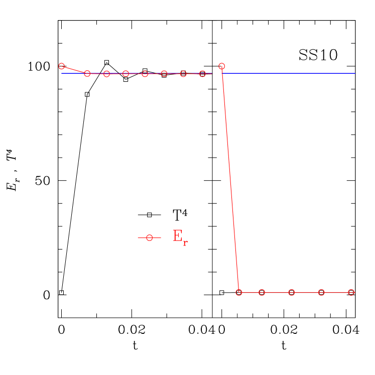
We have found that one important modification to the original algorithm described in SS10 that improves energy conservation is to estimate the energy source term added in the modified Godunov step and then use the same value of energy source term in the radiation subsystem (section 3.3.1). A test which demonstrates the importance of this improvement is thermal relaxation in a uniform, stationary medium. Consider an infinite uniform gas with density $\rho$, temperature $T$, and constant absorption opacity $\sigma_{a}$. The radiation energy density $E_{r}$ is also uniform everywhere and the radiation flux is zero. If the gas and radiation are not in thermal equilibrium, i.e. $E_{r}\neq T^{4}$ in our dimensionless units, then they will evolve towards the equilibrium state $\tilde{E_{r}}=\tilde{T}^{4}$ on the thermalization time scale $\sim P/({\mathbb{P}}E_{r}\sigma_{a}{\mathbb{C}})$ (e.g., Blaes & Socrates, 2003). The exact solution is set by the condition of energy conservation ${\mathbb{P}}E_{r}+\rho R_{\text{ideal}}T/(\gamma-1)={\mathbb{P}}\tilde{E_{r}}+\rho R_{\text{ideal}}\tilde{T}/(\gamma-1)$. We test this evolution using ${\mathbb{C}}=10^{4},{\mathbb{P}}=1,\rho=1,R_{\text{ideal}}=1,\gamma=5/3$ and $\sigma_{a}=100$, with different initial $T$ and $E_{r}$, in a domain of size $L=2$ and 128 grid points, and periodic boundary conditions. In our algorithm the time step is determined by the CFL condition using the adiabatic sound speed, which gives about $\sim 5\times 10^{-3}$, much larger than the thermalization time $\sim 10^{-6}$. This problem has also been used to test other codes (e.g., SS10, Zhang et al., 2011), but here we choose extreme values of the parameters in order to demonstrate potential problems. These values are almost certainly unrealistic in that no dynamical evolution could result in these conditions in any cell, but nevertheless it is useful.

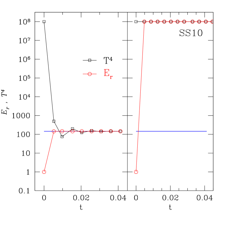
We show the solutions for two different initial conditions: $E_{r}=100,T=1$ (Figure 1) and $E_{r}=1,T=100$ (Figure 2) respectively. Results with our modifications are shown in the left panels of these figures, while the solutions given by the method used in SS10 are shown in the right panels. It is clear the our special treatment of the radiation energy source term reduces the error in the energy significantly, especially in the case when $E_{r}-T^{4}$ is very large. The right columns confirm the analysis in section 3.3.1, in that with the original method proposed by SS10, when the time step is much larger than thermalization time, $E_{r}$ approaches $T^{4}$ in a single step. Unfortunately, this is the wrong solution in the case that $E_{r}=1$ and $T=100$. Because our algorithm adds the same energy source term to the gas and radiation energy density, we conserve total energy much better. In this case, the energy error in our algorithm is determined by the tolerance level we set in the matrix solver. These tests also demonstrate stability even when the time step is much larger than the thermalization time.

Figure 1.— Evolution of the radiation and gas energies for relaxation to thermal equilibrium using a timestep $\sim 10^{3}$ larger than the thermalization time. The left panel is the result with our special treatment of the energy source term (section 3.3.1) while the right column is the result with the original method used by SS10. The red (black) lines are for $E_{r}$ ($T^{4}$) while the blue lines are the thermal equilibrium state.

Figure 2.— Same as figure 1, but with a different initial condition. Although the initial difference of $T^{4}-E_{r}$ is $\sim 10^{8}$, our improved algorithm relaxes to the equilibrium state accurately.

The tests shown above are done with extreme conditions: a very large time step compared to the thermalization time and initial conditions far away from thermal equilibrium. The velocity and radiation flux are always zero in the tests. As a test of energy conservation in fully dynamical problems, we have studied the conservation of total energy for magneto-rotational instability (e.g., Balbus & Hawley, 1998) in an unstratified shearing-box simulations of a radiation dominated black hole accretion disk. The initial condition and shearing periodic boundary condition are the same as the fiducial model in Turner et al. (2003) for location I (see their table 1). The only difference is that the ratio between gas pressure and magnetic pressure is $1600$ in our simulation. In our units, the initial parameters are $\rho=1,P=1,E_{r}=1,B_{x}=0,B_{y}=0,B_{z}=0.035$. The angular frequency is $\Omega=1$. The dimensionless parameters ${\mathbb{P}}=376.26$ and ${\mathbb{C}}=4895.61$. A resolution of $32\times 128\times 32$ grids is used for a box size $L_{x}=1,L_{y}=4,L_{z}=1$. The gas and radiation field are continuously heated up due to the MRI turbulence. The energy source comes from the differential rotation of the disk. We calculate the difference between the work done on the simulation box and the total energy change according to equation 8 of Hawley et al. (1995), which is the energy error. Over $100$ period, the energy error is only about $0.6\%$ of the final total energy. If measured with respect to the total work done on the simulation box, the energy error is only about $1\%$ for $100$ periods.

5. Tests of the radiation subsystem

Our implicit Backward Euler scheme to solve the radiation subsystem (equation 8) is only first-order accurate. One might be concerned that a first-order integration algorithm may be too diffusive, especially when there are steep spatial gradients. In this section, we provide further tests of the numerical solution of the radiation subsystem, and show that it can in fact capture sharp features.

5.1. Marshak Wave Test

Evolution of a Marshak wave is a 1D non-equilibrium diffusion process originally proposed by Marshak (1958). A semi-analytic solution is given by Su & Olson (1996), and we compare the results from our code with this solution. This test has also been used by many other authors (González et al., 2007; Gittings et al., 2008; van der Holst et al., 2011; Zhang et al., 2011). It consists of a cold uniform medium with constant absorption opacity $\sigma_{a}$. A constant radiation flux $F_{r}^{\text{inc}}$ is applied at the left boundary at $t=0$ and allowed to diffuse through the medium. The cold gas is heated up by the radiation field, and eventually the gas and radiation field reach thermal equilibrium. This is not a dynamical test, so the hydrodynamic algorithm is not used, and only the radiation subsystem is solved, with the gas temperature updated according to equation (124) of SS10. All of the other parameters are the same as in SS10. In particular, the time step is limited by the light crossing time of each cell in a domain of size $L=0.1$ and 512 grid points. As shown in Figure 3, our numerical solution matches the semi-analytic solution extremely well.

Figure 3.— Marshak wave test. The filled circles and squares are the semi-analytic solution of Su & Olson (1996), while the solid and dashed lines are numerical solutions, for the fourth power of the gas temperature and the radiation energy density respectively. Each pair of lines with the same color are at a different time, with time increasing from the bottom to the top pair.

5.2. Tophat Test

The “tophat” or “crooked pipe” test (e.g., Gentile, 2001) is designed to study the propagation of a radiation field in a low opacity pipe with a complex shape. Surrounding the pipe is a high opacity material. It is a challenging problem because it requires following the propagation of radiation through complex shapes bounded by discontinuities in opacities. We find this test useful to show that our first-order Backward-Euler differencing with VET can capture sharp gradients in the radiation field, as well as follow the propagation of radiation along the pipe properly.

The problem is initialized following the description in Gentile (2001), except that we solve the problem in Cartesian instead of cylindrical coordinates. Because of this difference, we cannot reproduce the solution given by Gentile (2001) exactly. Nonetheless, the test is still useful to demonstrate we achieve qualitatively the same solution, and that the VET method can solve this problem properly.

The size of the simulation domain is $(0,7)\times(-2,2)$ with a resolution of $512\times 256$ grid points. Dense, opaque material with density $10$ g/cm³ and opacity $\sigma_{a}=2000$ cm^-1 is located in the following regions: $(3,4)\times(-1,1)$, $(0,2.5)\times(-2,-0.5)$, $(0,2.5)\times(0.5,2)$, $(4.5,7)\times(-2,-0.5)$, $(4.5,7)\times(0.5,2)$, $(2.5,4.5)\times(-2,-1.5)$ and $(2.5,4.5)\times(1.5,2.5)$. The pipe, with density $0.01$ g/cm³ and opacity $\sigma_{a}=0.2$ cm^-1, occupies all other regions. The structure of the pipe is shown by the black line in the top panel of Figure 4. The dimensionless speed of light is $300$. Initially, the material has a temperature $0.05$ keV everywhere, and the radiation and material temperature are in equilibrium. A heating source with a fixed temperature $0.5$ keV is located on the left boundary for $-0.5<y<0.5$. All other boundary conditions are outflow. We use the short-characteristic module to calculate the VET. An isotropic incoming specific intensity is applied only along the left boundary in the region covering the heating source. The incoming specific intensity is zero for all other boundaries. During the evolution, velocities are always kept zero so the material density does not change. Thus, the modified Godunov step to update the material quantities is not needed in this test, and we simply evolve the material temperature through the following two equations

$$c_{v}\rho(T^{n+1}-T^{n}) = -dt{\mathbb{C}}\sigma_{a}(a_{r}T^{n+1,4}-E_{r}^{n+1}),$$

$$E_{r}^{n+1}-E_{r}^{n} = dt{\mathbb{C}}\sigma_{a}(a_{r}T^{n+1,4}-E_{r}^{n+1}),$$ (40)

where the heat capacity $c_{v}=10^{15}$ erg g^-1 keV^-1. Note that we only update material temperature in this step; the radiation energy density is unchanged. The radiation energy source term added in this step is $dS_{r}(E)=c_{v}\rho(T^{n+1}-T^{n})$. The radiation energy density and flux are then evolved using our first-order Backward Euler update. We call this algorithm method I.

Figure 4.— Temperature of the pipe in the Tophat test at time 0.8 (top) and 9.4 (bottom) respectively. Temperature unit is $0.5$ keV. The five black dots in each plot are the positions where the temperature probes are placed. The heating source with fixed temperature $0.5$ keV is located at the left hand side of the pipe. The black line in the top panel is the boundary of the pipe.

Figure 5.— Evolution of temperature for the five probes in the crooked pipe. From left to right, each line corresponds to one of the temperature probes labeled in Figure 4. The solid line is the solution from method I with fixed time step $4\times 10^{-5}$ to resolve the light crossing time. The dashed line is also the solution from method I with time step $10^{-3}$ to begin with, and increased by a factor of $1.1$ at each step until the time step reaches $1$. The red line is the solution from method II with a fixed time step $10^{-3}$.

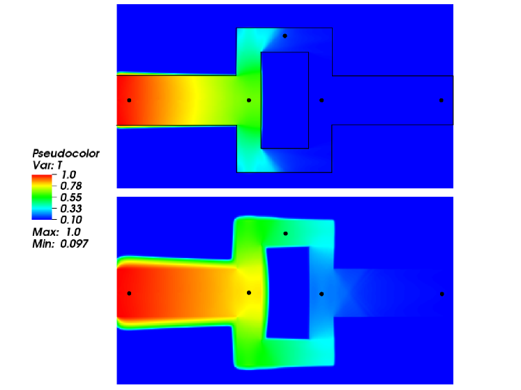
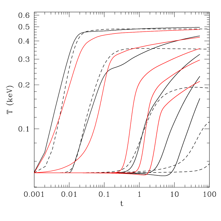
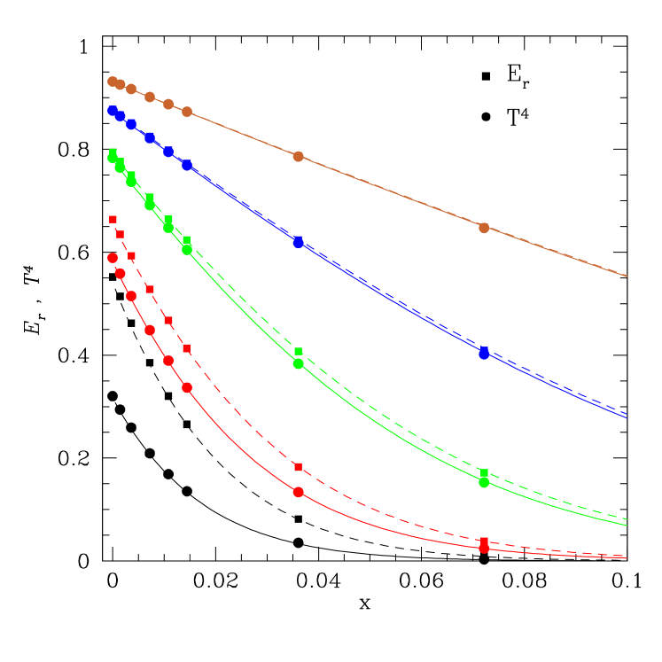
First, we fix the time step to be $4\times 10^{-5}$ to resolve the light crossing time. Snapshots of the temperature distribution at two different times are shown in Figure 4. Note that the shadows around the corners of the pipe are captured properly. Five probes are placed at $(x=0.25,y=0)$, $(x=2.75,y=0)$, $(x=3.5,y=1.25)$, $(x=4.25,y=0)$ and $(x=6.75,y=0)$ to monitor the change of the temperature in the pipe. The time evolution of the temperatures at the five points are shown as solid black lines in Figure 5. Compared with Figure 9 of Gentile (2001), which shows the result calculated with a Monte Carlo method, our first-order backward Euler method with VET gives very similar results when the time step is small enough to resolve the light crossing time. For the fifth point, note that it cools off slightly before being heated by the radiation wave, in agreement with the behavior noted by Gentile (2001). The most obvious difference in our solution compared to Gentile (2001) is that the temperature of the first two points increases too quickly. This is likely due to the fact that we neglect the light travel time in our short-characteristic module when we calculate the VET. Thus the first two points are affected by the heating source too early. We also find the evolution of the last three points to differ in detail from that shown by Gentile (2001), however for these points the difference between propagation in cylindrical versus planar (Cartesian) geometry may be important. In our solution, there is no geometrical dilution of the flux as it propagates radially, and therefore the heating rate per unit surface area on the walls of the pipe is increased. This can affect the detailed temporal evolution at the third through fifth probes. Most importantly, note that from Figure 4 our first order implicit update can maintain very sharp gradients in the temperature at the walls of the pipe.

As a second test of our method, we repeat the problem using a time step of $10^{-3}$ initially, and increasing it by a factor of $1.1$ at each step until it reaches $1$. The result is shown as the dashed line in Figure 5. With this larger time step, the error in the temporal evolution of the probes is increased, although the basic evolution is still correct. This is consistent with our expectations. If we are not interested following evolution on a light crossing or thermalization time, we can use a large time step and still maintain a stable solution with the correct asymptotic behavior. Instead, if we want to explore the evolution on these time scales, we must use a small enough time step to resolve them.

A second method to evolve the material temperature with our algorithms is to add the radiation energy source term based on the solution of the time-independent transfer equation used to calculate the VET. Details of how to compute the material heating rate from the solution of the transfer equation are given in Davis et al. (2012). We call this algorithm method II. The solution computed using this method for the tophat test is shown as red lines in Figure 5. The time step is fixed to be $10^{-3}$. The result does not change substantially when we decrease the time step further. This method also gets a very similar solution as that shown in Figure 9 of Gentile (2001). Once again, the material is heated up too quickly everywhere but the location of the first probe. Again, this is likely due to the fact that the short characteristic module solves the time-independent radiation transfer equation, so that we ignore the delay due to the finite speed of propagation of radiation down the pipe. The last three points also differ because of our use of a planar geometry. Nevertheless, method II still captures the basic evolution correctly.

Other stringent test of our radiation transport module used to calculate the VET (such as the beam test), are described in detail in Davis et al. (2012), and will not be repeated here.

6. Tests of the Full Algorithm

In SS10, tests of various aspects of the one dimensional version of the algorithm used here were presented, and we have verified that our extension to multidimensions is able to pass all of these same tests. However, more rigorous testing requires solutions to the full system of equations of radiation hydrodynamics in multidimensions. Unfortunately, unlike the case of hydrodynamics or MHD, there are very few such solutions available. In the following subsections, we describe the results of the suite of test problems we have found most useful.

6.1. Linear Wave Convergence

The dispersion relation for linear wave solutions to the radiation hydrodynamic equations in a uniform homogeneous background medium, and assuming the Eddington approximation (fixed Eddington factor ${\sf f}=1/3{\sf I}$), have been analyzed by a variety of authors (e.g., Mihalas & Mihalas, 1984; Bogdan et al., 1996; Johnson & Klein, 2010). These authors solve the boundary value problem in which a complex wave number $k$ is found for each real frequency $\omega$. Johnson & Klein (2010) have used these solutions to test the Lagrangian radiation hydrodynamic code KULL by driving the waves with a time-dependent boundary condition; similar tests were used earlier by Turner & Stone (2001) to test the flux-limited diffusion module in the ZEUS code.

In contrast, Lowrie et al. (1999) give the dispersion relation for linear waves (again in the Eddington approximation) as an initial value problem, that is solving for the imaginary frequency $\omega$ at fixed real $k$. Although their analysis focused on the properties of linear waves in a moving fluid (they point out that in radiation hydrodynamics, linear wave solutions are not Galilean invariant), their approach is ideally suited for code tests. It allows the propagation of linear waves to be followed in a periodic domain, free from the complexity of the implementation of driving boundary conditions in an Eulerian code, which may in and of itself introduce spurious error into the solutions. The dispersion relation for linear waves in radiation MHD has also been considered by Blaes & Socrates (2001) and Blaes & Socrates (2003). We use both the hydrodynamic and MHD linear wave solutions for convergence testing in $1D$, $2D$, and $3D$ in the following subsections. We emphasize that in order to keep the solutions to the dispersion relation analytic so that they can be used in the test problems, the Eddington approximation must be adopted. There may be regions of parameter space where the Eddington approximation is not appropriate, and the properties of linear waves in this regime should be computed using a variable Eddington factor computed self-consistently with flow. However such solutions are beyond the scope of this paper.

It is not possible to simply initialize this test problem using previous solutions for linear waves given in the literature, because there may be differences in the frame of reference, and in the order of the source terms kept, in the fundamental system of dynamical equations (our equation 1). For this reason, we have rederived the dispersion relation for linear waves in the system of equations solved by our code. Even with the Eddington approximation, these solutions are non-trivial, requiring finding the roots of a fourth-order polynomial for complex $k$ in hydrodynamics, and a tenth-order polynomial for $k$ in MHD. Appendices B and C give the details of our solutions in the case of hydrodynamics and MHD respectively, while in Tables 1 through 3 we give the complete eigenvector for linear waves for several parameter values for use by others.

6.1.1 Linear Waves in Radiation Hydrodynamics

We begin by studying the propagation of linear waves in one dimension with hydrodynamics. We consider a uniform, homogeneous medium with background state $\rho=T=P=1$, adiabatic index $\gamma=5/3$, and zero velocity initially. The radiation flux is zero, and the radiation energy density $E_{r}=1$ initially for all of the calculations. We assume a constant absorption opacity $\sigma_{a}$ (perturbations of the opacity will always be second order, which can be neglected), and zero scattering opacity. In order to adopt the Eddington approximation, we fix the Eddington tensor to be diagonal with components $f_{ii}=1/3$. The dimensionless speed of light ${\mathbb{C}}=10^{4}$. We use a domain of size $L=1$ with 512 grid zones, and periodic boundary conditions for all variables at each edge. We initialize a wave solution (Appendix B) by adding an eigenmode (see Table 1) with a wavelength equal to the size of the domain $L$, and an amplitude of $10^{-6}$.

We perform a series of calculations in which we study the effect of varying the radiation to gas pressure ratio by varying the dimensionless pressure ${\mathbb{P}}$, while keeping the initial conditions fixed as above. We also study the effect of varying the optical depth per wavelength $\tau_{a}=\sigma_{a}L$ by varying the absorption opacity $\sigma_{a}$. For each of these calculations, we measure the phase velocity of the waves by determining how long it takes a fixed feature in the wave (the density maximum) to propagate a distance equal to one wavelength ($L=1$). We also measure the damping rate of the wave by determining the best fit amplitude to the entire wave profile after one period. We then compare these results to linear theory.

The properties of radiation modified linear acoustic waves vary dramatically with optical depth and pressure ratio. Two dimensionless numbers can be used to define various regimes. The first, ${\mathbb{P}}{\mathbb{C}}\tau_{a}$, measure the importance of energy exchange between the radiation field and the material, while the second, ${\mathbb{P}}\tau_{a}$, measures the importance of momentum exchange. When both ${\mathbb{P}}{\mathbb{C}}\tau_{a}\ll 1$ and ${\mathbb{P}}\tau_{a}\ll 1$, energy exchange between the radiation field and material is very weak, the momentum of the radiation field can be neglected, so the waves are weakly damped and propagate at nearly the adiabatic sound speed. The damping rate increases with optical depth until $\tau_{a}\sim 1$; thereafter the radiation and material energy densities are strongly coupled, and the damping rate decreases with increasing optical depth. When ${\mathbb{P}}{\mathbb{C}}\tau_{a}\gg 1$ and ${\mathbb{P}}<1$, the radiation and material energy densities are strongly coupled but the radiation momentum is still negligible, therefore in this case the damping rate decreases with optical depth until $\tau_{a}\sim 1$, and increases thereafter. Finally, if ${\mathbb{P}}{\mathbb{C}}\tau_{a}\gg 1$ and ${\mathbb{P}}>1$, the momentum in the photons becomes important, and the damping rate reaches a minimum when ${\mathbb{P}}\tau_{a}\sim 1$ and increase afterwards. To ensure our algorithms are accurate over a wide range of regimes, it is important to perform tests that span these dimensionless parameter values. These dimensionless quantities also clarify a potential shortcoming with numerical algorithm based on the reduced speed of light approximation (e.g., Gnedin & Abel, 2001). Any arbitrary reduction in the speed of light will reduce ${\mathbb{C}}$ and the above dimensionless numbers correspondingly, which will alter the damping rate and phase velocity of the radiation modified acoustic wave.

In addition to ${\mathbb{P}}$ and ${\mathbb{C}}$, the Boltzmann number Bo is another dimensionless number which is useful to quantify the relative importance of radiative and material energy transport in a radiating flow (e.g., Mihalas & Mihalas, 1984); it is defined to be the ratio between the material enthalpy flux and radiative flux from a free surface. It is related to our dimensionless numbers ${\mathbb{P}}$ and ${\mathbb{C}}$ as

$$\text{Bo}=\frac{4\tilde{v}\gamma}{\mathbb{PC}(\gamma-1)},$$ (41)

where $\tilde{v}\equiv v/a_{0}$, is the typical flow velocity in units of $a_{0}$. In the linear wave tests, the typical flow velocity $v$ can be replaced with the adiabatic sound speed. When Bo is small, energy transport is dominated by radiation field and material energy transport is dominant when Bo is large.

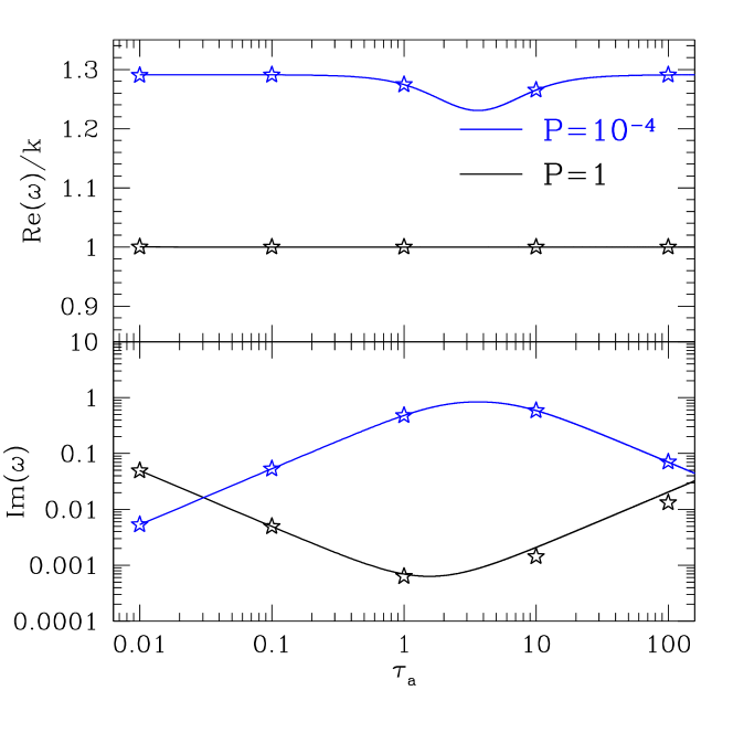
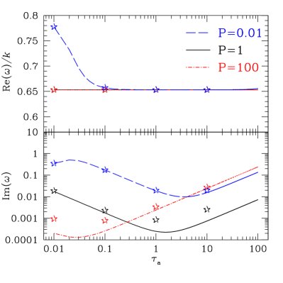
Figure 6 compares the numerically measured phase velocity and damping rate (shown as stars) for two different radiation pressures, and over a wide range of optical depths $\tau_{a}$, in comparison to the solution of the linear dispersion relation (equation B1) shown as solid lines. The parameters are chosen such that for the runs with ${\mathbb{P}}=10^{-4}$, the dimensionless number ${\mathbb{P}}{\mathbb{C}}\tau_{a}$ spans $10^{-2}\leq{\mathbb{P}}{\mathbb{C}}\tau_{a}\leq 10^{2}$, while for the runs with ${\mathbb{P}}=1$ both of these limits are a factor of $10^{4}$ larger. Based on the discussion above, for ${\mathbb{P}}=10^{-4}$ we expect the damping rate to increase until $\tau_{a}\sim 1$ and decrease thereafter, while for ${\mathbb{P}}=1$ we expect the opposite. The solid lines from the analytic solution of the dispersion relation clearly show these trends. In addition, the numerically measured phase velocity agrees with the analytic results over the entire range of optical depths for both values of the radiation pressure, while the damping rate is accurate in all cases except when ${\mathbb{P}}=1$ and $\tau_{a}\geq 1$. However, for these parameter values, the damping rate is small and the numerical measured damping rates are not converged at the resolution used for this plot. We have confirmed that if we increase the resolution, the numerical measured damping rate converges to the analytic values. At the same time, we have also found when $\tau_{a}\geq 100$, our algorithm no longer reproduces the correct damping rate. We discuss this further, and suggest a solution, below. When ${\mathbb{P}}=10^{-4}$, Boltzmann number $\text{Bo}=10$ and it is $10^{-3}$ when ${\mathbb{P}}=1$. In the case ${\mathbb{P}}=100$, Bo is only to $10^{-5}$.

Figure 6.— Phase velocity scaled to the isothermal sound speed (top panel) and damping rate (lower panel) of linear acoustic waves versus the optical depth per wavelength for two different radiation pressures. The stars represent quantaties measured from simulations, while the lines come from the solution to the linear dispersion relation (equation B1). All simulations are performed in 1D with 512 grid points per wavelength.

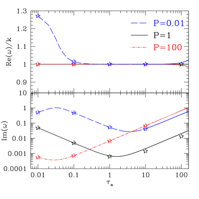
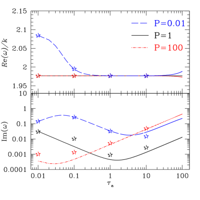
In Figure 7 we test linear wave propagation over a wide range of radiation pressures. Once again, the left panel compares the numerically measured phase velocity and damping rate (shown as stars) for three different radiation pressures, and over a wide range of optical depths $\tau_{a}$, in comparison to the solution of the linear dispersion relation (equation B1) shown as solid lines. Even though the properties of radiation modified linear acoustic waves vary dramatically over this range of optical depths and pressure ratios, there is good agreement between the numerical and analytic solutions, except when ${\mathbb{P}}=1$ and $\tau_{a}>1$. For these parameters, we also find at higher resolution, our algorithm converges to the analytic damping rate, suggesting that the discrepancy is dominated by numerical diffusion at this resolution.

Figure 7.— Left. Phase velocity scaled to the isothermal sound speed (top panel) and damping rate (lower panel) of linear acoustic waves versus the optical depth per wavelength for three different radiation pressures. The stars represent quantities measured from simulations, while the lines come from the solution to the linear dispersion relation (appendix B). All simulations are performed in 1D with 512 grid points per wavelength. Numerically measured values of both quantaties agrees with linear theory when the absorption optical depth per wavelength is smaller than $\sim 100$. Right. Convergence of L1 error with resolution for two different sets of parameters. Both simulations are in full 3D. The radiation dominated case converges at first order, while the gas pressure dominated case converges at second order as expected (see text).

Note that in Figure 7 we do not plot the numerical solution for $\tau=100$ and ${\mathbb{P}}=100$ or $0.01$. We have found the damping rate of linear waves stops converging for these parameter values. Our tests reveal that the problem is associated with our implicit solution of the radiation subsystem at a timestep determined by the adiabatic sound speed in the material. In this regime, an accurate solution require a timestep which resolves the light crossing time across a cell. Note we find this is only an issue for very large absorption opacity: large scattering opacities do not couple the radiation and material energy densities. When the optical depth per wavelength due to the absorption opacity becomes so large (${\mathbb{P}}\tau_{a}\sim{\mathbb{C}}$) that the radiation field and the material can be treated like a single fluid, we have found it is more accurate to solve a single system of conservations laws for the total (radiation plus material) energy and momentum, rather than splitting the radiation subsystem from the material conservation laws.

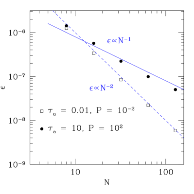
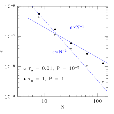
As our next test, we measure the convergence rate of linear waves in 3D, for two different values of the problem parameters. We use a computational domain of size $2L\times L\times L$, with the same number of grid cells per unit length $L$ in each direction. We initialize the one dimensional solution inclined to the grid using the same technique to compute the appropriate volume averages of the solution as described in (Stone et al., 2008). We propagate the wave for one period, and then measure the L1 error in the solution from

$$\delta{\bf q}=\frac{1}{N}\sum_{i}|{\bf q}_{i}-{\bf q}_{i}^{0}|$$ (42)

where ${\bf q}_{i}^{0}$ is the initial solution, and the sum is taken over all grid points. We repeat this calculation for a variety of different numerical resolutions (grid cells per unit length $L$), and plot the change in the L1 error with resolution. The result is shown in the right panel of Figure 7 for a radiation dominated, optically thick fluid (${\mathbb{P}}=10^{2}$, $\tau_{a}=10$), denoted by the solid circles, and for a gas pressure dominated, optically thin fluid (${\mathbb{P}}=10^{-2}$, $\tau_{a}=10^{-2}$), denoted by the open squares. In the radiation dominated case the errors converge close to first order, while in the gas pressure dominated case, the errors converge close to second order. This behavior is expected. The errors in the former are dominated by the solution to the radiation subsystem, which uses a first-order accurate backward Euler step for stability. Thus, we expect the overall rate of convergence should be first order. On the other hand, in the gas pressure dominated case, the errors are dominated by the solution to the material conservation laws, which uses a second-order accurate modified Godunov step. In this case, the overall rate of convergence should be second order. Of course, it might be possible to increase the rate of convergence in the implicit solution of the radiation moment equations by adopting higher order implicit differencing. However, limiting such methods to enforce monotonicity can be problematic (e.g., SS10). We prefer to adopt unconditionally stable first-order methods for the implicit solver.

Linear wave solutions when only radiation energy source terms are added with radiation momentum source terms neglected are also given by Davis et al. (2012) and used to test our radiation transfer module (see Figure 9 of that paper). Because the radiation energy source term is added explicitly, the radiation diffusion mode needs to be resolved to make the code stable, which can limit the time step significantly when $\text{Bo}\lesssim 1$. Therefore the algorithm of Davis et al. (2012) is most suitable for the regime $\text{Bo}>0.01$. Because we include all the radiation momentum and energy source terms, the dispersion relations given in this paper differ from Figure 8 of Davis et al. (2012). However, in regimes of parameter spaces which overlap, we do get very similar results, for example when ${\mathbb{P}}=10^{-4}$ and $\text{Bo}=10$ shown in Figure 6.

6.1.2 Linear Waves in radiation MHD

Next, in order to test the accuracy of our MHD algorithms with radiation, we consider the propagation of linear modes of radiation modified magnetosonic waves. We do not consider Alfvén waves in this subsection since they are incompressible and are affected less by radiation than magnetosonic modes. In the case of radiation modified MHD waves, the transverse components of the velocity must be included even for 1D solutions. However, as implemented our code does not include the transverse velocities in 1D during the implicit solution of the radiation moment equations. Thus, all of the MHD tests presented here have been performed in 2D using a grid of either $512\times 64$, or in some cases $1024\times 64$ cells.

For these MHD tests, we use a uniform, homogeneous medium with the hydrodynamic and radiation variables set to the identical values as were used for the hydrodynamic test (see the previous subsection). The strength of the magnetic field is $B_{0}=\sqrt{5/3}$ (which gives a ratio of the Alfvén to sound speed of 2). The direction of the magnetic field is 45 degrees to the $x-$axis, and it is confined to the $x-y$ plane (so $B_{z}=0$). We use a 2D domain of size $L\times L$ with $L=1$ with periodic boundary conditions for all variables at each edge. As before, we initialize a wave solution (Appendix C) by adding an eigenmode (see Tables 2 or 3) propagating in the $x-$ direction with a wavelength equal to then size of the domain $L$, and an amplitude of $10^{-6}$. Once again, we perform a series of calculations in which we study the effect of varying the radiation to gas pressure ratio by varying the dimensionless pressure ${\mathbb{P}}$, and the effect of varying the optical depth per wavelength $\tau_{a}=\sigma_{a}L$ by varying the absorption opacity $\sigma_{a}$.

The results of our tests for slow magnetosonic waves are shown in Figure 8, while the results for fast magnetosonic wave are shown in Figure 9. The left panel in each figure compares the numerically measured values of the phase velocity and damping rate with linear theory. Note that the solution to the dispersion relation as a function of optical depth and ${\mathbb{P}}$ for both magnetosonic modes is very similar to that for radiation modified acoustic waves in hydrodynamics (see Figure 9). Once again, we find good agreement between our numerical values for the phase velocity versus linear theory over this parameter regime. The damping rate also shows good agreement, except when ${\mathbb{P}}=100,\tau_{a}<1$ and ${\mathbb{P}}=1,\tau_{a}>0.1$. In these cases, the damping rate is so small that our numerical measured values are not converged at this resolution. Nevertheless, as Figure 9 demonstrates, our algorithm converges to the correct solution for ${\mathbb{P}}=1,\tau_{a}=1$, albeit at first order. We have confirmed our algorithm also converges for the other parameters shown in this figure as well.

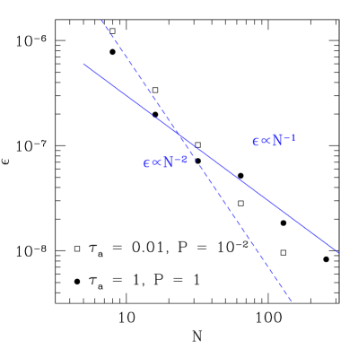
The right panels of Figures 8 and 9 show the convergence rate of the L1 error with numerical resolution for the slow and fast magnetosonic waves respectively in a fully 3D domain of size $2L\times L\times L$. As before, we measure first-order convergence in a parameter regime where the solution to the radiation moment equations dominates the error, and second-order convergence in the opposite limit.

Figure 8.— Phase velocity scaled to the isothermal sound speed (top panel) and damping rate (lower panel) of linear slow magnetosonic waves versus the optical depth per wavelength for three different radiation pressures. The stars represent quantaties measured from simulations, while the lines come from the solution to the linear dispersion relation (appendix C). All simulations use an effective resolutions of 512 grid points per wavelength (except for the two runs with $P=100$ and $\tau_{a}<1$, which use 1024 grid points per wavelength). Numerically measured values of both quantaties agree with linear theory over the entire range of parameter space, except for very low damping rates, where numerical diffusion dominates. Right. Convergence of L1 error with resolution for two different sets of parameters. Both simulations are in full 3D. The radiation dominated case converges at first order, while the gas pressure dominated case converges at second order, as in the case of hydrodynmaics.

Figure 9.— Same as figure 8, but for fast magnetosonic waves.

6.2. Radiative shocks in the non-equilibrium diffusion limit

Shock tubes have long been used as a test of hydrodynamic and MHD codes in the nonlinear regime, since the structure of a planar shock can be computed analytically in these cases. However, in radiation hydrodynamics and MHD, shock structure is much more complicated, and is difficult to compute analytically. At low Mach numbers $\mathcal{M}$, radiation can diffuse upstream of the shock, heating the gas and forming a smooth precursor in the temperature. As $\mathcal{M}$ increases, the gas temperature near the shock front can begin to exceed the downstream value, forming a Zel’dovich spike (e.g., Zel’Dovich & Raizer, 1967; Mihalas & Mihalas, 1984). This spike is followed by a relaxation region where the gas temperature cools to its far downstream value. When a Zel’dovich spike is formed, if the downstream gas temperature (after the relaxation region) is larger than the value immediately upstream of the shock (at the end of the precursor region), the shock is called subcritical. On the other hand, if the downstream gas temperature after the relaxation region is the same as the upstream gas temperature, the shock is termed supercritical. Subcritical shocks are formed at lower $\mathcal{M}$ than supercritical shocks. Finally, as $\mathcal{M}$ is increased further, the downstream radiation pressure can exceed the gas pressure, the Zel’dovich spike disappears, and the solution becomes everywhere smooth again.

Although many authors have presented numerical solutions to radiating shocks as a test of their algorithms, the lack of analytic solutions inhibits quantitive testing. Recently Lowrie & Edwards (2008) have studied the structure of radiation modified shocks in the non-equilibrium diffusion limit as a function of Mach number. They give a very clear explanation of how these structures can be computed by combining smooth solutions to ordinary differential equations with discontinuous jumps determined by the Rankine-Hugoniot relations when needed. These solutions not only provide interesting insight into the structure of radiating shocks, but also provide an quantative test of time-dependent radiation hydrodynamic codes.

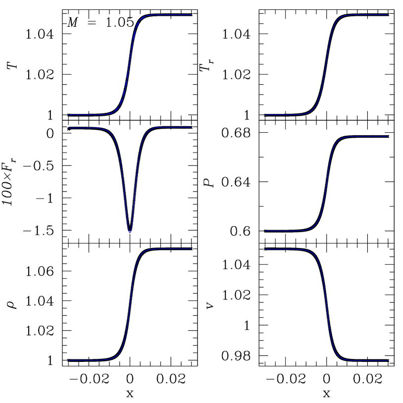
To test our algorithms, we follow the semi-analytic method described in Lowrie & Edwards (2008) (hereafter LE) to calculate the shock structure at a variety of Mach numbers, using a non-dimensional pre-shock solution of $\rho_{0}=T_{0}=E_{r,0}=1$ and $v_{0}=\mathcal{M}$ in the upstream state. We then initialize this solution on a 1D grid by volume averaging each conserved variable to our numerical mesh. The LE solutions are given in the co-moving frame, thus we transform the co-moving radiation flux and energy density to the Eulerian frame, using equation 7. In order to make our solutions match those presented in LE, we use a dimensionless speed of light ${\mathbb{C}}=1.732\times 10^{3}$ and pressure ${\mathbb{P}}=10^{-4}$ and absorption and scattering opacities of $\sigma_{a}=\sigma_{t}=577.4$. The gas temperature $T$ is calculated as $T=P/(0.6\rho)$ and $\gamma=5/3$. The Eddington approximation is used so $P_{r}=E_{r}/3$. We use a computational domain of size $L$, where $L$ is large enough to capture the upstream precursor and downstream radiative relaxation regions (the size of these regions are given by the LE solution itself), with a grid of $1024$ cells in all cases (except $\mathcal{M}=50$ where we we use $2048$ cells). Input boundary conditions at the upstream values are used on the left, and outflow boundary conditions are used on the right, with the shock propagating in the negative $x$-direction. We then let the code evolve this solution for several flow crossing times, $t_{f}=L/\mathcal{M}$. Ideally, the solution should remain stationary on the mesh. A small shift in the position of the shock front can be expected due to truncation error in the averaging of the initial solution to the hydrodynamic grid. A serious error in the algorithm or its implementation would be revealed if the code cannot hold the input solution.

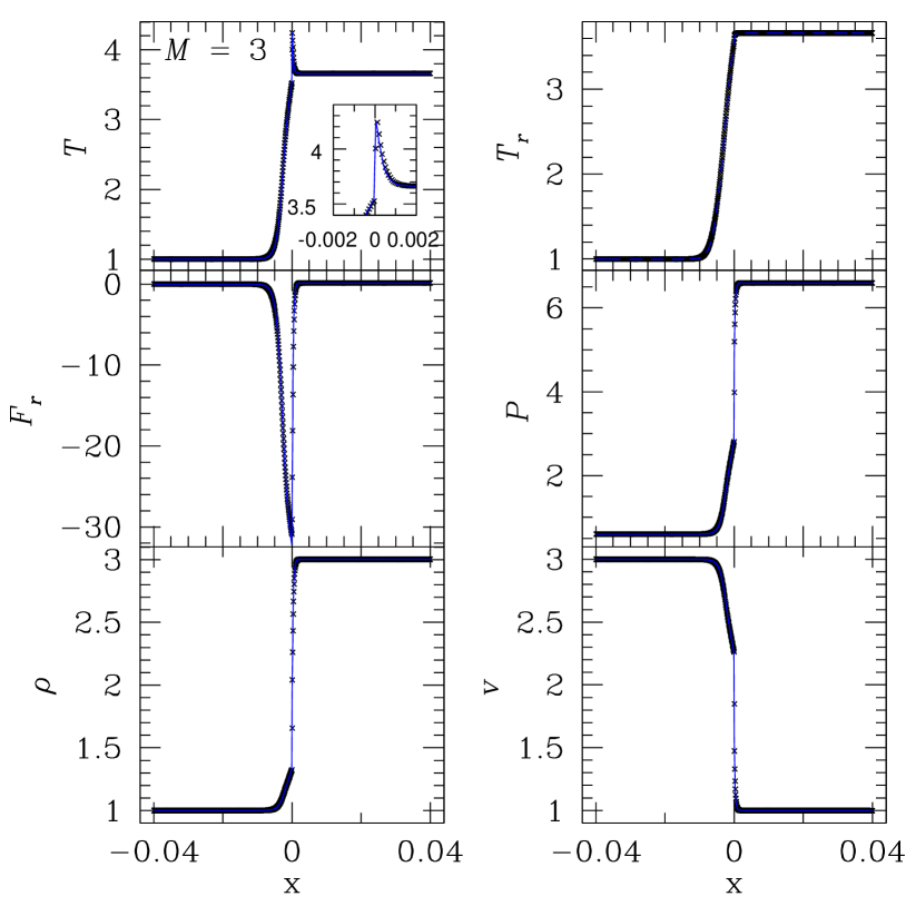
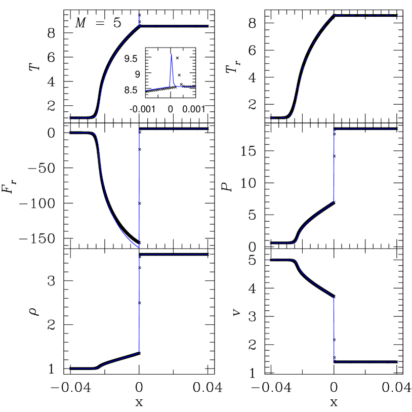
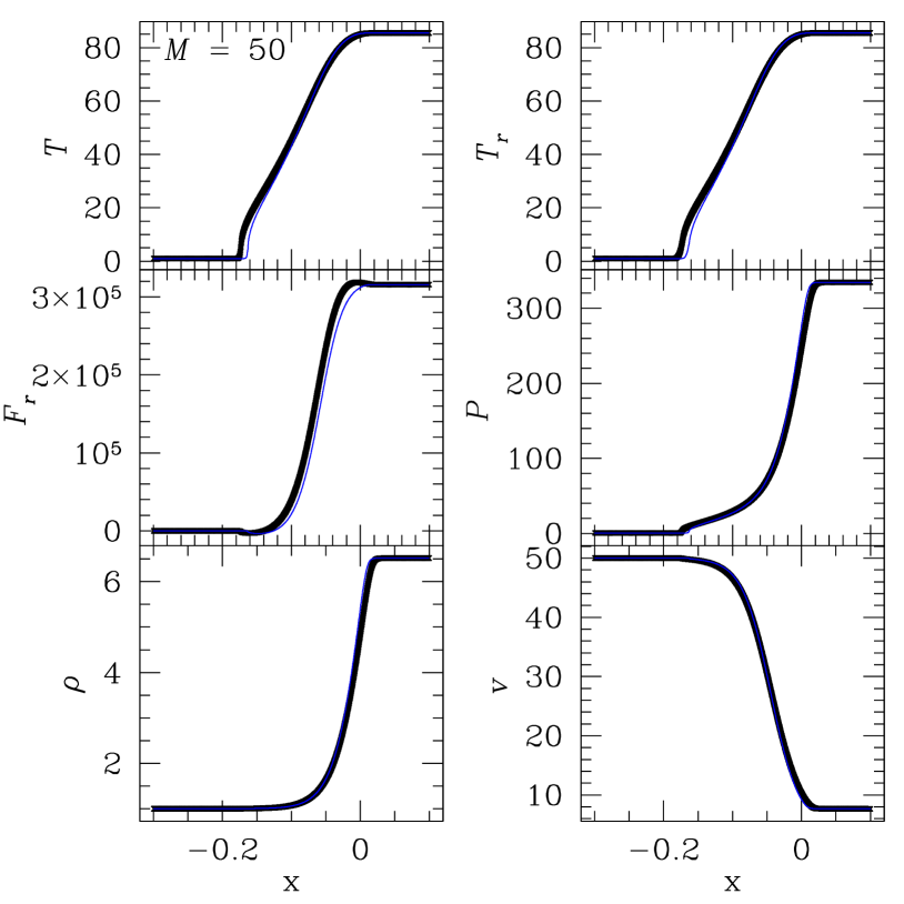
We begin by presenting our numerical solution for $\mathcal{M}=1.05$ in Figure 10. In this case there is no discontinuous jump in any variable, but rather only a smooth precursor. Next, Figure 11 shows the solution for $\mathcal{M}=3$. Now a discontinous shock jump has appeared, along with a Zel’dovich spike. For these parameters, this shock is subcritical. The inset panel in the plot of gas temperature shows a blow-up of the region near the spike. The numerical solution shows agreement with the semi-analytic solution of LE. Next, Figure 12 shows the solution for $\mathcal{M}=5$. Now there is a discontinuous jump in some variables (such as density and velocity), but the gas temperature is continuous apart from the Zel’dovich spike. This solution corresponds to a supercritical shock. Again, the blow-up of the gas temperature near the spike region reveals agreement between the numerical and semi-analytic solutions. The position of the spike has moved a few cell widths, but has quickly relaxed to a steady structure at the correct shock speed. Finally, Figure 13 shows the solution for $\mathcal{M}=50$. In this case, the radiation pressure is about $10$ times gas pressure in the downstream flow. Now all variables are smooth, with no jumps.

Figure 10.— Strucure of a radiation modified shock for Mach number $\mathcal{M}=1.05$. Blue lines are initial conditions, while black dots are numerical results after a few flow crossing times.

Figure 11.— Same as figure 10, but for $\mathcal{M}=3$. At this Mach number, a subcritical shock is formed. Inset in the gas temperature panel shows details of the Zel’dovich spike.

Figure 12.— Same as figure 10, but for $\mathcal{M}=5$. At this Mach number, a supercritical shock is formed. Inset in the gas temperature panel shows details of the Zel’dovich spike.

Figure 13.— Same as figure 10, but for $\mathcal{M}=50$. At this Mach number, the downstream flow is radiation pressure dominated.

LE have shown that the gas temperature profile near the shock front is very sensitive to small changes in $\mathcal{M}$ when $\mathcal{M}$ is small. To explore whether our algorithms can capture these subtle changes, Figure 14 plots the gas temperature for six Mach numbers between $\mathcal{M}=1.05$ and 5. The values are chosen to correspond to figures 4 through 11 of LE, where these changes are noted and discussed. This region covers the formation of a Zel’dovich spike, and the increase in the amplitude of the spike with increasing $\mathcal{M}$. It is clear from the figure, in which the numerical solution is compared to the corresponding solution from LE, that our algorithm captures each phase accurately.

Figure 14.— Gas temperature profiles with different Mach number for radiation modified shocks. Blue lines are the initial conditions, while black dots are the numerical solution after a few flow crossing times. Note the subtle changes in the shock structure between $\mathcal{M}=1$ and 2, which are clearly captured in the numerical solutions.

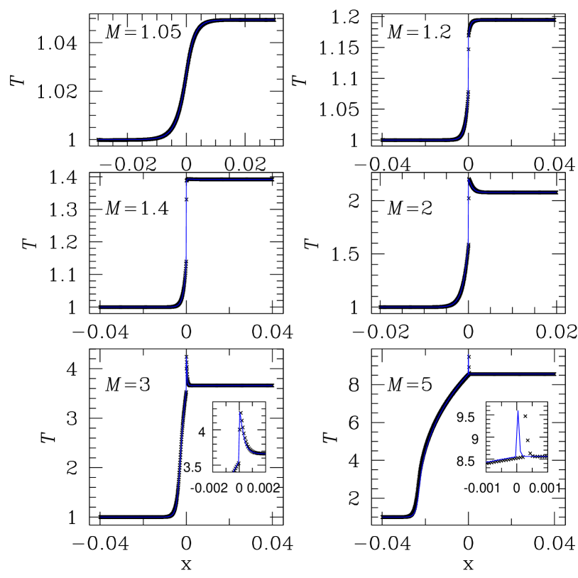
Figure 14 shows that our algorithm captures the transition from subcritical to supercritical shocks accurately at low $\mathcal{M}$, while figure 13 shows the solution with $\mathcal{M}=50$ (in the stongly radiation pressure dominated regime) is also captured accurately. However, we have found solutions at $\mathcal{M}\approx 30$ are inaccurate at the resolutions we use. As the Mach number increases beyond $\mathcal{M}=5$, the width if the Zel’dovich spike compared to the width of the precursor region gets smaller, until the spike disappears in the radiation pressure dominated case near $\mathcal{M}=50$. We find that unless the grid resolution is smaller than the thickness of the Zel’dovich spike, our algorithm will not hold a steady solution. For example, at $\mathcal{M}=30$ this would require a resolution of about $10^{6}$ cells for a uniform grid. Clearly, in this case either static or adaptive mesh refinement would be useful to resolve the spike. With enough resolution to resolve the spike, our algorithms provide an accurate solution in this regime.

6.3. Radiative shocks with a variable Eddington tensor

Calculating the structure of radiation modified shocks without invoking the Eddington approximation or other simplifying assumptions is extremely challenging. Sincell et al. (1999) have used a time dependent radiation hydrodynamics code to compute the structure of radiation modified shocks. We have found that comparison of our solutions in this regime to the results reported by Sincell et al. (1999) is a useful code test.

In many ways, the numerical algorithm used by Sincell et al. (1999) is similar to that described here. They solve the radiation moment equations using a variable Eddington factor computed from a formal solution of the transfer equation, assuming LTE and gray opacities. However, the underlying hydrodynamic solver they use is quite different from that adopted in this work. Sincell et al. (1999) use methods based on artificial viscosity for shock capturing, and solve the internal rather than total gas energy equation. The Godunov methods used here use Riemann solvers rather than artificial viscosity for shock capturing, and are based on the total gas energy equation.

Since the Mach number $\mathcal{M}$ is not known independently of the shock structure, it is not possible to compute the solution in the frame of the shock. Instead, we initialize a flow that generates a shock, and allow the shock to propagate a large enough distance to settle into a steady structure. To generate the shock, we collide two symmetric flows at the center of the domain, producing two identical shocks that propagate symmetrically away from the center. This avoids having to implement reflecting boundary conditions in the radiative transfer solver that is used to compute the VET (Davis et al., 2012) necessary if the shock is generated by reflection of the flow off a wall. The initial conditions for the flow are chosen to match those used by Sincell et al. (1999) (see also SS10) for the subcritical shock solution discussed in §2.1 of their paper. We use a computational domain that spans $-2\leq x\leq 2$. Initially, the density is one, the gas pressure is $P=0.923\rho T$, and the gas temperature is $T=1+7.5|x|/2$. For $x<0$, the flow velocity is $v=20$, while for $x>0$ it is $v=-20$. The dimensionless pressure and speed of light are ${\mathbb{P}}=1.08\times 10^{-10}$ and ${\mathbb{C}}=10^{6}$, and $\gamma=5/3$. The radiation temperature is the same as gas temperature, the radiation flux is ${\mbox{\boldmath$F$}}_{r}=-(\partial E_{r}/\partial x)/(3\sigma_{a})$ (the Eddington approximation is assumed in the initial condition only because the density is uniform initially), where the absorption opacity $\sigma_{a}=10$. The VET is initialized with only non-zero diagonal components of $1/3$; thereafter the VET is computed self-consistently with the flow using short characteristics.

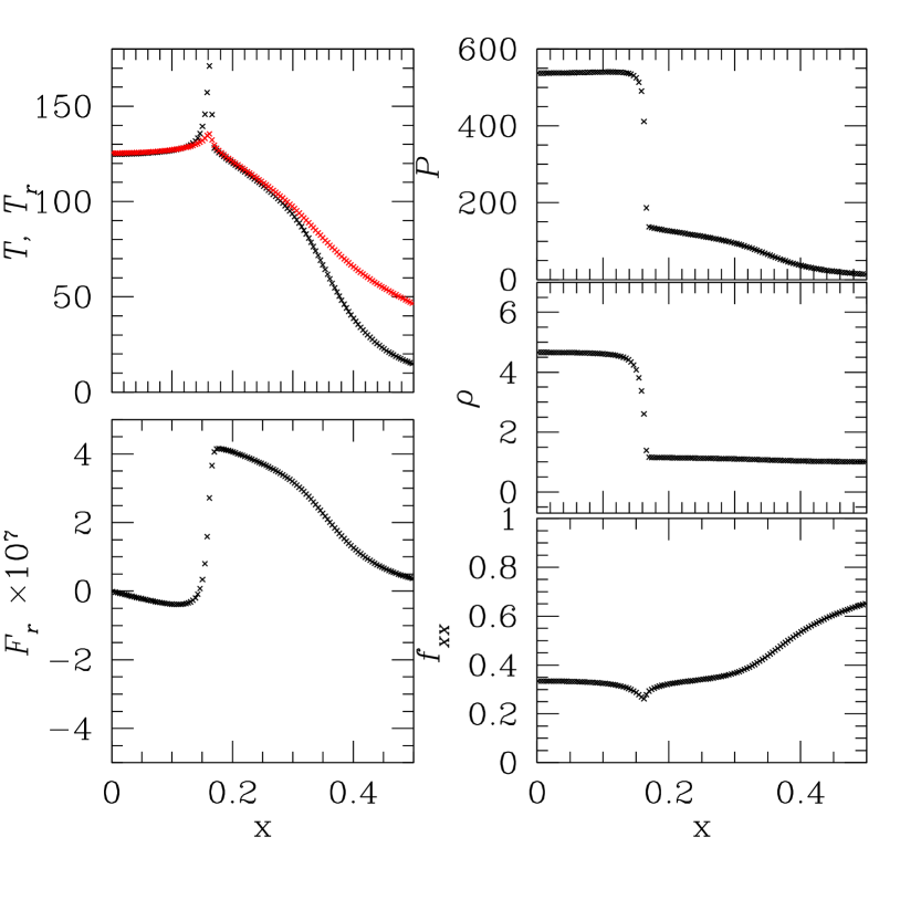
Profiles of various quantities at $t=0.03$ are shown in Figure 15 in the region $0\leq x\leq 0.5$. (We have checked, as another test of our code, that the solution is exactly symmetric with respect to $x=0$.) Profiles of each variable show the characteristic structure of a subcritical shock, including a strong radiative precursor and Zel’dovich spike. Perhaps of greatest interest is the profile of the $x-x$ component of the VET shown in the lower right panel. Upstream of the shock $f_{xx}$ is much bigger than 1/3, as expected. Downstream of the shock, it is close to $1/3$. However, in the vicinity of the shock itself, $f_{xx}$ is smaller than $1/3$, in agreement with the results of Sincell et al. (1999) (see their figure 8). The reason for the behavior is discussed in §2.3 of Sincell et al. (1999). Most of the upstream radiation is generated within one optical depth of the shock front. Rays parallel to the shock front go through a longer path of source than rays perpendicular to the shock front. Thus, the intensity along rays parallel to the shock front is larger than those perpendicular, leading to a value of $f_{xx}$ less than $1/3$. Note that since the empirical relations for most flux limiters (e.g., Levermore & Pomraning, 1981) bound the Eddington factor between $1/3$ and one along the direction of radiation energy density gradient, FLD cannot get the right answer in this case.

Figure 15.— Structure of a subcritical shock computed with a VET at time $t=0.03$ in one dimension with $1024$ cells. In the upper left panel, the red line is the radiation temperature $T_{r}$ while the black line is the gas temperature $T$. Note that $x-x$ component of the Eddington tensor (lower right panel) can be smaller than $1/3$ near the shock front.

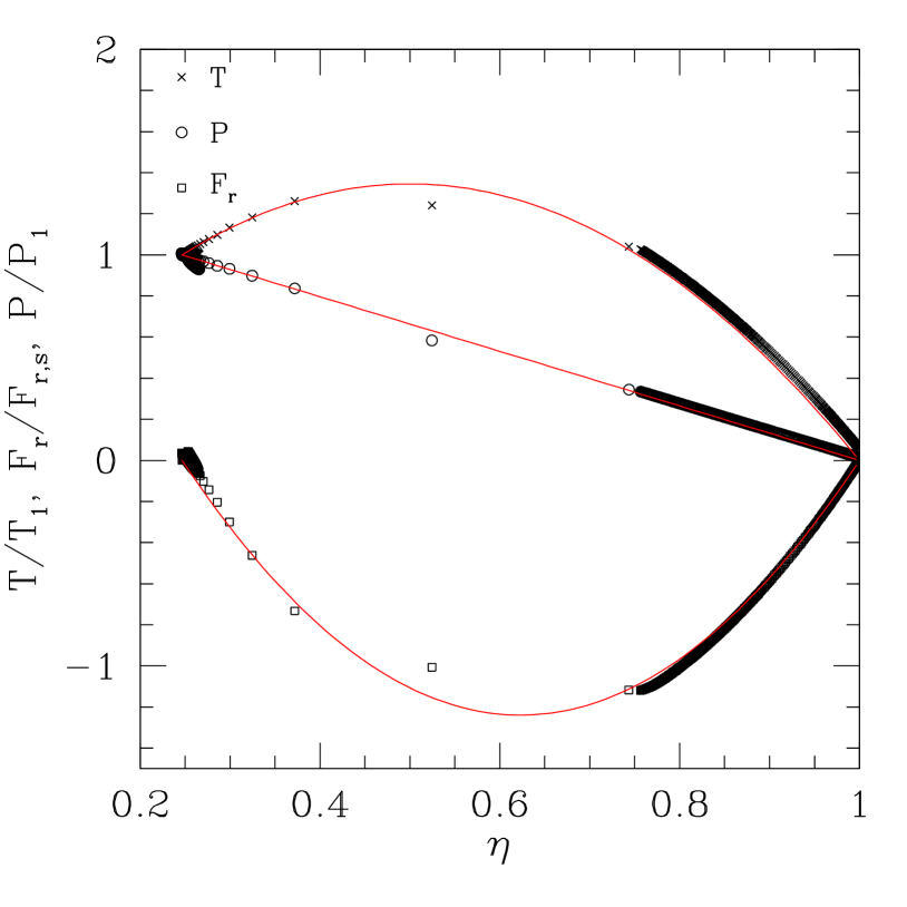
We find the most quantitative comparison to the previously published results of Sincell et al. (1999) is to plot the gas temperature, pressure, and radiative flux against the inverse compression ratio $\eta\equiv\rho_{0}/\rho$, where $\rho_{0}$ is upstream density. Figure 16 shows our result at $t=0.3$, for direct comparison to figures 2 and 3 in Sincell et al. (1999). An approximate analytic expression for these quantities by Zel’Dovich & Raizer (1967) (and also given in §1.3 of Sincell et al. (1999)) is shown as solid lines. The numerical solution of Sincell et al. (1999) is in fact in poor agreement with the analytic predictions, and these authors argue this is due to approximations made in the latter. It is clear from Figure 16 that our solutions agree very well with the approximate analytic solution, and therefore do not agree with the results of Sincell et al. (1999) for these quantities. Recall these authors use a numerical method based on artificial viscosity for shock capturing, and the internal rather than total energy equation. The plot measures the internal structure of the shock, which could be quite sensitive to both the form of viscosity used, and the degree to which energy is conserved. Our solution may be in better agreement with the analytic expectations since our algorithm uses a Riemann solver rather than artificial viscosity to capture shocks, and is based on the total energy equation.

Figure 16.— Gas temperature, radiation flux, and gas pressure as a function of inverse compression ratio $\eta\equiv\rho_{0}/\rho$, where $\rho_{0}$ is upstream density, for the subcritical radiative shock shown in Figure 15 at time $0.3$. Temperature and pressure are scaled by the downstream temperature $T_{1}$ and pressure $P_{1}$ at $x=0$, while the radiative flux is scaled by the flux $F_{r,s}$ at the shock front. Note $F_{r}$ is the co-moving flux. The red lines are analytic solutions given by Zel’Dovich & Raizer (1967) (see also Sincell et al. 1999).

6.4. Photon Bubble Instability

Photon bubble instability is an overstable mode present in radiation supported, magnetized atmospheres. It was first noticed in numerical simulations of neutron star polar cap accretion flows (Klein & Arons, 1989), and was subsequently confirmed in a linear stability analysis for neutron star atmospheres (Arons, 1992). More recently, Gammie (1998) and Blaes & Socrates (2003) recognized a similar instability occurs in accretion disk atmospheres, and analyzed the properties in the linear regime. Numerical simulations that investigate the non-linear regime were performed by Turner et al. (2005) using the FLD module in the ZEUS code (Turner & Stone, 2001). Since both the linear and non-linear regimes of this instability have been studied in detail in the literature, and since fundamentally it relies on radiation modified MHD waves, it provides is an excellent test of our radiation MHD algorithms in multidimensions. In this section, we repeat one set of parameters reported by Turner et al. (2005) and compare our results with solutions from ZEUS. In order to make direct the comparisons, we adopt the Eddington approximation, so that the diagonal components of the VET are fixed to be $1/3$.

The initial conditions consist of a stratified atmosphere in mechanical and thermal equilibrium, in which a uniform radiation flux balances gravity. The structure of the atmosphere is computed from the solution of the hydrostatic equilibrium equations

$$\frac{dP}{dy} = -\rho g+\sigma F_{r},\ \ P=\rho T,$$

$$\frac{1}{3}\frac{dE_{r}}{dy} = -\sigma F_{r},\ \ E_{r}=T^{4}.$$ (43)

with a constant gravitational acceleration $g=1$ in the $-\hat{y}$ direction, and an opacity of $\sigma=137.11\rho+0.15\rho^{2}T^{-3.5}$ (which includes both electron scattering opacity and Kramer’s opacity). The co-moving vertical radiation flux $\hat{F}_{r,0}=2.52\times 10^{-4}$. These equations are integrated in a domain of size $(0,2.75)\times(26.11,28.86)$ in our dimensionless units, starting from the midplane $y=27.485$ where the dimensionless pressure, temperature, density and radiation energy density are all set to $1$. In this test, the dimensionless parameter ${\mathbb{P}}=762$ (so the ratio between radiation pressure and gas pressure in the midplane is $254$), and the dimensionless speed of light is ${\mathbb{C}}=7557.74$. The initial conditions include a uniform, horizontal magnetic field in the $+\hat{x}$ direction with magnetic pressure $10\%$ of mid-plane radiation pressure. Our simulations use a resolution of $256\times 256$ grid points. The instability is seeded with random perturbations of the density with amplitude $10^{-3}$ at the midplane. The initial condition for this simulation is similar (but not identical, the amplitude of perturbation is $10^{-8}$ in Turner et al. 2005) to the initial condition used for Figure 9 of Turner et al. (2005). This model is appropriate for the surface layers of an accretion disk at 20 Schwarzschild radii from a $10^{8}M_{\odot}$ black hole. In this case, the middle of the simulation domain corresponds to a location one scale height above the disk midplane, and the simulation domain extends from $0.95H$ to $1.05H$. The total optical across the domain in the vertical direction is 364, thus the Eddington approximation should be an excellent description. In our dimensionless units, one orbital period is $6.28$ time units.

To measure the linear growth rate of the photon bubble instability as a function of the vertical and horizontal wavenumbers $k_{x}$ and $k_{y}$, we follow the method used by Turner et al. (2005). We Fourier transform the horizontal velocity $v_{x}$ at 50 snapshots between times of $t=0.8$ and 2.8 equally spaced at a time interval of 0.04. We assume exponential growth at each wavenumber independently, and therefore calculate the slope of the logarithm of the power with time between each neighboring time, and average the resulting rates from all the snapshots together. This approach only approximates the true growth rates in a stratified atmosphere. The result is shown in in Figure 17, which can be compared directly to Figure 9 of Turner et al. (2005) (which also shows solution of linear analysis from Blaes & Socrates (2003)). There is significant noise in the measurement of the growth rates, especially at small $k$. However, clearly the correct trends predicted by the linear analysis are reproduced, with the fastest growth occurring for modes with $k_{x}=k_{y}$. The noise in Figure 9 of Turner et al. (2005) is much smaller because they can use an initial amplitude as small as $10^{-8}$. This cannot be achieved in Athena because the pressure gradient and gravity cannot be balanced to roundoff error (without special modification to the reconstruction algorithm) and there is always noise in the background state.

Figure 17.— Growth rate of photon bubble instability as a function of horizontal and vertical wavenumber. Unit for the wave number is one over cell size. Similar pattern is shown in Figure 9 of Turner et al. (2005).

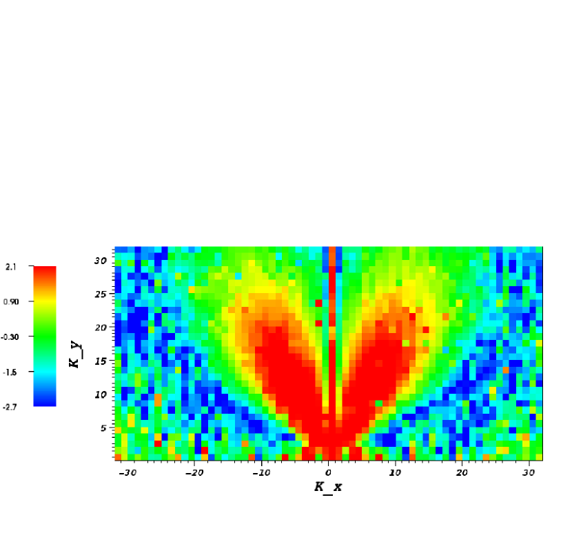
In the non-linear regime, Turner et al. (2005) found the instability produces shock trains that propagate from the bottom to the top of the atmosphere. With a purely horizontal background field, there is no preference for shocks propagating in either direction, resulting in a symmetric pattern of shocks in the atmosphere. The left panel of Figure 18 shows the density and velocity distribution at time $9.83$ when the shock train pattern becomes relatively strong. The velocity vectors are nearly horizontal direction because flow is confined to be parallel to the strong horizontal magnetic field. This figure can be compared with the first panel of Figure 19 of Turner et al. (2005): our results are very similar.

Figure 18.— Non-linear outcome of Photon Bubble instability at time $9.83$, corresponding to $1.56$ orbital periods. The left panel shows the density and velocity vectors. The right panel plots $\cos\theta$, where $\theta$ is the angle between the perturbed co-moving radiation flux and the gradient of the perturbed co-moving radiation energy density. Deviations of $\cos\theta$ from one near the shock fronts indicate the difference between the direction of the flux in our simulations versus the value assumed in FLD.

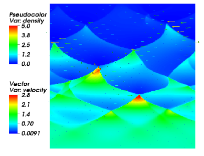
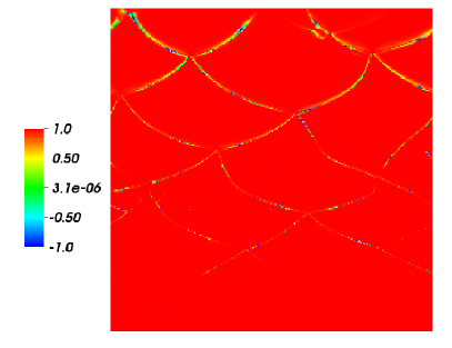
In the FLD approximation used by Turner et al. (2005), the co-moving radiation flux is always assumed to be along the direction of the gradient of the co-moving radiation energy density. Although we adopt the Eddington approximation in our simulation, we make no assumption about the direction of the flux. Thus, it is possible for us to test whether the radiation flux is indeed everywhere parallel to the gradient of $E_{r}$ in this highly nonlinear flow. Figure 18 shows the distribution of $\cos\theta$ at $t=9.83$, where the angle $\theta$ is the angle between the perturbed co-moving radiation flux in our simulation ${\mbox{\boldmath$F$}}_{r,0}-\hat{F}_{r,0}$ and the direction of the flux predicted by FLD $-{\mbox{\boldmath$\nabla$}}E_{r,0}/(3\sigma_{t})$. If the FLD approximation is valid, $\cos\theta$ will be one everywhere. We find that near the shock fronts, where there is a large density gradient, this assumption clearly fails. Since the optical depth across the domain is so large, the Eddington approximation should apply, and the flux-limiter used by Turner et al. (2005) should have a numerical value very close to the value of $1/3$ adopted here. Thus, the discrepancy in the direction of the radiation flux is not due to the value of the Eddington factor, but rather because in FLD the radiation flux is always along the gradient of radiation energy density.

6.5. Shadow Test

Since the direction of the flux is not known independently of the energy density, it is well-known that methods based on the diffusion approximation cannot represent shadows. This is often demonstrated through the irradiation of very optically thick structures with a beamed radiation field (e.g., Hayes & Norman, 2003; González et al., 2007). In this section, we demonstrate our methods capture shadows accurately, and moreover we present the dynamical evolution of a cloud ablated by an intense radiation field. VET is crucial to to get the solution correctly, which is calculated from the transfer module using short characteristic. The tests described in Davis et al. (2012) (see Figure 6 of that paper) show the accuracy of the radiation transfer solver for two radiation beams. Here we show that when coupled to the VET method, our solver captures shadows correctly.

Our test is performed in a rectangular box of size $(-0.5,0.5)\times(-0.3,0.3)$ cm. Initially the background medium has density $\rho_{0}=1$ $g/cm^{3}$ and temperature $T_{0}=290$ $K$. An over-dense clump is located in an elliptical region $r\equiv x^{2}/a^{2}+y^{2}/b^{2}\leq 1$, with $a=0.1$ $cm$ and $b=0.06$ $cm$. The density inside this region is $\rho(x,y)=\rho_{0}+(\rho_{1}-\rho_{0})/[1.0+\exp(10(r-1))]$ with $\rho_{1}=10\rho_{0}$. The clump is in pressure equilibrium with its surroundings, so the interior is much colder than the ambient medium. The initial radiation temperature is the same as the gas temperature everywhere. Pure absorption opacity is used with $\sigma=(T/T_{0})^{-3.5}(\rho/\rho_{0})^{2}$ $cm^{-1}$. The radiation flux ${\mbox{\boldmath$F$}}_{r}$ is zero everywhere initially. Outflow boundary conditions are used on both $y$ boundaries, and on the right $x$ boundary. A constant radiation field with temperature $T_{r}=6T_{0}$ is input through the left $x$ boundary at angles of $\pm 14$ degrees with respect to the $x$ axis. This radiation field is also input along the top $y$ boundary at $-14$ degrees, and along the bottom $y$ boundary at $+14$ degrees, in order to mimic the radiation field from an infinite plane along the left $x$ boundary at $x=-0.5$. At the left $x$ boundary, the gas temperature and density are fixed to $T_{0}$ and $\rho_{0}$ respectively. A resolution of $512\times 256$ cells is used for this test. The dimensionless speed of light ${\mathbb{C}}=1.9\times 10^{5}$, and the parameter ${\mathbb{P}}=2.2\times 10^{-15}$.

In the ambient medium, the photon mean free path is the length of simulation domain, so that the radiation can propagate freely across the box. However, inside the clump the photon mean free path is only $3.2\times 10^{-6}$ of the length of simulation box due to the high density and low temperature. Thus, radiation coming from the left boundary cannot penetrate the clump, and shadows are cast towards the right boundary. By using an input radiation field at two angles, both umbra and penumbra are formed. This makes the test more difficult, because ad-hoc closures that capture only one direction for the flux will not represent both the umbra and penumbra correctly.

In Figure 19 , we show the radiation energy density, and $x-x$ and $y-y$ components of the VET after one timestep at $\delta t=1.0e^{-3}$. This timestep corresponds to the CFL stability condition set by the adiabatic sound speed in the ambient gas and the grid resolution. The ratio of this timestep to the light crossing time of the domain is about 500, thus after one timestep both radiation beams have crossed the domain and a steady-state shadow structure is formed.

Figure 19.— Shadows created by the irradiation of an optically thick clump by two beams at $\pm 14$ degrees with respect to the $x$ axis. From top to bottom, the three panels show the radiation energy density $E_{r}$, and the $xx$ and $yy$ components of Eddington tensor $f_{xx}$ and $f_{yy}$ respectively. Inside the clump, the Eddington tensor is close to $1/3$ due to the large opacity, while $E_{r}$ retains its initial value. Umbra and penumbra are clearly formed behind the clump.

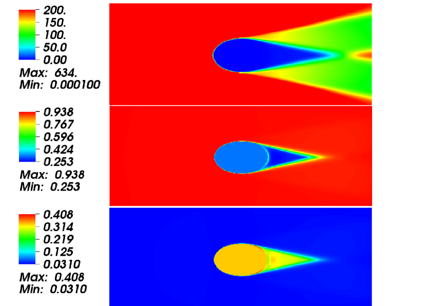
Since the radiation temperature is low in this first test, the clump undergoes negligible dynamical evolution. To demonstrate the dynamics of the ablation of a clump, we have repeated this test with an increase the background temperature $T_{0}$ by a factor of $357$ such that the dimensionless ${\mathbb{P}}=10^{-7}$. Then the radiation pressure of the applied radiation field at the left $x$ boundary is about $10^{-3}$ of the gas pressure. This non-negligible radiation field pushes and compresses the clump from the left and the shape of the clump is changed. A shock is driven into the clump during this process. The clump is also heated up by the radiation field and outflow from the surface of the clump is formed on the left side. The density distribution and velocity field at three different times are shown in Figure 20. The adiabatic sound speed in the ambient medium is $1.3$ in our units and $0.39$ inside the clump. In the first panel of Figure 20, the density on the left side of the clump is increased by a factor of $2$ due to the radiation pressure. Outflow is generated from the surface of the clump as shown by the velocity vectors. The flow is subsonic in the ambient medium and supersonic with respect to the sound speed inside the clump. In the second panel, we clearly see a shock driven to the clump with Mach number up to $3$. In the third panel, the clump is completely destroyed by the radiation field and several shock fronts are formed. The ablation of clouds by strong radiation field is in fact of great interest in the interstellar medium (ISM) (e.g., Bertoldi & McKee, 1990; Bally, 1995) and near the central region of quasars (e.g., Mathews, 1983). Further explore of this flow is warranted, but beyond the scope of this paper.

Figure 20.— Ablation of an optically thick clump by two radiation beams at $\pm 14$ degrees with respect to the $x$ axis. From top to bottom, the density (color) and velocity (vectors) are shown times $t=4.9\times 10^{-7},\ 1.3\times 10^{-6}$ and $2.6\times 10^{-6}s$ respectively.

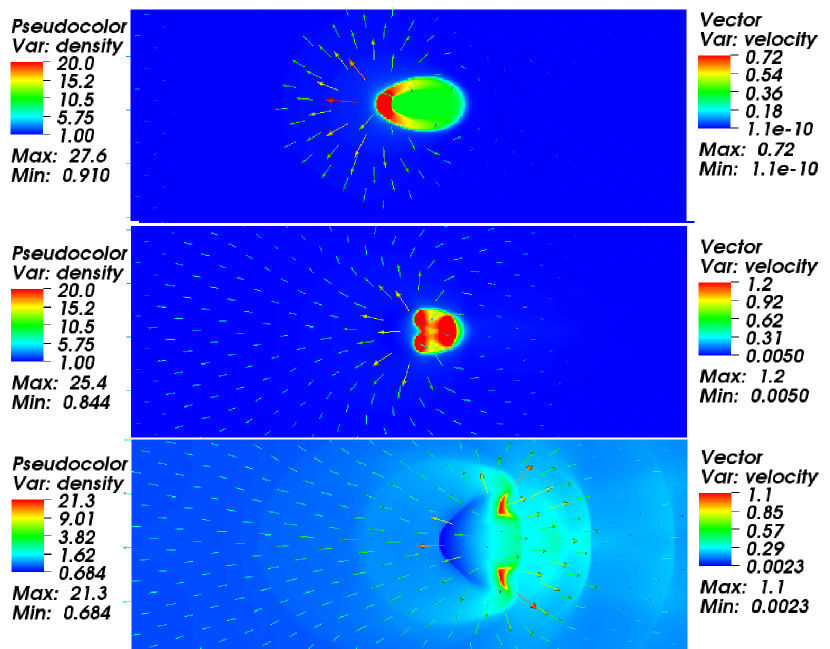
7. Discussion

7.1. Comparison with methods based on the diffusion approximation

A central ingredient of the algorithm presented in this paper is that it uses a VET to close the radiation moment equations, rather than relying on the diffusion approximation. It is therefore worthwhile to discuss specific examples where there will be differences between these approaches.

The first difference is that by solving the moment equations for the radiation flux, we are able to solve for the direction of the flux self-consistently with the flow, rather than assuming it lies in the direction of $\nabla E_{r}$. Both the photon bubble instability (see Figure 18) and the shadow test (see Figure 19) demonstrate the importance of keeping the direction of the flux.

A second difference is that the value of the flux limiter is always an approximation (of unknown reliability) to the true value of the diagonal components of the VET. In fact, the planar subcritical shock test (see Figure 15) shows that near the shock front, the VET can be less than $1/3$ along the direction of the radiation energy density gradient, which clearly cannot be represented by the formulae used for most limiters (e.g., Levermore & Pomraning, 1981). Based on the density distribution from a snapshot of simulations for black hole accretion disk done by Hirose et al. (2006), Davis et al. (2012) compares the Eddington tensor used in the flux-limited diffusion approximation and the VET calculated based on our transfer module. They also show significant difference (see Figure 7 of that paper). In the photosphere, the Eddington tensor given by the diffusion approximation can be much larger than the values given by the VET.

A third difference is that we do not drop the time-derivative of the flux $\partial F_{r}/\partial t$ in the moment equations for the flux. This term is important when the inertia of the radiation field is important, and dropping this term can lead to incorrect behavior in this regime. For example, consider a uniform medium with density $\rho=1$, absorption opacity $\sigma_{a}=10$ and scattering opacity $\sigma_{s}=10$ in thermal equilibrium ($E_{r}=T^{4}=1$ in our dimensionless units) with zero fixed fram radiation flux, and an initially uniform velocity along the $x$-direction $v_{0}=1$. Adopt values for the dimensionless speed of light ${\mathbb{C}}=100$ and parameter ${\mathbb{P}}=1000$, and use the Eddington approximation. In the diffusion approximation, because the radiation energy density is always uniform, the co-moving radiation flux will be always be zero and the system will always be in thermal equilibrium. However, this is not true if the $\partial{\mbox{\boldmath$F$}}_{r}/\partial t$ term is kept. Since the gas has a non-zero velocity with respect to the radiation field, the co-moving radiation flux is not zero, and there will be a drag force from the radiation field on the fluid. (a consequence of the fact that solutions to the equations of radiation hydrodynamic are not Galilean invariant). Because of the drag with the radiation field, momentum will be exchanged and the gas will be heated. In this example, this process can be described by

$$\frac{\partial(\rho{\mbox{\boldmath$v$}})}{\partial t} = \mathbb{P}\sigma_{t}\left({\mbox{\boldmath$F$}}_{r}-\frac{{\mbox{\boldmath$v$}}E_{r}+{\mbox{\boldmath$v$}}\cdot{\mbox{\boldmath$P$}}_{r}}{\mathbb{C}}\right),\$$

$$\frac{\partial{\mbox{\boldmath$F$}}_{r}}{\partial t} = -\mathbb{C}\sigma_{t}\left({\mbox{\boldmath$F$}}_{r}-\frac{{\mbox{\boldmath$v$}}E_{r}+{\mbox{\boldmath$v$}}\cdot{\mbox{\boldmath$P$}}_{r}}{\mathbb{C}}\right).$$ (44)

In solutions to these equations, $\rho$ and $E_{r}$ are unchanged while the change of velocity with time $t$ can be described by

$$v(t)=v_{0}\left(1-\frac{{\mathbb{C}}}{{\mathbb{C}}+4{\mathbb{P}}/(3{\mathbb{C}})}\right)\exp\left[-{\mathbb{P}}\sigma_{t}\left(\frac{{\mathbb{C}}}{{\mathbb{P}}}+\frac{4}{3{\mathbb{C}}}\right)t\right]+\frac{v_{0}{\mathbb{C}}}{{\mathbb{C}}+4{\mathbb{P}}/(3{\mathbb{C}})}.$$ (45)

We compare this analytic solution for this problem, and a numerical solution generated by our algorithms, in Figure 21. Our solutions captures this momentum exchange process accurately, which is not possible with flux-limited diffusion. The importance of this process is characterized by the parameter ${\mathbb{P}}/{\mathbb{C}}^{2}$, which measures the importance of momentum carried by the radiation field compared with the material momentum.

Figure 21.— Momentum exchange between radiation and material due to radiation drag. Red line is the analytic solution given by equation 45, while the black lines are our numerical solutions for normalized velocity and radiation flux. The solution reaches equilibrium when the co-moving radiation flux is zero. The velocity changes by $12\%$ in this example.

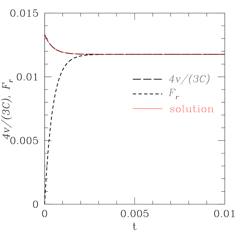
A fourth difference between our VET algorithm and FLD is that we keep the non-diagonal components of the VET. In the FLD approximation, the radiation pressure is always a diagonal tensor. Thus, radiation viscosity (e.g., Mihalas & Mihalas, 1984; Castor, 2004) cannot be captured in this approximation. However, with the VET approach, the off-diagonal components are computed self-consistently with the flow. Thus, the effects of radiation viscosity are captured naturally in simulations of accretion flows.

The importance of the differences between VET and FLD depend on the particular application of interest. For example, in the inner regions of accretion disks around supermassive black holes, we expect the momentum carried by the radiation field to be a significant fraction of material momentum (${\mathbb{P}}/{\mathbb{C}}^{2}$ is not negligible), and photon viscosity may be significant (e.g., Agol & Krolik, 1998). Thus, adopting algorithms based on VET is important for our applications.

7.2. Performance and Scaling

For solving the application problems of interest, our algorithms must not only be accurate, but also efficient. In this subsection, we report preliminary performance and scaling of the method on parallel systems. We continue to work on optimization of the algorithms, and it is likely substantial improvements in performance are still possible.

For reference, it is useful to compare to the performance of Athena in ideal MHD without radiation. On a single core of a $2.5$ GHz Intel Xeon processor, Athena updates roughly $1\times 10^{5}$ grid cells per second for 3D MHD calculations with a $32^{3}$ grid. Weak scaling is very good, with an efficiency (defined as the performance per core in a parallel calculation, compared to the performance of a serial calculation) of 0.9 on up to $10^{5}$ processors.

With radiation hydrodynamics and MHD, there are two potential bottlenecks. The first is the implicit solution of the linear radiation subsystem, which requires inverting one matrix per timestep (this is already an advantage over methods that require implicit solution of nonlinear systems which generally require many matrix inversions per timestep). To invert the matrix, we have explored the use of algorithms implemented in both the LIS (e.g., Nishida, 2010) and Hypre (e.g., Falgout et al., 2006) libraries, as well as our own implementation of the multigrid (e.g., Press et al., 1992) method. Both libraries provide a variety of iterative algorithms and preconditioners for solving sparse matrices, and can be used on both serial and parallel systems. The convergence rate of the matrix solver is limited by several things, such as the opacity and error tolerance.

To check the serial performance of each of these methods, we use the linear hydrodynamic wave problem as described in Section 6.1 on a 3D domain and a $32^{3}$ grid. With the LIS library on a single $2.5$ GHz Intel Xeon processor with tolerance level $10^{-8}$, we achieve roughly $1.7\times 10^{4}$ cell updates per cpu second in optical thick regimes with the ILU pre-conditioner. The Hypre library is somewhat faster, achieving about $3\times 10^{4}$ cell updates per cpu with the GMRES solver and the BoomerAMG preconditioner. Because the sparsity pattern of the matrix we invert is not common (see Appendix A), we must use the general matrix solvers in these libraries, which have very poor cache performance. By writing our own multigrid algorithm for inverting the matrix, we can take advantage of the specific structure of our matrix to substantially improve performance. With multigrid, we can achieve $4.3\times 10^{4}$ cell updates per cpu for this test, and the convergence rate is independent of whether the linear waves are optically thick or thin. With both the LIS and Hypre libraries, performance is about $2\sim 5$ times slower in the optically thin regime. Currently, the multigrid solver is our workhorse algorithm.

A second bottleneck to performance in simulations with radiation is the formal solution of the transfer equation. The cost of this step depends on the number of rays required to resolve the angular dependence of the radiation field, and whether the LTE approximation can be used to compute the source function (see Davis et al. 2012). In our tests, we have found sufficient accuracy is obtained with roughly 24 angles in 3D, although this number may be highly application dependent. If absorption opacity is dominant and the LTE approximation can be used, this step consumes a negligible fraction of the overall execution time. Moreover, since the cost to compute the VET scales linearly with the number of angles, using many more angles (for example, 80 instead of 24) does not affect the overall cost per timestep significantly. For example, using 80 angles increases the cost per timestep by less than factor of two compared to 24 angles.

However, if scattering opacity is dominant and the non-LTE integrator must be used to compute the VET, then this step can dominate the cost. With 24 angles in a non-LTE calculation, the overall performance of the code can be decreased by a factor of up to $5$. Moreover, using more angles decreases the convergence rate of the iteration scheme used for non-LTE problems, thus roughly tripling the number of angles (from 24 to 80) will increase the cost per timestep by more than a factor of three. There are several simple steps that can be used to increase performance in this regime, however. For example, in many cases it is possible to compute the VET only every several MHD time steps, since the geometry of the radiation field (and therefore the VET) changes only slowly compared to the flow structure.

It is interesting to compare the performance of the VET algorithm to FLD. Since we have not implemented FLD directly in Athena, we cannot perform a head-to-head comparison. However, we note that because the implicit differencing most often used with FLD (e.g., Turner & Stone, 2001; Zhang et al., 2011) involves nonlinear terms, Newton-Raphson iterations are required with one matrix solver per iteration. Depending on the convergence rate of the iterations, this could require several to many matrix solvers per timestep. Thus, Turner & Stone (2001) reported that in the optically thin limit the FLD module in ZEUS made the code run $10\times$ slower, whereas we find the VET algorithm (including the short-characteristics RT solver) is only $2-3\times$ slower than the standard MHD integrators in Athena. ZEUS itself is several times faster than Athena, so the VET may not in fact be faster than FLD, but it is at least comparable in performance. Using FLD because it is faster does not seem to be supported by these comparisons.

The parallel performance of the code is also limited by the matrix solver we use. Generally, in parallel calculations, the iterative linear system solver requires more steps to converge compared to the serial case. Using the linear hydrodynamic wave problem as described above, with $32^{3}$ grids on each processor, we have performed a weak scaling test for both the LIS and Hypre libraries, and our own multigrid solver. With 8 cores, the efficiency of the two libraries are about the same: $0.65$, and on 256 cores this drops to $0.25$. With our multigrid solver, the efficiency on 8 cores is $0.76$, and drops to $0.56$ on 256 cores. While this is substantially lower than the efficiency of the MHD integrator alone, it is still sufficient to enable large 3D applications. However, clearly further effort to improve performance is warranted.

8. Summary

We have described a Godunov algorithm for multidimensional radiation hydrodynamics and MHD, designed to study the dynamics of radiation dominated accretion flows around compact objects, and radiation driven winds from stars, disks, and galaxies. The algorithm has been implemented in the Athena MHD code (Stone et al., 2008), and tested over a wide range of parameter space.

Compared with previous algorithms for radiation hydrodynamics, there are several features of our approach that bear special mention.

Use of a VET rather than FLD. Most multidimensional algorithms for radiation hydrodynamics adopt the FLD approximation. However, this means that the direction of the radiation flux is lost, that the value of the flux is determined by an ad-hoc limiter, that the inertia of the radiation field is lost and that the off-diagonal components of the radiation pressure are assumed to be zero. We have shown through a variety of test problems that using methods based on a VET overcomes these limitations.

Formal solution of the transfer equation via short characteristics. To compute the VET, we discretize the specific intensity over many angles, and solve the transfer equation using short characteristics. While this has been deemed prohibitively expensive for 3D applications, advances in algorithms and hardware have overcome this difficulty. We find we can solve the transfer equation in full 3D using 24 angles at a cost that is no more than a single timestep of the MHD algorithm. We have also explored the use of Monte Carlo methods to compute the VET, and have found for our applications, short characteristics is substantially faster (Davis et al., 2012).

Use of Godunov methods for the underlying MHD solver. The VET method has been implemented previously in the ZEUS (e.g., Stone et al., 1992; Hayes & Norman, 2003), and TITAN (Gehmeyr & Mihalas, 1994) codes, however these methods used an operator split method with an artificial viscosity for shock capturing. Instead, we have adopted a higher-order Godunov method with a dimensionally unsplit integrator. Comparison of the structure of radiation modified shocks show the advantages of this approach. Since the addition of stiff source terms to Godunov methods is problematic, we extend the modified Godunov method of SS10 to multi-dimensions. We show this method results in accurate and stable evolution.

To test our algorithms, we have introduced a variety of quantitative test problems. We show the results of error convergence tests for linear radiation modified acoustic waves in both hydrodynamics and MHD over a wide range of parameters, and give examples of eigenmodes that can be used by others for testing. We also use the structure of radiating shocks in non-equilibrium diffusion computed using the methods outlined by Lowrie & Edwards (2008). Our algorithm reproduces the subtle changes in shock structure that occur as the Mach number is increased, even including very high Mach numbers where radiation pressure dominates the postshock flow. We also have performed multidimensional tests based on the photon bubble instability and shadowing.

There are still some limitations to our algorithms, which could be improved with future development. For example, we assume LTE, and our methods are limited to the grey approximation. Extension to multiple frequency bands requires analytic expressions for the interaction between different frequency bands in order to calculate the propagation operator used to update the stiff source terms. This is an important direction for future work. Our algorithm cannot propagate linear waves very well when absorption opacity is very large, in particular when $\tau_{a}>{\mathbb{C}}/{\mathbb{P}}$. Note that the algorithm is still capable of capturing flows in this regime. However, the damping rate and phase velocities of radiation modified acoustic waves will not be accurate. This can be improved by solving the total conservative form of the equations in this regime. If absorption opacity is so large that radiation temperature is locked to the gas temperature, the $\sigma_{a}(T^{4}-E_{r})$ term can be dropped in the radiation energy source term. Then damping rate and phase velocity of the radiation modified acoustic waves can be captured accurately in this regime. Since we solve the radiation transfer equations in the mixed-frame, our algorithm cannot be used for problems when spectral lines dominate the transport. The current algorithm is also not appropriate for problems when the radiation field changes rapidly (on a light-crossing time) because the VET is calculated using the time-independent transfer equation, although the error introduced by this assumption is acceptable if the time step is comparable to the light-crossing time of each cell, as we demonstrated in Section 5.2.

Not all the applications of interest requiring including the effects of radiation pressure. In this regime, it is possible to use a much simpler algorithm which only adds the radiation source terms to the energy equations, computed from a formal solution of the transfer equation. This method is described in a companion paper (Davis et al., 2012), and is currently being used to study black hole accretion disks in the gas pressure dominated regime. We use the same module for computing the VET in this work.

Currently we are using the radiation MHD version of Athena to study several applications, including the nonlinear regime of the Rayleigh-Taylor instability in a radiation supported atmosphere, radiation feedback in AGN, and the saturation of the magneto-rotational instability (MRI) in radiation dominated disks (Jiang et al. in preparation). Eventually the code will be publicly available through the Athena Trac site.

Appendix A Matrix for the 3D radiation subsystem

Implicit backward Euler differencing of the radiation subsystem (equation 36 and 37) results in a set of linear equations for the radiation energy density and flux in each cell. For every cell with indices $(i,j,k)$, we have the following four equations

$$\theta_{0}E_{r}^{n+1}(i,j,k-1)+\theta_{1}F_{r3}^{n+1}(i,j,k-1)$$

$$+ \theta_{2}E_{r}^{n+1}(i,j-1,k)+\theta_{3}F_{r2}^{n+1}(i,j-1,k)$$

$$+ \theta_{4}E_{r}^{n+1}(i-1,j,k)+\theta_{5}F_{r1}^{n+1}(i-1,j,k)$$

$$+ \theta_{6}E_{r}^{n+1}(i,j,k)+\theta_{7}F_{r1}^{n+1}(i,j,k)+\theta_{8}F_{r2}^{n+1}(i,j,k)+\theta_{9}F_{r3}^{n+1}(i,j,k)$$

$$+ \theta_{10}E_{r}^{n+1}(i+1,j,k)+\theta_{11}F_{r1}^{n+1}(i+1,j,k)$$

$$+ \theta_{12}E_{r}^{n+1}(i,j+1,k)+\theta_{13}F_{r2}^{n+1}(i,j+1,k)$$

$$+ \theta_{14}E_{r}^{n+1}(i,j,k+1)+\theta_{15}F_{r3}^{n+1}(i,j,k+1)$$

$$= E_{r}^{n}(i,j,k)-(1-\mathcal{R})dS_{r}(E)/{\mathbb{P}}+\mathcal{R}d_{2}\sigma_{a}\tilde{T}_{i,j,k}^{4},$$

$$\phi_{0}E_{r}^{n+1}(i,j,k-1)+\phi_{1}F_{r1}^{n+1}(i,j,k-1)$$

$$+ \phi_{2}E_{r}^{n+1}(i,j-1,k)+\phi_{3}F_{r1}^{n+1}(i,j-1,k)$$

$$+ \phi_{4}E_{r}^{n+1}(i-1,j,k)+\phi_{5}F_{r1}^{n+1}(i-1,j,k)$$

$$+ \phi_{6}E_{r}^{n+1}(i,j,k)+\phi_{7}F_{r1}^{n+1}(i,j,k)$$

$$+ \phi_{8}E_{r}^{n+1}(i+1,j,k)+\phi_{9}F_{r1}^{n+1}(i+1,j,k)$$

$$+ \phi_{10}E_{r}^{n+1}(i,j+1,k)+\phi_{11}F_{r1}^{n+1}(i,j+1,k)$$

$$+ \phi_{12}E_{r}^{n+1}(i,j,k+1)+\phi_{13}F_{r1}^{n+1}(i,j,k+1)$$

$$= F_{r1}^{n}(i,j,k)+d_{2}\sigma_{a}v_{x}\tilde{T}_{i,j,k}^{4}/\mathbb{C},$$

$$\psi_{0}E_{r}^{n+1}(i,j,k-1)+\psi_{1}F_{r2}^{n+1}(i,j,k-1),$$

$$+ \psi_{2}E_{r}^{n+1}(i,j-1,k)+\psi_{3}F_{r2}^{n+1}(i,j-1,k)$$

$$+ \psi_{4}E_{r}^{n+1}(i-1,j,k)+\psi_{5}F_{r2}^{n+1}(i-1,j,k)$$

$$+ \psi_{6}E_{r}^{n+1}(i,j,k)+\psi_{7}F_{r2}^{n+1}(i,j,k)$$

$$+ \psi_{8}E_{r}^{n+1}(i+1,j,k)+\psi_{9}F_{r2}^{n+1}(i+1,j,k)$$

$$+ \psi_{10}E_{r}^{n+1}(i,j+1,k)+\psi_{11}F_{r2}^{n+1}(i,j+1,k)$$

$$+ \psi_{12}E_{r}^{n+1}(i,j,k+1)+\psi_{13}F_{r2}^{n+1}(i,j,k+1)$$

$$= F_{r2}^{n}(i,j,k)+d_{2}\sigma_{a}v_{y}\tilde{T}_{i,j,k}^{4}/\mathbb{C},$$

$$\varphi_{0}E_{r}^{n+1}(i,j,k-1)+\varphi_{1}F_{r3}^{n+1}(i,j,k-1),$$

$$+ \varphi_{2}E_{r}^{n+1}(i,j-1,k)+\varphi_{3}F_{r3}^{n+1}(i,j-1,k)$$

$$+ \varphi_{4}E_{r}^{n+1}(i-1,j,k)+\varphi_{5}F_{r3}^{n+1}(i-1,j,k)$$

$$+ \varphi_{6}E_{r}^{n+1}(i,j,k)+\varphi_{7}F_{r3}^{n+1}(i,j,k)$$

$$+ \varphi_{8}E_{r}^{n+1}(i+1,j,k)+\varphi_{9}F_{r3}^{n+1}(i+1,j,k)$$

$$+ \varphi_{10}E_{r}^{n+1}(i,j+1,k)+\varphi_{11}F_{r3}^{n+1}(i,j+1,k)$$

$$+ \varphi_{12}E_{r}^{n+1}(i,j,k+1)+\varphi_{13}F_{r3}^{n+1}(i,j,k+1)$$

$$= F_{r3}^{n}(i,j,k)+d_{2}\sigma_{a}v_{z}\tilde{T}_{i,j,k}^{4}/\mathbb{C}.$$

Here $v_{x}$, $v_{y}$ and $v_{z}$ are the velocities along the $x-$, $y-$ and $z-$ directions respectively, and $d_{2}\equiv\Delta t\mathbb{C}$. The temperature $T^{r}_{i,j,k}$ is the value we estimate in Section 3.3.1. The velocities and opacity are at time step $n$ and are kept constant during the solution of the radiation moment equations.

Let the components of the symmetric $3\times 3$ VET ${\sf\boldmath f}$ be labelled as

$${\sf\boldmath f}=\left(\begin{array}[]{ccc}f_{11}&f_{12}&f_{13}\\ f_{21}&f_{22}&f_{23}\\ f_{31}&f_{32}&f_{33}\\ \end{array}\right).$$ (A5)

We also define the following quantities

$$d_{1x} \equiv \Delta t\mathbb{C}/(2\Delta x),\ d_{1y}\equiv\Delta t\mathbb{C}/(2\Delta y),\ d_{1z}\equiv\Delta t\mathbb{C}/(2\Delta z),$$ (A6)

$$Ci0 \equiv \frac{f_{11}^{1/2}(i,j,k)-f_{11}^{1/2}(i-1,j,k)}{f_{11}^{1/2}(i,j,k)+f_{11}^{1/2}(i-1,j,k)},\ Ci1\equiv\frac{f_{11}^{1/2}(i+1,j,k)-f_{11}^{1/2}(i,j,k)}{f_{11}^{1/2}(i+1,j,k)+f_{11}^{1/2}(i,j,k)},$$

$$Cj0 \equiv \frac{f_{22}^{1/2}(i,j,k)-f_{22}^{1/2}(i,j-1,k)}{f_{22}^{1/2}(i,j,k)+f_{22}^{1/2}(i,j-1,k)},\ Cj1\equiv\frac{f_{22}^{1/2}(i,j+1,k)-f_{22}^{1/2}(i,j,k)}{f_{22}^{1/2}(i,j+1,k)+f_{22}^{1/2}(i,j,k)},$$

$$Ck0 \equiv \frac{f_{33}^{1/2}(i,j,k)-f_{33}^{1/2}(i,j,k-1)}{f_{33}^{1/2}(i,j,k)+f_{33}^{1/2}(i,j,k-1)},\ Ck1\equiv\frac{f_{33}^{1/2}(i,j,k+1)-f_{33}^{1/2}(i,j,k)}{f_{33}^{1/2}(i,j,k+1)+f_{33}^{1/2}(i,j,k)}.$$

Then the coefficients $\theta_{0}-\theta_{15}$, $\phi_{0}-\phi_{13}$, $\phi_{0}-\phi_{13}$ and $\varphi_{0}-\varphi_{13}$ in equations A $-$ A are

$$\theta_{0} = -d_{1z}(1+Ck0)f_{33}^{1/2}(i,j,k-1),$$ (A7)

$$\theta_{1} = -d_{1z}(1+Ck0),$$

$$\theta_{2} = -d_{1y}(1+Cj0)f_{22}^{1/2}(i,j-1,k),$$

$$\theta_{3} = -d_{1y}(1+Cj0),$$

$$\theta_{4} = -d_{1x}(1+Ci0)f_{11}^{1/2}(i-1,j,k),$$

$$\theta_{5} = -d_{1x}(1+Ci0),$$

$$\theta_{6} = 1+d_{1x}(1+Ci1)f_{11}^{1/2}(i,j,k)+d_{1x}(1-Ci0)f_{11}^{1/2}(i,j,k)+d_{1y}(1+Cj1)f_{22}^{1/2}(i,j,k)$$

$$+ d_{1y}(1-Cj0)f_{22}^{1/2}(i,j,k)+d_{1z}(1+Ck1)f_{33}^{1/2}(i,j,k)+d_{1z}(1-Ck0)f_{33}^{1/2}(i,j,k)$$

$$+ \mathcal{R}d_{2}(\sigma_{a}-\sigma_{s})v_{x}\left[v_{x}(1+f_{11}(i,j,k))+v_{y}f_{12}(i,j,k)+v_{z}f_{13}(i,j,k)\right]/\mathbb{C}^{2}$$

$$+ \mathcal{R}d_{2}(\sigma_{a}-\sigma_{s})v_{y}\left[v_{y}(1+f_{22}(i,j,k))+v_{x}f_{12}(i,j,k)+v_{z}f_{23}(i,j,k)\right]/\mathbb{C}^{2}$$

$$+ \mathcal{R}d_{2}(\sigma_{a}-\sigma_{s})v_{z}\left[v_{z}(1+f_{33}(i,j,k))+v_{x}f_{13}(i,j,k)+v_{y}f_{23}(i,j,k)\right]/\mathbb{C}^{2}$$

$$+ \mathcal{R}d_{2}\sigma_{a},$$

$$\theta_{7} = d_{1x}(1+Ci1)-d_{1x}(1-Ci0)-\mathcal{R}d_{2}v_{x}(\sigma_{a}-\sigma_{s})/\mathbb{C},$$

$$\theta_{8} = d_{1y}(1+Cj1)-d_{1y}(1-Cj0)-\mathcal{R}d_{2}v_{y}(\sigma_{a}-\sigma_{s})/\mathbb{C},$$

$$\theta_{9} = d_{1z}(1+Ck1)-d_{1z}(1-Ck0)-\mathcal{R}d_{2}v_{z}(\sigma_{a}-\sigma_{s})/\mathbb{C},$$

$$\theta_{10} = -d_{1x}(1-Ci1)f_{11}^{1/2}(i+1,j,k),$$

$$\theta_{11} = d_{1x}(1-Ci1),$$

$$\theta_{12} = -d_{1y}(1-Cj1)f_{22}^{1/2}(i,j+1,k),$$

$$\theta_{13} = d_{1y}(1-Cj1),$$

$$\theta_{14} = -d_{1z}(1-Ck1)f_{33}^{1/2}(i,j,k+1),$$

$$\theta_{15} = d_{1z}(1-Ck1);$$

$$\phi_{0} = -d_{1z}(1+Ck0)f_{31}(i,j,k-1),$$ (A8)

$$\phi_{1} = -d_{1z}(1+Ck0)f_{33}^{1/2}(i,j,k-1),$$

$$\phi_{2} = -d_{1y}(1+Cj0)f_{21}(i,j-1,k),$$

$$\phi_{3} = -d_{1y}(1+Cj0)f_{22}^{1/2}(i,j-1,k),$$

$$\phi_{4} = -d_{1x}(1+Ci0)f_{11}(i-1,j,k),$$

$$\phi_{5} = -d_{1x}(1+Ci0)f_{11}^{1/2}(i-1,j,k),$$

$$\phi_{6} = d_{1x}(1+Ci1)f_{11}(i,j,k)-d_{1x}(1-Ci0)f_{11}(i,j,k)+d_{1y}(1+Cj1)f_{21}(i,j,k)$$

$$- d_{1y}(1-Cj0)f_{21}(i,j,k)+d_{1z}(1+Ck1)f_{31}(i,j,k)-d_{1z}(1-Ck0)f_{31}(i,j,k)$$

$$- d_{2}\sigma_{t}\left[v_{x}(1+f_{11}(i,j,k))+v_{y}f_{21}(i,j,k)+v_{z}f_{31}(i,j,k)\right]/\mathbb{C}+d_{2}\sigma_{a}v_{x}/\mathbb{C},$$

$$\phi_{7} = 1+d_{1x}(1+Ci1)f_{11}^{1/2}(i,j,k)+d_{1x}(1-Ci0)f_{11}^{1/2}(i,j,k)$$

$$+ d_{1y}(1+Cj1)f_{22}^{1/2}(i,j,k)+d_{1y}(1-Cj0)f_{22}^{1/2}(i,j,k)+d_{1z}(1+Ck1)f_{33}^{1/2}(i,j,k)$$

$$+ d_{1z}(1-Ck0)f_{33}^{1/2}(i,j,k)+d_{2}\sigma_{t},$$

$$\phi_{8} = d_{1x}(1-Ci1)f_{11}(i+1,j,k),$$

$$\phi_{9} = -d_{1x}(1-Ci1)f_{11}^{1/2}(i+1,j,k),$$

$$\phi_{10} = d_{1y}(1-Cj1)f_{21}(i,j+1,k),$$

$$\phi_{11} = -d_{1y}(1-Cj1)f_{22}^{1/2}(i,j+1,k),$$

$$\phi_{12} = d_{1z}(1-Ck1)f_{31}(i,j,k+1),$$

$$\phi_{13} = -d_{1z}(1-Ck1)f_{33}^{1/2}(i,j,k+1);$$

$$\psi_{0} = -d_{1z}(1+Ck0)f_{32}(i,j,k-1),$$ (A9)

$$\psi_{1} = -d_{1z}(1+Ck0)f_{33}^{1/2}(i,j,k-1),$$

$$\psi_{2} = -d_{1y}(1+Cj0)f_{22}(i,j-1,k),$$

$$\psi_{3} = -d_{1y}(1+Cj0)f_{22}^{1/2}(i,j-1,k),$$

$$\psi_{4} = -d_{1x}(1+Ci0)f_{21}(i-1,j,k),$$

$$\psi_{5} = -d_{1x}(1+Ci0)f_{11}^{1/2}(i-1,j,k),$$

$$\psi_{6} = d_{1x}(1+Ci1)f_{21}(i,j,k)-d_{1x}(1-Ci0)f_{21}(i,j,k)+d_{1y}(1+Cj1)f_{22}(i,j,k)$$

$$- d_{1y}(1-Cj0)f_{22}(i,j,k)+d_{1z}(1+Ck1)f_{32}(i,j,k)-d_{1z}(1-Ck0)f_{32}(i,j,k)$$

$$- d_{2}\sigma_{t}\left[v_{y}(1+f_{22}(i,j,k))+v_{x}f_{12}(i,j,k)+v_{z}f_{32}(i,j,k)\right]/\mathbb{C}+d_{2}\sigma_{a}v_{y}/\mathbb{C},$$

$$\psi_{7} = 1+d_{1x}(1+Ci1)f_{11}^{1/2}(i,j,k)+d_{1x}(1-Ci0)f_{11}^{1/2}(i,j,k)$$

$$+ d_{1y}(1+Cj1)f_{22}^{1/2}(i,j,k)+d_{1y}(1-Cj0)f_{22}^{1/2}(i,j,k)$$

$$+ d_{1z}(1+Ck1)f_{33}^{1/2}(i,j,k)+d_{1z}(1-Ck0)f_{33}^{1/2}(i,j,k)+d_{2}\sigma_{t},$$

$$\psi_{8} = d_{1x}(1-Ci1)f_{12}(i+1,j,k),$$

$$\psi_{9} = -d_{1x}(1-Ci1)f_{11}^{1/2}(i+1,j,k),$$

$$\psi_{10} = d_{1y}(1-Cj1)f_{22}(i,j+1,k),$$

$$\psi_{11} = -d_{1y}(1-Cj1)f_{22}^{1/2}(i,j+1,k),$$

$$\psi_{12} = d_{1z}(1-Ck1)f_{32}(i,j,k+1),$$

$$\psi_{13} = -d_{1z}(1-Ck1)f_{33}^{1/2}(i,j,k+1);$$

$$\varphi_{0} = -d_{1z}(1+Ck0)f_{33}(i,j,k-1),$$ (A10)

$$\varphi_{1} = -d_{1z}(1+Ck0)f_{33}^{1/2}(i,j,k-1),$$

$$\varphi_{2} = -d_{1y}(1+Cj0)f_{23}(i,j-1,k),$$

$$\varphi_{3} = -d_{1y}(1+Cj0)f_{22}^{1/2}(i,j-1,k),$$

$$\varphi_{4} = -d_{1x}(1+Ci0)f_{31}(i-1,j,k),$$

$$\varphi_{5} = -d_{1x}(1+Ci0)f_{11}^{1/2}(i-1,j,k),$$

$$\varphi_{6} = d_{1x}(1+Ci1)f_{31}(i,j,k)-d_{1x}(1-Ci0)f_{31}(i,j,k)+d_{1y}(1+Cj1)f_{32}(i,j,k)$$

$$- d_{1y}(1-Cj0)f_{32}(i,j,k)+d_{1z}(1+Ck1)f_{33}(i,j,k)-d_{1z}(1-Ck0)f_{33}(i,j,k)$$

$$- d_{2}\sigma_{t}\left[v_{z}(1+f_{33}(i,j,k))+v_{x}f_{31}(i,j,k)+v_{y}f_{32}(i,j,k)\right]/\mathbb{C}+d_{2}\sigma_{a}v_{z}/\mathbb{C},$$

$$\varphi_{7} = 1+d_{1x}(1+Ci1)f_{11}^{1/2}(i,j,k)+d_{1x}(1-Ci0)f_{11}^{1/2}(i,j,k)$$

$$+ d_{1y}(1+Cj1)f_{22}^{1/2}(i,j,k)+d_{1y}(1-Cj0)f_{22}^{1/2}(i,j,k)$$

$$+ d_{1z}(1+Ck1)f_{33}^{1/2}(i,j,k)+d_{1z}(1-Ck0)f_{33}^{1/2}(i,j,k)+d_{2}\sigma_{t},$$

$$\varphi_{8} = d_{1x}(1-Ci1)f_{31}(i+1,j,k),$$

$$\varphi_{9} = -d_{1x}(1-Ci1)f_{11}^{1/2}(i+1,j,k),$$

$$\varphi_{10} = d_{1y}(1-Cj1)f_{32}(i,j+1,k),$$

$$\varphi_{11} = -d_{1y}(1-Cj1)f_{22}^{1/2}(i,j+1,k),$$

$$\varphi_{12} = d_{1z}(1-Ck1)f_{33}(i,j,k+1),$$

$$\varphi_{13} = -d_{1z}(1-Ck1)f_{33}^{1/2}(i,j,k+1).$$

The above equations can be written in matrix form, with the vector of unknowns containing elements $(E_{r},F_{r1},F_{r2},F_{r3})^{n+1}_{i,j,k}$ with index $i$ varying fastest. The result is a large sparse banded matrix that must be inverted (see section 7.2). Note that some of the elements of the matrix depend on the boundary conditions. We have implemented periodic, reflecting, inflow and outflow conditions.

Appendix B Dispersion relation for linear waves in radiation hydrodynamics

In this appendix, we derive the dispersion relation for linear waves in radiation hydrodynamics used for the tests in section 6.1. The opacity $\sigma_{a}=\sigma_{t}=\sigma$ is a constant. The background state is chosen to be $\rho_{0}=1,P_{0}=1,E_{r,0}=1,T_{0}=1$, which is uniform with zero velocity and radiation flux, and is in mechanical and thermal equilibrium.

Following the analysis done by Johnson & Klein (2010), for each perturbed quantity, we look for wave solutions of the form $\delta\tilde{f}=\delta f\times\mathrm{e}^{\mathrm{i}(\omega t-kx)}$, where $k$ is the wave number, $\omega$ the angular frequency and $\delta f$ the amplitude. Note that we only need the real part of $\delta\tilde{f}$. The amplitude $\delta f$ can be a complex number, the imaginary part of which represents the relative phase shift between different quantities. Then the dispersion relation between $\omega$ and $k$ has the form

$$c_{4}k^{4}+c_{2}k^{2}+c_{0}=0,$$ (B1)

where the coefficients are

$$c_{4} = \mathrm{i}\frac{\gamma}{\gamma-1}\frac{\omega\mathbb{C}^{2}}{3\mathbb{P}\sigma}+\frac{4\mathbb{C}^{3}}{3},$$

$$c_{2} = -\mathrm{i}\frac{\mathbb{C}^{2}+3\gamma}{3\mathbb{P}\sigma(\gamma-1)}\omega^{3}-\left(\frac{4}{3}\mathbb{C}^{3}+\frac{2\mathbb{C}\gamma}{\mathbb{P}(\gamma-1)}+4\mathbb{C}+\frac{4\mathbb{C}}{9(\gamma-1)}\right)\omega^{2}$$

$$+ \mathrm{i}\left(\frac{\sigma\mathbb{C}^{2}\gamma}{\mathbb{P}(\gamma-1)}+\frac{20}{3}\mathbb{C}^{2}\sigma+\frac{16}{9}\mathbb{C}^{2}\mathbb{P}\sigma\right)\omega,$$

$$c_{0} = \mathrm{i}\frac{\omega^{5}}{\mathbb{P}\sigma(\gamma-1)}+\left(\frac{2\mathbb{C}}{\mathbb{P}(\gamma-1)}+\frac{4}{3\mathbb{C}(\gamma-1)}+4\mathbb{C}\right)\omega^{4}$$ (B2)

$$- \mathrm{i}\left(4\mathbb{C}^{2}\sigma+\frac{4\sigma}{3(\gamma-1)}+\frac{\mathbb{C}^{2}\sigma}{\mathbb{P}(\gamma-1)}+\frac{16\mathbb{P}\sigma}{3}\right)\omega^{3}.$$

Figure 22.— Solutions to the dispersion relation for linear waves in radiation hydrodynamics. The red lines are radiation diffusion modes, while the black lines are radiation modified acoustic waves. Both the phase velocity $V_{p}$ and damping rate per wavelength $L/\Lambda$ are shown. These solutions can be compared to Figures 101.4 and 101.5 of Mihalas & Mihalas (1984).

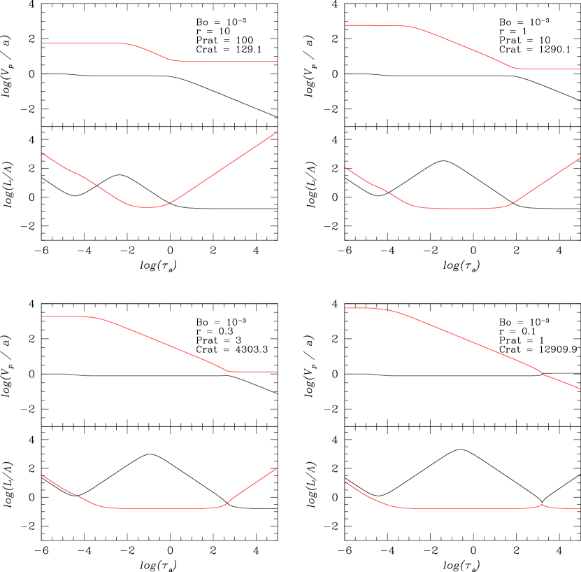
The dispersion relation is fourth order in the wave number $k$, and fifth order in the angular frequency $\omega$. It is identical to the dispersion relation given in equation 18 of Johnson & Klein (2010); although they use co-moving radiation energy density and radiation flux for their analysis, there is no difference for the linearized equations. The asymptotic behavior of the dispersion relation for different parameters $\sigma$ and ${\mathbb{P}}$ are discussed in detail by Bogdan et al. (1996) and Johnson & Klein (2010) and will not be repeated here. The analysis is done for a static background medium. Dispersion relation for a moving background medium is given by Lowrie et al. (1999). In particular, they point out that the radiation hydrodynamic system is not Galilean invariant. The damping rate of some radiation dominated modes depends on the flow velocity, because the co-moving radiation flux seen by the gas depends on the flow velocity.

In order to check that the dispersion relation we get is consistent with previous results, we reproduce Figures 101.4 and 101.5 of Mihalas & Mihalas (1984) in Figure 22. Those solutions are for boundary value problems, which means we assume a real number of angular frequency $\omega$ and calculate a complex wave number $k$. The dimensionless number Bo used in Mihalas & Mihalas (1984) is related to our dimensionless number ${\mathbb{P}}$ and ${\mathbb{C}}$ by equation (41) and another dimensionless number $r$ is determined by the following equation

$$r=\frac{(\gamma-1){\mathbb{P}}}{4\gamma}.$$ (B3)

The Boltzmann number Bo is a dimensionless number which measures the importance of energy flux carried by the radiation field. When $\text{Bo}\rightarrow\infty$, there is no energy exchange between radiation field and material. Equation 41 shows that the combination of our dimensionless numbers $1/({\mathbb{P}}{\mathbb{C}})$ has the same physical meaning. ${\mathbb{P}}$, or equivalent $r$, is a dimensionless number which measures the importance of momentum exchange between the radiation field and material, as discussed in section 6.1.

The dispersion relation given above must be solved using numerical root finding methods. For convenience, we give four numerical examples of eigenmodes that span the parameter space defined by ${\mathbb{P}}$ and $\sigma$ which can be used by others to test their own codes In all cases, ${\mathbb{C}}=10^{4}$ and $k=2\pi$.

Table 1Examples of solutions to the dispersion relation (B1)

${\mathbb{P}}$	0.01	0.01
$\sigma$	0.01	10
$\delta\rho$	$10^{-3}$	$10^{-3}$
$\delta v$	$1.27177\times 10^{-3}+8.15409\times 10^{-5}i$	$1.00012\times 10^{-3}+6.91295\times 10^{-6}i$
$\delta P$	$1.61075\times 10^{-3}+2.07402\times 10^{-4}i$	$1.00019\times 10^{-3}+1.36663\times 10^{-5}i$
$\delta E_{r}$	$1.79137\times 10^{-8}+8.56498\times 10^{-9}i$	$6.64619\times 10^{-7}+4.83820\times 10^{-5}i$
$\delta F_{r}$	$-1.32035\times 10^{-6}+3.88814\times 10^{-6}i$	$-9.99976\times 10^{-6}+1.40748\times 10^{-7}i$
$\omega$	$7.99077+0.512336i$	$6.28393+4.34354\times 10^{-2}i$
${\mathbb{P}}$	$100$	$100$
$\sigma$	$0.01$	$10$
$\delta\rho$	$10^{-3}$	$10^{-3}$
$\delta v$	$1.00000\times 10^{-3}+8.93099\times 10^{-8}i$	$9.99947\times 10^{-4}+1.07703\times 10^{-5}i$
$\delta P$	$1.00000\times 10^{-3}+1.57240\times 10^{-7}i$	$9.99998\times 10^{-4}+1.60499\times 10^{-7}i$
$\delta E_{r}$	$-3.55851\times 10^{-13}+6.41394\times 10^{-10}i$	$-6.60096\times 10^{-9}+6.41367\times 10^{-7}i$
$\delta F_{r}$	$-1.00000\times 10^{-9}+2.10690\times 10^{-13}i$	$-1.00130\times 10^{-9}+5.35966\times 10^{-11}i$
$\omega$	$6.28319+5.61151\times 10^{-4}i$	$6.28285+6.76716\times 10^{-2}i$
${\mathbb{P}}$	$100$	$1$
$\sigma$	$0.1$	$10$
$\delta\rho$	$10^{-3}$	$10^{-3}$
$\delta v$	$1.00000\times 10^{-3}+1.15555\times 10^{-7}i$	$1.00000\times 10^{-3}+3.32795\times 10^{-7}i$
$\delta P$	$1.00000\times 10^{-3}+1.73114\times 10^{-8}i$	$1.00000\times 10^{-3}+2.94229\times 10^{-7}i$
$\delta E_{r}$	$-1.0093\times 10^{-12}+6.41394\times 10^{-9}i$	$3.419000\times 10^{-10}+1.11408\times 10^{-6}i$
$\delta F_{r}$	$-1.00000\times 10^{-9}+5.51807\times 10^{-13}i$	$-1.00000\times 10^{-7}+1.22263\times 10^{-10}i$
$\omega$	$6.28319+7.26052\times 10^{-4}i$	$6.28319+2.09101\times 10^{-3}i$

Appendix C Dispersion relation for linear waves in radiation MHD

In this appendix, we derive the dispersion relation for linear waves in radiation MHD used for the tests in section 6.1. As in Appendix B, we assume a uniform, static background state, with a uniform magnetic field ${\mbox{\boldmath$B$}}_{0}=(B_{x,0},B_{y,0},B_{z,0})$. We assume the the wave propagation direction is along $x$ axis but the background magnetic field ${\mbox{\boldmath$B$}}_{0}$ can be along any direction. In general, $v_{x}$, $v_{y}$ and $v_{z}$ are all non-zero. The analysis proceeds as outlined in section B and will not be repeated here. In terms of the perturbed primitive variables $\delta{\mbox{\boldmath$W$}}=(\delta\rho,\delta v_{x},\delta v_{y},\delta v_{z},\delta P,\delta E_{r},\delta F_{r,x},\delta F_{r,y},\delta F_{r,z},\delta B_{y},\delta B_{z})^{T}$, the linearized equations can be written as $\mathbf{A}\delta{\mbox{\boldmath$W$}}=0$, where the coefficient matrix $\mathbf{A}$ is given in equation C1. The dispersion relation for radiation MHD waves is given by $det(\mathbf{A})=0$. This gives an eleventh order polynomial for $\omega$ and a tenth order polynomial for $k$. The solution can be simplified by assuming 2D solutions, in which ${\mbox{\boldmath$B$}}_{0}$, the wave vector, and all the perturbed quantities are on the same plane. In this case, the dispersion relation will be reduced to an eighth order polynomial for $\omega$ and a seventh order polynomial for $k$. The dispersion relation for radiation MHD waves including gravity in the short wavelength limit is discussed in detail by Blaes & Socrates (2003).

$$\scriptsize\left[\begin{array}[]{cccccccccccc}\omega&-k\rho_{0}&0&0&0&0&0&0&0&0&0\\ 0&\mathrm{i}\omega\rho_{0}+\frac{4}{3}\mathbb{P}\sigma\frac{E_{r,0}}{\mathbb{C}}&0&0&-\mathrm{i}k&0&-\mathbb{P}\sigma&0&0&-\mathrm{i}kB_{y,0}&-\mathrm{i}kB_{z,0}\\ 0&0&\mathrm{i}\omega\rho_{0}+\frac{4}{3}\mathbb{P}\sigma\frac{E_{r,0}}{\mathbb{C}}&0&0&0&0&-\mathbb{P}\sigma&0&\mathrm{i}kB_{x,0}&0\\ 0&0&0&\mathrm{i}\omega\rho_{0}+\frac{4}{3}\mathbb{P}\sigma\frac{E_{r,0}}{\mathbb{C}}&0&0&0&0&-\mathbb{P}\sigma&0&\mathrm{i}kB_{x,0}\\ \frac{4T_{0}^{4}}{\rho_{0}}\mathbb{P}\mathbb{C}\sigma&\mathrm{i}k\left(\frac{\gamma}{\gamma-1}P_{0}+B_{0}^{2}-B_{x,0}^{2}\right)&-\mathrm{i}kB_{x,0}B_{y,0}&-\mathrm{i}kB_{x,0}B_{z,0}&-\left(\frac{4T_{0}^{4}}{P_{0}}\mathbb{P}\mathbb{C}\sigma+\frac{\mathrm{i}\omega}{\gamma-1}\right)&\mathbb{P}\mathbb{C}\sigma&0&0&0&-\mathrm{i}\omega B_{y,0}&-\mathrm{i}\omega B_{z,0}\\ \frac{4T_{0}^{4}}{\rho_{0}}\mathbb{C}\sigma&0&0&0&-\frac{4T_{0}^{4}}{P_{0}}\mathbb{C}\sigma&\mathrm{i}\omega+\mathbb{C}\sigma&-\mathrm{i}k\mathbb{C}&0&0&0&0\\ 0&\frac{4}{3}\sigma E_{r,0}&0&0&0&\mathrm{i}k\frac{\mathbb{C}}{3}&-(\mathrm{i}\omega+\mathbb{C}\sigma)&0&0&0&0\\ 0&0&\frac{4}{3}\sigma E_{r,0}&0&0&0&0&-(\mathrm{i}\omega+\mathbb{C}\sigma)&0&0&0\\ 0&0&0&\frac{4}{3}\sigma E_{r,0}&0&0&0&0&-(\mathrm{i}\omega+\mathbb{C}\sigma)&0&0\\ 0&kB_{y,0}&-kB_{x,0}&0&0&0&0&0&0&-\omega&0\\ 0&kB_{z,0}&0&-kB_{x,0}&0&0&0&0&0&0&-\omega\\ \end{array}\right].$$ (C1)

For convenience, we give four numerical examples of eigenmodes for both slow and fast magnetosonic modes that span the parameter space defined by ${\mathbb{P}}$ and $\sigma$ which can be used by others to test their own codes. In all cases, ${\mathbb{C}}=10^{4}$ and $k=2\pi$.

Table 2Examples of solutions for radiation modified slow mode

${\mathbb{P}}$	0.01	0.01
$\sigma$	0.01	10
$\delta\rho$	$10^{-3}$	$10^{-3}$
$\delta v_{x}$	$7.77601\times 10^{-4}+5.56463\times 10^{-5}i$	$6.53191\times 10^{-4}+2.46133\times 10^{-6}i$
$\delta v_{y}$	$1.20178\times 10^{-3}+1.84722\times 10^{-4}i$	$8.77920\times 10^{-4}+5.58924\times 10^{-6}i$
$\delta P$	$1.52579\times 10^{-3}+2.97056\times 10^{-4}i$	$1.00009\times 10^{-3}+8.92617\times 10^{-6}i$
$\delta B_{y}$	$-7.15903\times 10^{-4}-1.63064\times 10^{-4}i$	$-4.44181\times 10^{-4}-4.50308\times 10^{-6}i$
$\delta E_{r}$	$1.54496\times 10^{-8}+1.02737\times 10^{-8}i$	$3.069869\times 10^{-7}+3.16009\times 10^{-5}i$
$\delta F_{r,x}$	$-1.89110\times 10^{-6}+3.34728\times 10^{-6}i$	$-6.53138\times 10^{-6}+6.48914\times 10^{-8}i$
$\delta F_{r,y}$	$1.61623\times 10^{-7}+1.67917\times 10^{-8}i$	$1.17056\times 10^{-7}+7.40429\times 10^{-10}i$
$\omega$	$4.88581+0.349636i$	$4.10401+1.54776\times 10^{-2}i$
${\mathbb{P}}$	$100$	$100$
$\sigma$	$0.01$	$10$
$\delta\rho$	$10^{-3}$	$10^{-3}$
$\delta v_{x}$	$6.53158\times 10^{-4}+3.18349\times 10^{-8}i$	$6.53158\times 10^{-4}+3.83780\times 10^{-6}i$
$\delta v_{y}$	$8.77864\times 10^{-4}+7.22107\times 10^{-8}i$	$8.77819\times 10^{-4}+8.70693\times 10^{-6}i$
$\delta P$	$1.00000\times 10^{-3}+1.02703\times 10^{-7}i$	$9.99999\times 10^{-4}+1.04836\times 10^{-7}i$
$\delta B_{y}$	$-4.44142\times 10^{-4}-5.81571\times 10^{-8}i$	$-4.44093\times 10^{-4}-7.01467\times 10^{-6}i$
$\delta E_{r}$	$-1.47792\times 10^{-13}+4.18932\times 10^{-10}i$	$-2.33054\times 10^{-9}+4.18933\times 10^{-7}i$
$\delta F_{r,x}$	$-6.53158\times 10^{-10}+9.61494\times 10^{-14}i$	$-6.53472\times 10^{-10}+2.36270\times 10^{-11}i$
$\delta F_{r,y}$	$1.16852\times 10^{-7}-4.78590\times 10^{-9}i$	$1.17043\times 10^{-7}+1.15612\times 10^{-9}i$
$\omega$	$4.10391+2.000251\times 10^{-4}i$	$4.10391+2.41136\times 10^{-2}i$
${\mathbb{P}}$	$100$	$1$
$\sigma$	$0.1$	$10$
$\delta\rho$	$10^{-3}$	$10^{-3}$
$\delta v_{x}$	$6.53158\times 10^{-4}+4.11763\times 10^{-8}i$	$6.53158\times 10^{-4}+1.18584\times 10^{-7}i$
$\delta v_{y}$	$8.77864\times 10^{-4}+9.34194\times 10^{-8}i$	$8.77865\times 10^{-4}+2.69043\times 10^{-7}i$
$\delta P$	$1.00000\times 10^{-3}+1.13071\times 10^{-8}i$	$1.00000\times 10^{-3}+1.92178\times 10^{-7}i$
$\delta B_{y}$	$-4.44142\times 10^{-4}-7.52612\times 10^{-8}i$	$-4.44142\times 10^{-4}-2.16754\times 10^{-7}i$
$\delta E_{r}$	$-3.78493\times 10^{-13}+4.18932\times 10^{-9}i$	$1.71921\times 10^{-10}+7.27673\times 10^{-7}i$
$\delta F_{r,x}$	$-6.53158\times 10^{-10}+2.43530\times 10^{-13}i$	$-6.53158\times 10^{-8}+5.44986\times 10^{-11}i$
$\delta F_{r,y}$	$1.17047\times 10^{-7}-4.67894\times 10^{-10}i$	$1.17049\times 10^{-7}+3.10689\times 10^{-11}i$
$\omega$	$4.10391+2.58718\times 10^{-4}i$	$4.10391+7.45083\times 10^{-4}i$

Table 3Examples of solutions for radiation modified fast mode.

${\mathbb{P}}$	0.01	0.01
$\sigma$	0.01	10
$\delta\rho$	$10^{-3}$	$10^{-3}$
$\delta v_{x}$	$2.08441\times 10^{-3}+2.26355\times 10^{-5}i$	$1.97671\times 10^{-3}+4.44472\times 10^{-6}i$
$\delta v_{y}$	$-1.29633\times 10^{-3}+3.15959\times 10^{-5}i$	$-1.47025\times 10^{-3}+8.22391\times 10^{-6}i$
$\delta P$	$1.64144\times 10^{-3}+1.30879\times 10^{-4}i$	$1.00104\times 10^{-3}+2.69749\times 10^{-5}i$
$\delta B_{y}$	$2.09358\times 10^{-3}-2.82848\times 10^{-5}i$	$2.25121\times 10^{-3}-7.53016\times 10^{-6}i$
$\delta E_{r}$	$1.89341\times 10^{-8}+7.85298\times 10^{-9}i$	$3.68258\times 10^{-6}+9.54978\times 10^{-5}i$
$\delta F_{r,x}$	$-8.33183\times 10^{-7}+4.08350\times 10^{-6}i$	$-1.97374\times 10^{-5}+7.74322\times 10^{-7}i$
$\delta F_{r,y}$	$-1.69620\times 10^{-7}+2.64650\times 10^{-8}i$	$-1.96034\times 10^{-7}+1.12087\times 10^{-9}i$
$\omega$	$13.0967+0.142223i$	$12.4200+2.79270\times 10^{-2}i$
${\mathbb{P}}$	$100$	$100$
$\sigma$	$0.01$	$10$
$\delta\rho$	$10^{-3}$	$10^{-3}$
$\delta v_{x}$	$1.97654\times 10^{-3}+5.75439\times 10^{-8}i$	$1.97651\times 10^{-3}+6.93247\times 10^{-6}i$
$\delta v_{y}$	$-1.47061\times 10^{-3}+1.06106\times 10^{-7}i$	$-1.47055\times 10^{-3}+1.28333\times 10^{-5}i$
$\delta P$	$1.00000\times 10^{-3}+3.10791\times 10^{-7}i$	$9.99999\times 10^{-4}+3.17242\times 10^{-7}i$
$\delta B_{y}$	$2.25153\times 10^{-3}-9.72688\times 10^{-8}i$	$2.25147\times 10^{-3}-1.17512\times 10^{-5}i$
$\delta E_{r}$	$-1.20333\times 10^{-12}+1.26774\times 10^{-9}i$	$-3.24677\times 10^{-9}+1.26773\times 10^{-6}i$
$\delta F_{r,x}$	$-1.97654\times 10^{-9}+1.11447\times 10^{-12}i$	$-1.97803\times 10^{-9}+2.44573\times 10^{-10}i$
$\delta F_{r,y}$	$-1.93101\times 10^{-7}+2.39955\times 10^{-8}i$	$-1.96073\times 10^{-7}+1.73546\times 10^{-9}i$
$\omega$	$12.4190+3.61559\times 10^{-4}i$	$12.4188+4.3558\times 10^{-2}i$
${\mathbb{P}}$	$100$	$1$
$\sigma$	$0.1$	$10$
$\delta\rho$	$10^{-3}$	$10^{-3}$
$\delta v_{x}$	$1.97654\times 10^{-3}+7.43855\times 10^{-8}i$	$1.97654\times 10^{-3}+2.14211\times 10^{-7}i$
$\delta v_{y}$	$-1.47061\times 10^{-3}+1.37659\times 10^{-7}i$	$-1.47061\times 10^{-3}+3.96547\times 10^{-7}i$
$\delta P$	$1.00000\times 10^{-3}+3.42168\times 10^{-8}i$	$1.00000\times 10^{-3}+5.81556\times 10^{-7}i$
$\delta B_{y}$	$2.25153\times 10^{-3}-1.26062\times 10^{-7}i$	$2.25153\times 10^{-3}-3.63108\times 10^{-7}i$
$\delta E_{r}$	$-1.52464\times 10^{-12}+1.26774\times 10^{-8}i$	$2.54552\times 10^{-9}+2.20203\times 10^{-6}i$
$\delta F_{r,x}$	$-1.97654\times 10^{-9}+2.53281\times 10^{-12}i$	$-1.97654\times 10^{-7}+5.86240\times 10^{-10}i$
$\delta F_{r,y}$	$-1.96050\times 10^{-7}+2.45310\times 10^{-9}i$	$-1.96081\times 10^{-7}+7.72241\times 10^{-11}i$
$\omega$	$12.4190+4.67378\times 10^{-4}i$	$12.419+1.34593\times 10^{-3}i$

References

- Agol & Krolik (1998) Agol, E., & Krolik, J. 1998, ApJ, 507, 304
- Arnett et al. (1989) Arnett, W. D., Bahcall, J. N., Kirshner, R. P., & Woosley, S. E. 1989, ARA&A, 27, 629
- Arons (1992) Arons, J. 1992, ApJ, 388, 561
- Balbus & Hawley (1998) Balbus, S. A., & Hawley, J. F. 1998, Reviews of Modern Physics, 70, 1
- Bally (1995) Bally, J. 1995, in Lecture Notes in Physics, Berlin Springer Verlag, Vol. 459, The Physics and Chemistry of Interstellar Molecular Clouds, ed. G. Winnewisser & G. C. Pelz, 118–119
- Bertoldi & McKee (1990) Bertoldi, F., & McKee, C. F. 1990, ApJ, 354, 529
- Blaes & Socrates (2001) Blaes, O., & Socrates, A. 2001, ApJ, 553, 987
- Blaes & Socrates (2003) —. 2003, ApJ, 596, 509
- Bogdan et al. (1996) Bogdan, T. J., Knoelker, M., MacGregor, K. B., & Kim, E. 1996, ApJ, 456, 879
- Bruls et al. (1999) Bruls, J. H. M. J., Vollmöller, P., & Schüssler, M. 1999, A&A, 348, 233
- Castor (2004) Castor, J. I. 2004, Radiation Hydrodynamics, ed. Castor, J. I.
- Castor (2009) Castor, J. I. 2009, in American Institute of Physics Conference Series, Vol. 1171, American Institute of Physics Conference Series, ed. I. Hubeny, J. M. Stone, K. MacGregor, & K. Werner, 230–241
- Ciotti & Ostriker (2007) Ciotti, L., & Ostriker, J. P. 2007, ApJ, 665, 1038
- Commerçon et al. (2011) Commerçon, B., Teyssier, R., Audit, E., Hennebelle, P., & Chabrier, G. 2011, A&A, 529, A35+
- Davis et al. (2012) Davis, S. W., Stone, J. M., & Jiang, Y.-F. 2012, ApJ
- Falgout et al. (2006) Falgout, R., Jones, J., & Yang, U. 2006, in Lecture Notes in Computational Science and Engineering, Vol. 51, Numerical Solution of Partial Differential Equations on Parallel Computers, ed. A. M. Bruaset & A. Tveito (Springer Berlin Heidelberg), 267–294, 10.1007/3-540-31619-1-8
- Gammie (1998) Gammie, C. F. 1998, MNRAS, 297, 929
- Gehmeyr & Mihalas (1994) Gehmeyr, M., & Mihalas, D. 1994, Physica D Nonlinear Phenomena, 77, 320
- Gentile (2001) Gentile, N. A. 2001, Journal of Computational Physics, 172, 543
- Gittings et al. (2008) Gittings, M., et al. 2008, Computational Science and Discovery, 1, 015005
- Gnedin & Abel (2001) Gnedin, N. Y., & Abel, T. 2001, New A, 6, 437
- González et al. (2007) González, M., Audit, E., & Huynh, P. 2007, A&A, 464, 429
- Hawley et al. (1995) Hawley, J. F., Gammie, C. F., & Balbus, S. A. 1995, ApJ, 440, 742
- Hayes & Norman (2003) Hayes, J. C., & Norman, M. L. 2003, ApJS, 147, 197
- Hirose et al. (2009) Hirose, S., Krolik, J. H., & Blaes, O. 2009, ApJ, 691, 16
- Hirose et al. (2006) Hirose, S., Krolik, J. H., & Stone, J. M. 2006, ApJ, 640, 901
- Janka et al. (2007) Janka, H.-T., Langanke, K., Marek, A., Martínez-Pinedo, G., & Müller, B. 2007, Phys. Rep., 442, 38
- Jiang & Goodman (2011) Jiang, Y.-F., & Goodman, J. 2011, ApJ, 730, 45
- Johnson & Klein (2010) Johnson, B. M., & Klein, R. I. 2010, J. Quant. Spec. Radiat. Transf., 111, 723
- Klein & Arons (1989) Klein, R. I., & Arons, J. 1989, in ESA Special Publication, Vol. 296, Two Topics in X-Ray Astronomy, Volume 1: X Ray Binaries. Volume 2: AGN and the X Ray Background, ed. J. Hunt & B. Battrick, 89–98
- Krumholz et al. (2007) Krumholz, M. R., Klein, R. I., McKee, C. F., & Bolstad, J. 2007, ApJ, 667, 626
- Krumholz et al. (2009) Krumholz, M. R., Klein, R. I., McKee, C. F., Offner, S. S. R., & Cunningham, A. J. 2009, Science, 323, 754
- Levermore & Pomraning (1981) Levermore, C. D., & Pomraning, G. C. 1981, ApJ, 248, 321
- Lowrie & Edwards (2008) Lowrie, R. B., & Edwards, J. D. 2008, Shock Waves, 18, 129
- Lowrie & Morel (2001) Lowrie, R. B., & Morel, J. E. 2001, J. Quant. Spec. Radiat. Transf., 69, 475
- Lowrie et al. (1999) Lowrie, R. B., Morel, J. E., & Hittinger, J. A. 1999, ApJ, 521, 432
- Marshak (1958) Marshak, R. E. 1958, Physics of Fluids, 1, 24
- Mathews (1983) Mathews, W. G. 1983, ApJ, 272, 390
- McKee & Ostriker (2007) McKee, C. F., & Ostriker, E. C. 2007, ARA&A, 45, 565
- Mihalas et al. (1978) Mihalas, D., Auer, L. H., & Mihalas, B. R. 1978, ApJ, 220, 1001
- Mihalas & Klein (1982) Mihalas, D., & Klein, R. I. 1982, Journal of Computational Physics, 46, 97
- Mihalas & Mihalas (1984) Mihalas, D., & Mihalas, B. W. 1984, Foundations of radiation hydrodynamics, ed. Mihalas, D. & Mihalas, B. W.
- Miniati & Colella (2007) Miniati, F., & Colella, P. 2007, Journal of Computational Physics, 224, 519
- Nishida (2010) Nishida, A. 2010, in Lecture Notes in Computer Science, Vol. 6017, Computational Science and Its Applications – ICCSA 2010, ed. D. Taniar, O. Gervasi, B. Murgante, E. Pardede, & B. Apduhan (Springer Berlin / Heidelberg), 448–462, 10.1007/978-3-642-12165-4-36
- Nordhaus et al. (2010) Nordhaus, J., Burrows, A., Almgren, A., & Bell, J. 2010, ApJ, 720, 694
- Offner et al. (2009) Offner, S. S. R., Klein, R. I., McKee, C. F., & Krumholz, M. R. 2009, ApJ, 703, 131
- Olson & Kunasz (1987) Olson, G. L., & Kunasz, P. B. 1987, J. Quant. Spec. Radiat. Transf., 38, 325
- Press et al. (1992) Press, W. H., Teukolsky, S. A., Vetterling, W. T., & Flannery, B. P. 1992, Numerical recipes in C. The art of scientific computing, ed. Press, W. H., Teukolsky, S. A., Vetterling, W. T., & Flannery, B. P.
- Proga (2007) Proga, D. 2007, ApJ, 661, 693
- Sekora & Stone (2010) Sekora, M. D., & Stone, J. M. 2010, Journal of Computational Physics, 229, 6819
- Shakura & Sunyaev (1973) Shakura, N. I., & Sunyaev, R. A. 1973, A&A, 24, 337
- Sincell et al. (1999) Sincell, M. W., Gehmeyr, M., & Mihalas, D. 1999, Shock Waves, 9, 391
- Spruit (2010) Spruit, H. C. 2010, ArXiv e-prints
- Stone et al. (2008) Stone, J. M., Gardiner, T. A., Teuben, P., Hawley, J. F., & Simon, J. B. 2008, ApJS, 178, 137
- Stone et al. (1992) Stone, J. M., Mihalas, D., & Norman, M. L. 1992, ApJS, 80, 819
- Su & Olson (1996) Su, B., & Olson, G. L. 1996, J. Quant. Spec. Radiat. Transf., 56, 337
- Swesty & Myra (2009) Swesty, F. D., & Myra, E. S. 2009, ApJS, 181, 1
- Trujillo Bueno & Fabiani Bendicho (1995) Trujillo Bueno, J., & Fabiani Bendicho, P. 1995, ApJ, 455, 646
- Turner et al. (2005) Turner, N. J., Blaes, O. M., Socrates, A., Begelman, M. C., & Davis, S. W. 2005, ApJ, 624, 267
- Turner & Stone (2001) Turner, N. J., & Stone, J. M. 2001, ApJS, 135, 95
- Turner et al. (2003) Turner, N. J., Stone, J. M., Krolik, J. H., & Sano, T. 2003, ApJ, 593, 992
- van der Holst et al. (2011) van der Holst, B., et al. 2011, ArXiv e-prints
- Vaytet et al. (2011) Vaytet, N. M. H., Audit, E., Dubroca, B., & Delahaye, F. 2011, J. Quant. Spec. Radiat. Transf., 112, 1323
- Zel’Dovich & Raizer (1967) Zel’Dovich, Y. B., & Raizer, Y. P. 1967, Physics of shock waves and high-temperature hydrodynamic phenomena, ed. Zel’Dovich, Y. B. & Raizer, Y. P.
- Zhang et al. (2011) Zhang, W., Howell, L., Almgren, A., Burrows, A., & Bell, J. 2011, ArXiv e-prints