Hard X-ray and UV Observations of the 2005 January 15 Two-ribbon Flare

Abstract

It is well known that two-ribbon flares observed in H$\alpha$ and ultraviolet (UV) wavelengths mostly exhibit compact and localized hard X-ray (HXR) sources (Warren & Warshall, 2001). In this paper, we present comprehensive analysis of a two-ribbon flare observed in UV 1600Å by TRACE and in HXRs by RHESSI. HXR (25 - 100 keV) imaging observations show two kernels of size (FWHM) 15″moving along the two UV ribbons. We find the following results. (1) UV brightening is substantially enhanced wherever and whenever the compact HXR kernel is passing, and during the hard X-ray transit across a certain region, the UV counts light curve in that region is temporally correlated with the hard X-ray total flux light curve. After the passage of the HXR kernel, the UV light curve exhibits smooth monotonical decay. (2) We measure the apparent motion speed of the HXR sources and UV ribbon fronts, and decompose the motion into parallel and perpendicular motions with respect to the magnetic polarity inversion line (PIL). It is found that HXR kernels and UV fronts exhibit similar apparent motion patterns and speeds. The parallel motion dominates during the rise of the HXR emission, and the perpendicular motion starts and dominates at the HXR peak, the apparent motion speed being 10 - 40 km s^-1. (3) We also find that UV emission is characterized by a rapid rise correlated with HXRs, followed by a long decay on timescales of 15 - 30 min. The above analysis provides evidence that UV brightening is primarily caused by beam heating, which also produces thick-target HXR emission. The thermal origin of UV emission cannot be excluded, but would produce weaker heating by one order of magnitude. The extended UV ribbons in this event are most likely a result of sequential reconnection along the PIL, which produces individual flux tubes (post-flare loops), subsequent non-thermal energy release and heating in these flux tubes, and then the very long cooling time of the transition region at the feet of these flux tubes.

1 INTRODUCTION

Solar flares are impulsive energy release events in the solar atmosphere. During flares, magnetic free energy is released by magnetic reconnection to accelerate particles, heat plasmas, and drive mass motions. Accelerated particles interacting with the lower solar atmosphere produce electromagnetic radiation at optical, ultraviolet (UV), and hard X-ray (HXR) wavelengths. By using multi-wavelength observations obtained from space telescopes, we can study various physical processes in flares.

Many studies have been focused on the temporal and spatial relationship between HXR and UV continuum emissions. Kane & Donnelly (1971) used HXR data from OGO satellites and ground-based sudden frequency deviation at 10-1030 Å, and showed similar time profiles at both wavelengths, particularly a strong temporal relationship during the rise of the flare. These studies provided observational evidence that HXR and UV emissions are associated with a common origin. Using data from SMM, Cheng et al. (1988) further studied the timing of HXR and UV broadband emissions, finding a strong temporal correlation between the two. They suggested that UV and HXR emissions are most likely produced by the same source particle population. They also provided evidence of localized UV and HXR sources through the UVSP images. Warren & Warshall (2001) suggested that the UV emission tends to exist in more extended ribbons while the HXR emission is generally more localized. Alexander & Coyner (2006) studied the flare on 2002 July 16 and concluded that the UV and HXR emissions are directly associated with the same flare energy release process, although the spatial separation existed. Furthermore, Coyner & Alexander (2009) conducted a statistical study focused on the relationship between the localized sources at both wavelengths and indicated two distinct types of UV emissions, one correlated with the HXR emission and the other more likely associated with a thermal origin.

The missing hard X-ray two-ribbon is a myth in solar flares. There are several possible reasons for the lack of HXR ribbons. First, it is suggested that energy release along the UV and optical ribbon is not uniform, and the dynamic range of the present HXR image reconstruction is about 10 (Sui et al., 2004), so energy deposition rate below one tenth of the maximum cannot be recovered in reconstructed HXR images. Second, either due to non-uniform energy release rate or due to the manner of energy release, namely, heating versus particle acceleration, particle acceleration may prefer to be localized. And last, energy release itself is localized and the UV or optical two-ribbons are a manifest of localized energy release sequentially along the ribbon and the elongated ribbon cooling time in UV or H$\alpha$ wavelength. In the last scenario, both of the hard X-ray and UV continuum emissions are thought to result from direct particle injection in the chromosphere. It has come to the recognition that even a two-ribbon flare is not 2-dimensional, but consists of numerous flare loops formed and energized individually by magnetic reconnection. Distinguishing the three different scenarios will provide important information of the form of energy release, namely, by direct heating or by particle acceleration, in these individual flare loops during the flare. Ideally, the best observational approach to distinguish the three scenarios is to spatially resolve electron deposit along flare loops, which may only have a cross-sectional area of around 1″. However, existing hard X-ray imaging capabilities are not able to resolve with such accuracy. Alternatively, high-resolution optical and UV imaging observations in combination with hard X-ray observations may be used to provide some spatial information of hard X-ray emissions. In this paper, we conduct a comprehensive quantitative analysis in order to shed light on this issue. The remainder of this paper is organized as follows. In §2 we briefly discuss the data analysis. We present the results in §3. Discussions and conclusions are made in §4.

2 Observations and Data Analysis

We present analysis of HXR and UV observations of an X2.6 flare on 2005 January 15. According to $Solar$ $Geophysical$ $Data$, the flare occurred from 22:25 UT to 23:31 UT in NOAA 720 when the active region was at the disk center. The longitudinal magnetograms of the active region were obtained by $Michelson$ $Doppler$ $Imager$ (MDI; Scherrer et al., 1995). The flare was observed, shortly after its onset, by the $Transition$ $Region$ $and$ $Coronal$ $Explorer$ (TRACE; Handy et al., 1999) in 1600 Å ultraviolet (UV) continuum with the best cadence (2 s) of the instrument and a pixel scale of 0.5″. Observations at this wavelength reflect the flare emission in the lower atmosphere, or emission at the feet of flaring loops. The $Reuven$ $Ramaty$ $High$ $Energy$ $Solar$ $Spectroscopic$ $Imager$ (RHESSI Lin et al., 2002) also observed the flare at X-ray wavelengths for its entire duration.

From RHESSI observations, we reconstruct HXR images with the PIXON method (Metcalf et al., 1996) in two energy ranges of 25-50 keV and 50-100 keV, to capture the non-thermal emission of the flare. Altogether 322 HXR images are reconstructed from 22:30:46.894 UT to 23:13:26.894 UT. The field of view of the reconstructed HXR maps is 256″$\times$ 256″with the spatial resolution 2″$\times$ 2″. The integral time to make HXR maps is taken to be 4 s, 8 s, or 12 s, depending on the observed counts rate during which the total integrated count rate is greater than 3000. The RHESSI maps and TRACE images are both coaligned with an SoHO/MDI magnetogram obtained before the flare.

To derive semi-quantitative information of UV emission, we look into the calibration of TRACE images. The TRACE 1600Å images are first processed using the ${\rm trace\_prep.pro}$ built in the SolarSoftWare (SSW), which performs dark current and flat field correction and exposure normalization. Figure 1, however, shows that the median $I_{m}(t)$ of the processed UV images, which is dominated by non-flaring quiescent regions, takes negative values at short exposures. Furthermore, the figure shows that $I_{m}(t)$ is inversely proportional to the exposure time $\tau_{exp}$, indicating that a dark current pedestal is not properly removed from the initial processing. We then obtain the dark current pedestal as the slope of the linear fit to the $I_{m}(t)\sim 1/\tau_{exp}$ scatter plot and remove it from the UV images (Qiu et al., 2010). With this first-order correction, the median of the UV emission is recovered, which varies between 250 and 350 counts per second. It is seen that there are still fluctuations in the corrected median light curve. We then discard the frames of UV images whose corrected median is different from the mean median by more than 2$\sigma$, where $\sigma$ is the standard deviation of the $I_{m}(t)\sim 1/\tau_{exp}$ fit. Such selection leaves 1313 out of 1350 frames of images for further analysis, so the cadence of the UV observations is not compromised. We further normalize each UV image to the median, namely, the UV counts rate in TRACE UV images is measured as how many times the quiescent median. Note that this first-order correction of the dark pedestal offset is not perfect, so there are still some remaining artifacts in the corrected light curves, such as some very short-lived spikes and dips in some low-count regions during the flare maximum.

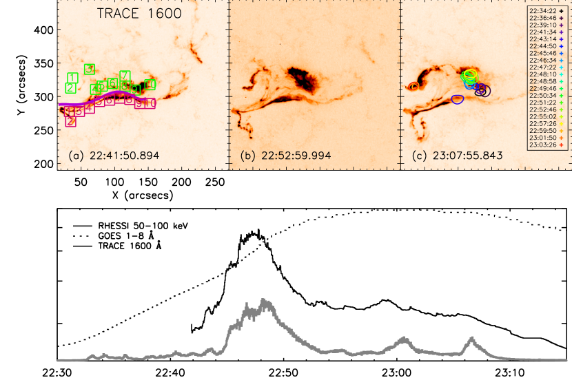
Figure 2 gives snapshots of the flare observed in UV and hard X-rays. TRACE 1600Å images show two flare ribbons along the magnetic polarity inversion line. The ribbon in the negative magnetic field (N-ribbon) appears to consist of two sections. The section in the west is brightened first, and the section in the east emits more strongly after 23:00 UT. HXR emission at 50-100 keV is primarily produced in one compact source S1, or hard X-ray kernel, located in the negative magnetic field. A very weak source S2, whose intensity is only about 10% of that of the strong source S1, is also visible in the positive magnetic field. The kernels are seen to “move” along the UV ribbon during the flare and are located at where UV emission is strong. Hard X-ray maps at 25-50 keV (not shown in the paper) show the same morphology and evolution pattern as the 50-100 keV sources. Therefore, in this flare, hard X-ray emission above 25 keV is considered to be thick-target non-thermal emission from the foot-points of flaring loops.

The bottom panel of the figure shows the corrected UV total counts light curve together with the RHESSI hard X-ray light curves at 50 - 100 keV, and the GOES soft X-ray light curve at 1-8 Å. It is seen that UV and HXRs rise, peak, and decay nearly simultaneously, suggesting the common origin of emissions at the two wavelengths. With the high cadence observations at the two wavelengths, we conduct detailed analysis to examine the temporal and spatial relationship between hard X-ray and UV emissions and the evolution pattern of hard X-ray and UV emissions.

3 Results

3.1 UV and HXR emissions

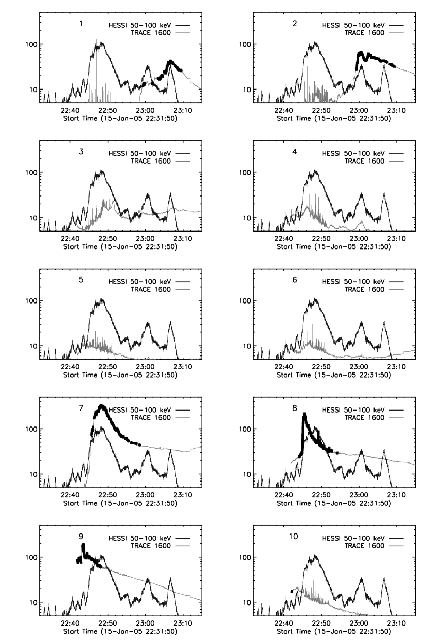
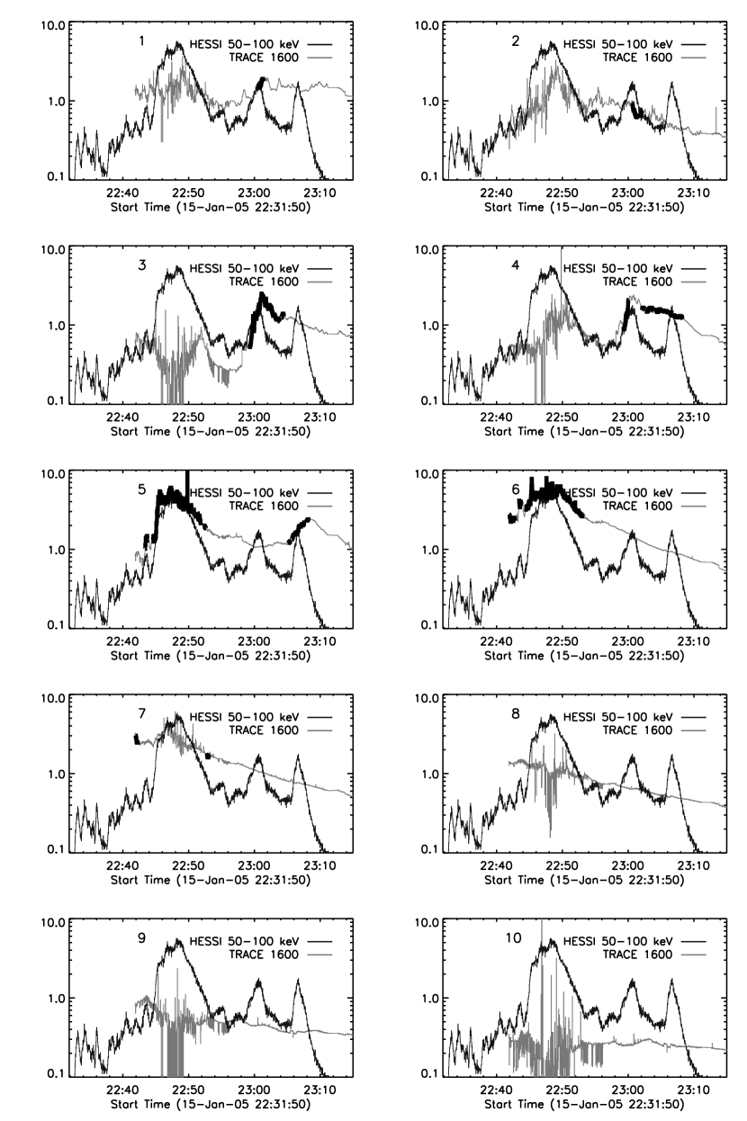
Figure 2 shows two flare ribbons in UV images and two kernels in hard X-ray emission. In order to investigate the spatial relationship between UV and HXR emissions, we compare the hard X-ray light curve with UV light curves in spatially resolved regions along the UV ribbons. For this purpose, we divide the UV flare ribbons into small boxes, each of size 15″$\times$ 15″. This is comparable with the FWHM of the HXR kernels which are approximately circular-shaped. These boxes are displayed in Figure 2. The boxes are selected in a left-right, top-bottom sequence, and different colors indicate boxes along the positive and negative ribbons, respectively. We compute the mean counts rate, normalized to the quiescent median, in each small box to obtain the TRACE light curves. The comparison of HXR and spatially resolved UV light curves is shown in Figure 3. In the figure, we denote on the UV light curve by thick dark lines the duration when the centroid of the HXR kernel falls into the box.

Figure 3 shows that, along both ribbons, when the HXR kernel passes through a specific part (box) of the UV ribbon, the UV light curve in that box rises rapidly with significant enhancement by one to two orders of magnitude over the pre-flare quiescent background. During the passage of the HXR kernel, the UV light curve in the box is well correlated with the HXR light curve. The peak UV enhancement in individual boxes is in general scaled with the HXR flux (except for box 9). If the HXR flux is very strong, there is a strong UV enhancement, otherwise, we observe a weak enhancement in the UV light curve. In each box, after the passage of the HXR kernel, the UV light curve exhibits a smooth monotonical decay.

In the negative magnetic field, at the beginning, the HXR kernel S1 is located at the western section of the N-ribbon. After 23:00 UT, the HXR source S1 shifts to the eastern section of the N-ribbon with much weaker emission. The HXR emission exhibits two small bursts after 23:00 UT. One is around 23:00 UT, another is at 23:07 UT, both coincident with brightened UV regions. We observe a similar pattern in the positive ribbon. When the HXR kernel S2 passes through a certain UV region, the UV light curve in that box shows significant enhancement, and it decays smoothly after the passage of S2. Note that the magnitude of UV enhancement in the P-ribbon is much smaller than in the N-ribbon by an order of magnitude, consistent with the relative intensities of two hard X-ray kernels.

The above comparison of hard X-ray light curve with spatially resolved UV light curves suggest that, along the ribbons, wherever and whenever HXR kernel passes, significant brightening will occur in the UV emission. Therefore, enhanced UV emission is primarily produced by precipitating electrons that also produce thick-target hard X-rays.

3.2 Evolution of HXR kernels and UV ribbons

The previous section shows that hard X-ray kernels move along the UV ribbons, and UV emission is strongest at the location of hard X-ray kernels. Such apparent motion is caused by reconnection and subsequent energy release along adjacent field lines along the ribbons. In this section, we examine in detail the apparent motion pattern of the energy deposit sites using hard X-ray as well as UV imaging observations.

Following the approach by Qiu (2009), we quantitatively characterize evolution of the flare ribbons and kernels with respect to the PIL. For this purpose, we first determine the profile of the PIL from the magnetogram, which is curved and extended nearly in the east to west direction. We then decompose the spread of ribbon brightening into two directions, parallel (elongation) and perpendicular (expansion) to the local PIL. To quantify the elongation and expansion of flare ribbons, we measure the following quantities for each ribbon at each time frame: the entire ribbon length ($l_{\|}$) projected along the PIL, and the mean distance ($d_{\bot}$) of the ribbon front perpendicular to the local PIL. The mean perpendicular distance $d_{\bot}$ is computed as $d_{\bot}$ = $S/l_{\|}$, where $S$ is the total area enclosed between the outer edge of the ribbon and the section of the PIL along the ribbon. The time profile of $l_{\|}$ gives a general description of the ribbon length growth along the PIL, whereas the time evolution of $d_{\bot}$ shows the separation of ribbon front away from the PIL.

In the similar way, we also decompose the trajectory of the centroid of each HXR kernel as components parallel and perpendicular to the PIL, respectively. The parallel distance of the centroid is measured from the same reference point where the UV ribbon starts, while the perpendicular distance refers to the distance of the centroid away from the PIL.

Figure 5 shows the parallel and perpendicular motion of the UV ribbon fronts as well as the HXR kernels. The analysis of the apparent ribbon motion is more ambiguous for the western section of the N-ribbon, which is brightened significantly after 23:00 UT, hence we only present the result for the eastern section of the N-ribbon before 23:00 UT. The N-ribbon elongates eastward along the PIL and moves away from the PIL, which is very well correlated with the motion of the HXR kernel S1. The maximum length of the negative UV ribbon ($l_{\|}$) can reach 40 Mm, with the average elongation speed of 40 km s^-1 from 22:42 UT to 22:49 UT. After that, the ribbon elongation slows down. The mean perpendicular distance (d_⊥) of the ribbon front varies from 14 Mm to 27 Mm with a mean speed of 22 km s^-1 between 22:43 UT to 22:49 UT and 8 km s^-1 afterwards.

The HXR kernel motion exhibits very similar trend. From 22:43:00 UT to 22:50:00 UT, the source S1 moves along the PIL from 7 Mm to 25 Mm with an average speed about 45 km s^-1. After that, there is no systematic parallel motion any more. The perpendicular motion starts several minutes later than the parallel motion. It begins at about 22:46 UT and lasts until 23:00 UT. The perpendicular motion can be divided into two phases. Before 22:52 UT, the perpendicular distance varies from 7 Mm to 15 Mm with a average speed about 22 km s^-1. After that, the perpendicular motion becomes slower and in the following 7 minutes, it moves only 5 Mm with a mean speed about 12 km s^-1.

The positive UV ribbon locates at the south of the PIL. Its trajectory is different from that of the negative ribbon. At the beginning, it spreads eastward along the PIL. After 22:48 UT, it moves back westward. The elongation motion pattern is similar to that of the HXR kernel S2, which moves eastward along the PIL from 2 Mm to 16 Mm with an average speed about 55 km s^-1 from 22:42 to 22:46 UT, and then moves back along the PIL with a mean speed about 35 km s^-1. Analysis of the UV ribbon also suggests a consistent perpendicular expansion motion away from the PIL at the average speed of 9 km s^-1. This is not seen in the HXR kernel S2 due to the very weak emission and therefore there is large uncertainty in determining the centroid of the kernel, as can be seen from the large fluctuation in the source position.

From the analysis above, we conclude that, first, the HXR sources and UV ribbon fronts show similar apparent motion patterns and motion speeds, further confirming the conclusion that hard X-ray emission and instantaneous UV brightening most likely come from the same location on the ribbon. On the other hand, spatially resolved UV emission exhibits a long smooth decay after the passage of HXR kernels. Therefore, our analysis suggests that, for this two-ribbon flare, the combined effect of elongation motion at the measured speed and the long decay time scale explains formation of the extended UV ribbons, whereas HXR emission appearing only as kernels may experience a much faster decay. The decay of UV emission will be further investigated in the next section. Second, it is seen that the parallel motion of the ribbon front or kernel dominates during the rise of HXR flux, whereas the perpendicular motion starts later and dominates during the peak of the HXR light curve, and continues into the decay of the HXR light curve. Such evolution pattern has been reported in a few flares (Moore et al., 2001; Qiu, 2009; Qiu et al., 2010).

3.3 Decay of UV emission

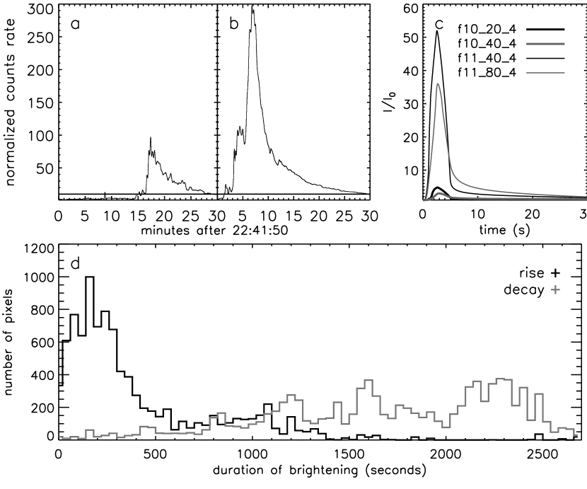
We further investigate the long decay seen in spatially resolved UV light curves in Figure 3. Such a long decay may be caused by very gradual cooling of the atmosphere that contributes to emission in the TRACE 1600Å band, or by continuous heating into the decay of the flare. Figure 6a shows the light curves of a few typical pixels in 1600Å, all demonstrating a rapid rise and a long decay. This was previously reported by Qiu et al. (2010) in the Bastille-day flare. However, for the Bastille-day flare, the TRACE observing cadence is low, of 30 - 40 seconds. The flare studied in this paper was observed with the highest cadence of 2 s, so that we can determine more precisely the rise and decay times of UV counts in each individual pixel.

In this paper, different from Qiu et al. (2010), we define the rise time as the time it takes for the counts rate in a pixel to rise from 10 times the quiescent median to the maximum, and the decay time is defined by the duration it takes for a pixel to decay from the maximum to 10 times the quiescent median. Empirically, the counts rate of 10 times the quiescent median is used as the criterion for flaring pixels (Qiu et al., 2010). The histograms of the so defined rise and decay times are shown in Figure 6d. It is seen that in individual flaring pixels, the rise time ranges from a few seconds to 4 minutes, whereas the typical “cooling” time is over 20 minutes, about an order of magnitude longer than the rise time. With this extended decay time and an average elongation speed of 40 km s^-1, the ribbon spreads to a length of over 40 Mm. This is comparable with the observed ribbon length. So, similar to Qiu et al. (2010), we conclude that the UV extended ribbon is a combined effect of energy release in flux tubes formed by reconnection sequentially along the PIL and the long decay of UV emission.

The elongated yet apparently smooth decay in UV emission may indicate a very long cooling process. To understand this, we employ the dynamic radiative transfer model to compute the time evolution of the lower atmosphere heated by non-thermal electrons with a power-law spectrum.

We perform radiative hydrodynamics modelling using the code RADYN (Carlsson & Stein, 1992, 1995, 1997, 2002) with application to solar flares as described in detail in Abbett (1998) and Abbett & Hawley (1999). Atoms important to the chromospheric energy balance are treated in non-LTE. We model hydrogen and singly ionized calcium with six-level atoms including the five lowest energy levels plus a continuum level. Singly ionized magnesium is described with a four-level model atom including the three lowest energy levels plus a continuum level. For helium we collapse terms to collective levels and include the $1s^{2}$, $2s$ and $2p$ terms in the singlet system and the $2s$ and $2p$ terms in the triplet system of neutral helium, and the $1s$, $2s$ and $2p$ terms of singly ionized helium. In addition we include doubly ionized helium. We include in detail all transitions between these levels. Complete frequency redistribution is assumed for all the lines except for the Lyman transitions, in which partial frequency redistribution is mimicked by truncating the profiles at 10 Doppler widths (Milkey & Mihalas, 1973). Other atomic species treated in LTE, are included in the calculations as background continua using the Uppsala opacity package of Gustafsson (1973). Optically thin radiative cooling due to bremsstrahlung and coronal metals is included in the equation of internal energy conservation via an additional cooling term.

The coupled, nonlocal, and nonlinear equations of radiative hydrodynamics, together with the charge conservation equation, are solved implicitly on an adaptive grid via Newton-Raphson iteration. The required linearization of the transfer equation follows the prescription of Scharmer (1981) and Scharmer & Carlsson (1985). The adaptive mesh is that of Dorfi & Drury (1987) and is of critical importance when modeling the dynamics of the lower atmosphere during flares. Features in the chromosphere, such as strong shocks and compression waves, develop quickly and require dense spatial distributions of grid points in order to be properly resolved. Even with the adaptive grid, it is necessary to use a total of 191 grid points (along with five angle points and up to 100 frequency points) to properly resolve important atmospheric features. Advected quantities are treated using the second-order upwind technique of van Leer (1977). Further details on the basic aspects of the numerical code can be found in Carlsson & Stein (1997, 1992) and Abbett (1998).

Then we compute the UV continuum radiation and convolves it with the TRACE 1600Å band response function. Figure 6c shows the computed count rates light curve as would be observed by TRACE 1600Å . These light curves are computed using different sets of electron parameters. The electron beam used in the simulation is defined by the peak non-thermal beam flux $f$, the electron power-law spectral index $\delta$, and the low cutoff energy $\epsilon_{cut}$. The simulation is conducted with $\delta=3,4,5$, $f=10^{9},10^{10},10^{11}$ ergs cm^-2 s^-1 (denoted as $f_{9}$, $f_{10}$, and $f_{11}$, respectively), and $\epsilon_{cut}=20,40,80$ keV, respectively. The time profile of the beam is a sinusoidal function with the rise and decay of 2.5 seconds each. The simulation shows that the result is least sensitive to changing $\delta$. The figure shows the computed counts rate light curve, normalized to the pre-flare quiescent intensity, for a few cases. It is seen that at $f=10^{11}$ ergs cm^-1 s^-1 and $\epsilon_{cut}=40$ keV, the maximum enhancement is one and half order of magnitude above the pre-flare emission. Furthermore, UV continuum emission rises nearly simultaneously with the beam with a delay less than 1 s, and the decay is almost as fast as the rise. With a strong beam of $\delta=4$, and $f=10^{11}$ ergs cm^-2 s^-1, the decay experiences a second gradual phase which lasts for a few minutes. Therefore, the continuum cooling is substantially faster than observed.

However, the computation does not take into account the C IV line which contributes significantly to the TRACE 1600Å band (Handy et al., 1998). The C IV line is a transition region line with a characteristic temperature of 100,000 K degree, and is therefore formed at transition region or low corona, which is heated during the flare. The long decay in the UV pixel is most likely dominated by “cooling” in the C IV line or the transition region, which cools down slowly due to maintained coronal pressure (Fisher et al., 1985; Hawley & Fisher, 1994; Griffiths et al., 1998) minutes after the initial energy deposit. The spectroscopic information is not available for this flare to study the contribution by the C IV line emission. However, spectroscopic observations of stellar flares have shown that C IV line emission dominates the decay phase of the flare emission, whereas the UV continuum radiation has significantly decreased (Hawley & Fisher, 1992).

3.4 Connectivity and Energetics

The results above suggest that magnetic reconnection and subsequent energy release take place in individual flux tubes other than in a 2.5-dimensional arcade structure as in the standard flare model. The brightest UV pixels at given times are most likely where instantaneous energy deposit takes place, and where hard X-ray emission is also produced. Like many other observations, in this flare, it is also seen that only two hard X-ray kernels are located, which are reasonably considered to be conjugate foot-points of newly formed flare loops. In the same spirit, we assume that the brightest UV kernels in the positive and negative magnetic fields are two conjugate foot-points of newly formed flare loops. The analysis reveals the apparent motion pattern of the kernels, which may reflect the changing orientation of the newly formed postflare loop. In this section, we study the orientation of the postflare loop, assumed to be determined by the inclination between the line connecting the conjugate footpoints and the local PIL.

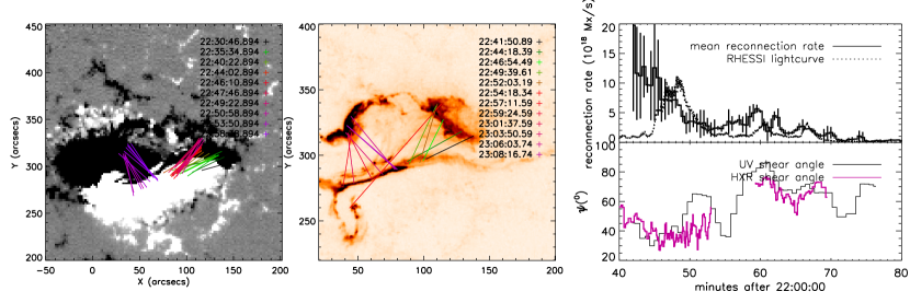
The left panel in Figure 7 illustrates the post-reconnection connectivity determined from HXR kernels, and the middle panel shows the post-reconnection connectivity determined from brightest UV emissions. The latter, with a much higher spatial resolution, would in principle yield a more accurate measurement of the positions of the kernels. We define the inclination angle of this projected post-reconnection loop with respect to the PIL as the shear angle $\psi$, and plot evolution of the shear angle in the right panel in Figure 7. A smaller $\psi$ indicates that the post-flare loop is more inclined toward the PIL, and a large $\psi$ indicates that the post-flare loop is more perpendicular to the PIL. It is seen that, in general, the evolution of the shear angle determined from HXR and UV kernels is consistent. In both plots, the shear angle continuously decreases toward the peak of HXR emission. Around the peak of HXR emission at 22:48 UT, the shear angle is smallest (40 degrees), indicating that the post-reconnection flare loop is most inclined toward the local PIL. After the peak, the shear angle increases and peaks during the decay phase, consistent with the observation that the apparent perpendicular motion proceeds into the decay phase whereas the parallel elongation motion has ceased. After the major HXR peak, it is seen that flare energy release takes place at a different location of the active region. The shear angle is greater, and gradually decrease towards HXR peaks around 23:00 UT. Therefore, there is a phenomenological relationship between flare non-thermal energetics and the orientation of the post-flare loop with respect to the local PIL.

A plausible explanation for the anti-correlation between the hard X-ray emission and the shear angle may involve a 3-dimentional reconnection configuration. In this scenario, reconnection takes place between two field lines that are not entirely anti-parallel but there is a component of the magnetic field along the reconnection current sheet or the polarity inversion line (e.g. Longcope et al., 2010). This current-aligned magnetic field component is the so-called guide field that does not change during reconnection. A stronger guide field would cause the post-reconnection loop more inclined toward the polarity inversion line, or smaller shear angle of the post-flare loop. The guide field present in the reconnection current sheet may trap electrons in the current sheet for longer time. If electrons are primarily accelerated by the reconnection electric field (e.g. Litvinenko, 1996), they may be accelerated for a longer time when there is a guide field. This scenario may explain why strong hard X-ray emission is related with small shear angle (large guide field).

The figure also shows the reconnection rate in terms of reconnection flux per unit time. The reconnection rate is measured by summing up magnetic flux in newly brightened UV pixels (Fletcher & Hudson, 2001; Qiu et al., 2004; Saba et al., 2006; Qiu et al., 2010). An automated procedure has been developed to identify flaring pixels and minimize measurement uncertainties caused by fluctuations in photometry calibration and by non-flaring signatures (Qiu et al., 2010). Displayed is the reconnection rate averaged in positive and negative fields. The vertical bars show the variations between the rates measured in positive and negative fields. For this flare, there is a large imbalance (30%) between positive and negative reconnection rates (Fletcher & Hudson, 2001). In this flare, since UV observations do not cover the early phase, we miss the rise phase of reconnection rate. The measurement shows that the reconnection rate peaks ahead of hard X-ray emission, and then decreases monotonically. Similar trend was reported in a few two-ribbon flares (Qiu, 2009; Qiu et al., 2010). It is noted that reconnection rate measurement takes into account magnetic flux in all newly brightened pixels. The large reconnection rate at the start of the flare is a result of a large number of flaring pixels before the peak of HXR emission. This is the stage when flare ribbon elongation dominates by kernels moving rapidly along the PIL. The lack of correlation between the reconnection rate and hard X-ray emission suggests that non-thermal energy release rate per unit reconnected flux is not uniform during the flare. During the phase of parallel motion, it appears that reconnection is not energetically favorable, similar to the conclusion by Qiu et al. (2010). The comparison suggests that, not only how much flux is reconnected, but also the pattern of reconnection, inferred from the kernel motion pattern and post-reconnection connectivity, governs the efficiency of non-thermal energy release (and therefore electron acceleration).

4 Conclusions

We analyze hard X-ray and UV observations of the two-ribbon flare on 2005 January 15 to examine the temporal and spatial relationship between emissions in these two wavelengths and to investigate how energy release is related to magnetic reconnection. The hard X-ray emission concentrates in two kernels in opposite magnetic fields whereas UV emission appears as two ribbons. The UV ribbon fronts and HXR kernels both exhibit apparent impulsive parallel motion and steady and slow perpendicular motion with respect to the magnetic PIL. It is evident that, along both ribbons, UV emission is impulsively enhanced when and where HXR kernel sweeps through. After the passage of the HXR kernel, UV emission decays gradually on timescales of over 20 minutes, apparently undergoing an elongated cooling. The analysis suggests that significant UV emission is primarily produced by non-thermal beam deposit which also produces hard X-ray emission. When such relationship can be established, it is possible to measure the area of non-thermal electron precipitation more precisely by combining high-resolution imaging UV observations with hard X-ray observations. This will provide an observational constraint on non-thermal beam parameters, such as the beam flux.

Furthermore, the observations of apparent motion of instantaneous energy release location and the long cooling time of UV emission provide an explanation for the apparent morphological discrepancy in the two wavelengths, that UV emission appears as extended ribbons whereas hard X-ray emission appears as compact kernels. These results support the scenario that reconnection and subsequent energy release takes place in individual flux tubes nearly sequentially along the magnetic polarity inversion line. The observations of this two-ribbon flare therefore presents the picture of 3D reconnection different from the 2.5D arcade configuration in the standard flare model.

It is also observed that the apparent parallel motion of the hard X-ray kernels and UV fronts dominates during the rise phase of hard X-ray emission, when reconnection rate peaks, and perpendicular motion dominates around the peak of the emission, when non-thermal energy flux is thought to reach maximum. With a 2.5D approximation, we also infer the inclination of the newly formed post-flare loops with respect to the PIL. The analysis shows the the shear angle of the postflare loop with respect to the PIL is smallest during the hard X-ray emissions, consistent with the motion pattern observed during the evolution of the flare. These observations suggest that efficiency of non-thermal energy release (in terms of non-thermal energy flux per unit reconnected flux) is related to the manner of reconnection as inferred from the inclination of newly formed post-flare loops. It is likely that the amount of magnetic energy release per unit reconnection flux is different depending on the shear change from the pre-flare to post-flare configuration. It is, however, also plausible that the inclination of post-flare loops indicates existence of a guide field component in the reconnection (Qiu et al., 2010). The guide field is the magnetic field component in the current sheet that is parallel with the reconnection electric field and does not participate in reconnection. Existence of the guide field modifies reconnection physics, and is particularly important in particle energization (e.g.; Litvinenko, 1996), which may be reflected in the observed phenomenological relationship between reconnection (apparent motion) pattern and non-thermal energetics. In this scenario, evolution of the shear angle is determined by pre-reconnection magnetic field configuration, such that low-lying field lines that reconnect earlier are becoming less sheared, and then the overlying field lines that reconnect later are more sheared, as shown in the cartoon in Figure 8.

Finally, we have also conducted the dynamic radiative transfer simulation to investigate evolution of UV continuum emission produced by non-thermal beams with varying beam parameters. It is found that the UV continuum emission time profile follows closely the heating function, which decays rapidly as soon as the heating terminates. The elongated cooling observed in the TRACE 1600Å band emission most likely reflects the transition region emission in the C IV line. In the future work, the C IV line contribution will be computed to provide a better guide in diagnosing radiative signatures observed in TRACE 1600 Å band. This will aide the analysis of energetics in flux tubes formed and energized by reconnection.

We thank Drs. R. W. Nightingale and T. Tarbell for help with TRACE calibration. We acknowledge TRACE, SoHO, and RHESSI missions for providing quality observations. This work is supported by NASA grant NNX08AE44G and NSF grant ATM-0748428. Part of the work was conducted during the NSF REU program at Montana State University and supported by Dr. D. E. McKenzie.

Figure 1: Left: the plot of uncorrected median values of UV counts rate versus 1/$\tau_{exp}$ (see text). Right: corrected UV median counts rate light curve.

Figure 2: Upper: Snapshots of the X2.6 flare observed by TRACE 1600 Å on 2005 January 15. The magnetic polarity inversion line is outlined by the purple line in the left panel. The boxes in the left panel indicate regions where spatially resolved UV counts rate light curves are obtained. In the right panel, the RHESSI HXR maps in 50-100 keV are overlayed. Bottom: Light curves for the flare in different energy bands.

Figure 3: The corrected TRACE UV counts rate light curves (grey) in small boxes as indicated in Figure 2 (N-ribbon), compared with HXR 50-100 keV count flux light curve (dark) arbitrarily normalized. The thick dark color on a TRACE light curve shows the timing when the HXR source passes through a certain box.

Figure 4: The corrected TRACE UV counts rate light curves (grey) in small boxes as indicated in Figure 2 (P-ribbon), compared with HXR 50-100 keV count flux light curve (dark) arbitrarily normalized. The thick dark color on a TRACE light curve shows the timing when the HXR source passes through a certain box.

Figure 5: Parallel (left panels) and perpendicular (right panels) distances of the HXR kernels and UV ribbon fronts with respect to the polarity inversion line. The upper panels show the motion of the HXR kernel S1 and UV N-ribbon, and the lower panels show the motion of the HXR kernel S2 and UV P-ribbon. The solid dark line shows the hard X-ray light curve at 100 - 300 keV as a reference.

Figure 6: Top left: corrected UV counts rate light curves in individual pixels. Top right: computed UV counts rate light curves (see text) with varying electron parameters. $f10\_20\_4$ indicates the electron beam of intensity $f=10^{10}$ ergs s ^-1 cm^-2, electron lower energy cutoff $\epsilon=$ 20 keV and electron spectral index $\delta=4$. Bottom: histograms of rise and decay times of UV emissions in 8000 flaring pixels.

Figure 7: Left: Conjugate HXR footpoints overlayed on the MDI magnetogram. Middle: conjugate UV footpoints overlayed on a TRACE image. Right (bottom): the shear angle of newly formed post-flare loops inferred from HXR (purple) and UV (black) sources, respectively. Right (up): the HXR flux in 50-100 keV (dotted line), and the reconnection rate (solid line). Vertical bars on the reconnection rate plot indicates uncertainties in the measurement.

Figure 8: A sketch of the possible post-flare loop arcade configuration, giving the top view of the sequentially formed post-flare loops. Low-lying loops (indicated in the figure as loops 1, 2, and 3) are formed earlier along the arcade, with the shear with the polarity inversion line (dashed line) decreasing with time. High-lying loops (loops 4 and 5) are formed later with increasing shear. The two arrows indicate the observed ribbon motion direction. The configuration explains the observed dominant parallel motion of the flare ribbon during the rise phase and the dominant perpendicular motion afterwards.

References

- Abbett (1998) Abbett, W. P. 1998, Ph.D. thesis, Michigan State Univ.
- Abbett & Hawley (1999) Abbett, W. P., & Hawley, S. L. 1999, ApJ, 521, 906
- Alexander & Coyner (2006) Alexander, D., & Coyner, A. J. 2006, ApJ, 640, 505
- Carlsson & Stein (1992) Carlsson, M., & Stein, R. F. 1992, ApJ, 397, L59
- Carlsson & Stein (1995) Carlsson, M., & Stein, R. F. 1995, ApJ, 440, 29
- Carlsson & Stein (1997) Carlsson, M., & Stein, R. F. 1997, ApJ, 481, 500
- Carlsson & Stein (2002) Carlsson, M., & Stein, R. F. 2002, ApJ, 572, 626
- Cheng et al. (1988) Cheng, C. C., Vanderveen, K., Orwig, L. E., & Taudberg-Haussen, E. 1988, ApJ, 330, 480
- Coyner & Alexander (2009) Coyner, A. J., & Alexander, D. 2009, ApJ, 705, 554
- Dorfi & Drury (1987) Dorfi, E. A., & Drury, L. O. 1987, J. Comput. Phys., 69, 175
- Fisher et al. (1985) Fisher, G. H., Canfield, R. C., McClymont, A. N., 1985, ApJ, 289, 425
- Fletcher & Hudson (2001) Fletcher, L., & Hudson, H. 2001, Sol. Phys., 204, 69
- Griffiths et al. (1998) Griffiths, N. W., Fisher, G. H., Siegmund, O. H. W. 1998, Cool Stars, Stellar Systems and the Sun, ASP Conference Series, Vol. 154, CD-621, eds. R. A. Donahue and J. A. Bookbinder
- Gustafsson (1973) Gustafsson, B. 1973, A FORTRAN Program for Calculating “ Continuous ” Absorption Coefficients of Stellar Atmospheres (Uppsala: Landstingets Vergstader)
- Handy et al. (1998) Handy, B. N., et al. 1998, Sol. Phys., 183, 29
- Handy et al. (1999) Handy, B. N., et al. 1999, Sol. Phys., 187, 229
- Hawley & Fisher (1994) Hawley, S. L., & Fisher, G. H. 1994, ApJ, 426, 387
- Hawley & Fisher (1992) Hawley, S. L., & Fisher, G. H. 1992, ApJS, 78, 565
- Kane & Donnelly (1971) Kane, S. R., & Donnelly, R. F. 1971, ApJ, 164, 151
- Lin et al. (2002) Lin, R. P., et al. 2002, Sol. Phys., 210, 3.
- Litvinenko (1996) Litvinenko, Y. E. 1996, ApJ, 462, 997
- Longcope et al. (2010) Longcope, D., Des Jardins, A., Carranza-Fulmer, T., Qiu, J., 2010, Solar Physics, 267, 107
- Metcalf et al. (1996) Metcalf, T. R., Hudson, H. S., Kosugi, T., Puetter, R. C., & Pima, R. K. 1996, ApJ, 466, 585
- Milkey & Mihalas (1973) Milkey, R. W., & Mihalas, D. 1973, ApJ, 185, 709
- Moore et al. (2001) Moore, Ronald L., Sterling, Alphonse C., Hudson, H. S., & Lemen, J. R. 2001, ApJ, 552, 833
- Qiu et al. (2004) Qiu, J., Wang, H., Cheng, C. Z., & Gary, Dale E. 2004, ApJ, 604, 900
- Qiu (2009) Qiu, J. 2009, ApJ, 692, 1110
- Qiu et al. (2010) Qiu, J., Liu, W. J., Hill, N., & Kazachenko, M. 2010, ApJ, 725, 319
- Saba et al. (2006) Saba, J. L. R., Gaeng, T., & Tarbell, T. D. 2006, ApJ, 641, 1197
- Scherrer et al. (1995) Scherrer, P. H., et al. 1995, Sol. Phys., 162, 129
- Scharmer (1981) Scharmer, G. B. 1981, ApJ, 249, 720
- Scharmer & Carlsson (1985) Scharmer, G. B., & Carlsson, M. 1985, J. Comput. Phys., 59, 56
- Smith et al. (2002) Smith, D. M., et al. 2002, Sol. Phys., 210, 33
- Sui et al. (2004) Sui, L., Holman, G. D., & Dennis, B. R. 2004, ApJ, 612, 546
- Warren & Warshall (2001) Warren, H. P., & Warshall, A. D. 2001, ApJ, 560, 87
- van Leer (1977) van Leer, B. 1977, J. Comput. Phys., 23, 276