Radio stacking reveals evidence for star formation in the host galaxies of X-ray selected active galactic nuclei at
Abstract
Nuclear starbursts may contribute to the obscuration of active galactic nuclei (AGNs). The predicted star formation rates are modest, and, for the obscured AGNs that form the X-ray background at , the associated faint radio emission lies just beyond the sensitivity limits of the deepest surveys. Here, we search for this level of star formation by studying a sample of 359 X-ray selected AGNs at from the COSMOS field that are not detected by current radio surveys. The AGNs are separated into bins based on redshift, X-ray luminosity, obscuration, and mid-infrared characteristics. An estimate of the AGN contribution to the radio flux density is subtracted from each radio image, and the images are then stacked to uncover any residual faint radio flux density. All of the bins containing 24 m-detected AGNs are detected with a signal-to-noise in the stacked radio images. In contrast, AGNs not detected at 24 m are not detected in the resulting stacked radio images. This result provides strong evidence that the stacked radio signals are likely associated with star formation. The estimated star formation rates derived from the radio stacks range from 3 yr-1 to 29 yr-1. Although it is not possible to associate the radio emission with a specific region of the host galaxies, these results are consistent with the predictions of nuclear starburst disks in AGN host galaxies.
1 Introduction
Energy released by matter spiraling onto a supermassive black hole (an active galactic nucleus, or AGN) radiates outward and is often absorbed by material in the host galaxy. The unified model of AGNs (Antonucci 1993) suggests a “torus” of absorbing material surrounding the AGN, allowing different levels of observed obscuration to be potentially explained by the observer’s line-of-sight to the AGN. Models of the torus have ranged from a smooth, donut-like structure (e.g., Pier & Krolik 1992) to a clumpy medium that is filled with clouds of obscuring material, which are randomly distributed around the AGN (e.g., Krolik & Begelman 1988; Knigl & Kartje 1994; Elitzur & Shlosman 2006; Nenkova et al. 2008a,b), but its exact origin and structure are still unknown.
Studies of the hard X-ray background reveal that the Seyfert galaxies that dominate the background have a Type 2 (obscured) to Type 1 (unobscured) ratio of approximately 4:1 (Gilli et al. 2007). This ratio constrains the structure of the obscuring medium, in that it requires the absorbing material to cover roughly 80% of the sky from the perspective of the black hole. This fact, in turn, implies that the obscuration must be geometrically thick (e.g., Ibar & Lira 2007). Explanations for stably inflating such a long-lived structure include X-ray heating of the outer accretion disk (Chang et al. 2007), absorption by dust of AGN emission and subsequent re-radiation at infrared (IR) energies (Krolik 2007; Shi & Krolik 2008), and feedback from supernova and radiation pressure from a disk of star formation in the nucleus (Fabian et al. 1998; Wada & Norman 2002; Thompson et al. 2005; Ballantyne 2008). The latter author found that a pc-scale starburst with star formation rates (SFRs) M⊙ yr-1 may fuel and obscure a Seyfert galaxy. The infrared emission from the disk is predicted to be easily detectable by Spitzer and Herschel, but this radiation may be reprocessed in the host galaxy and will be difficult to separate from AGN heated dust. Alternatively, the radio emission from the nuclear starburst is not reprocessed by the galaxy and, depending on the SFR and AGN luminosity, could outshine any non-thermal AGN flux. Assuming the local radio-IR correlation holds for these redshifts and star-forming densities, Ballantyne (2008) predicted that the 1.4 GHz radio flux density from a nuclear starburst was – Jy at . This flux density was just below the sensitivity limits of the deepest radio surveys available at the time. Interestingly, Bauer et al. (2002) noted that the fraction of radio sources with X-ray matches increased for the fainter radio objects. More recently, Ballantyne (2009) found that moderate levels of star formation in obscured AGNs is required for the AGN population to match the observed 1.4 GHz AGN radio counts.
Here we perform a simple test of the nuclear starburst disk model for obscuring the X-ray background AGNs by searching for a clear association of faint radio flux with X-ray selected AGNs at . The experiment is straightforward: stacking radio images at the positions of known X-ray selected AGNs that were not individually detected by the deep radio survey. The AGNs used in the stacks can be selected based on a range of redshift, X-ray luminosity, or the level of obscuration. After correcting for the expected AGN radio emission, the stacks will then reveal whether additional radio emission from star formation is required for the different AGN samples. This paper begins with a description of the multi-wavelength dataset used in this work and the selection of the sample of radio undetected AGNs (Section 2). Section 3 describes how these AGNs were split into various samples, the radio stacking procedure, and the accompanying results. Finally, Section 4 provides a short discussion and our conclusions. Where needed, we use AB magnitudes and {, , } {, , }.
2 Data
We use data from the Cosmic Evolution Survey (COSMOS; see the overview by Scoville et al. 2007), an equatorial field encompassing approximately 2 deg2. In particular, we make use of the X-ray and radio imaging, as well as redshifts determined from optical spectroscopy and optical photometry. Table References provides a summary of the X-ray and radio observations undertaken as part of COSMOS. As described below, we select from these datasets the 481 AGNs at with estimated unabsorbed – keV luminosities erg s-1. We then identify the AGNs that are undetected in the deep VLA 1.4 GHz images of the field. After excluding two additional AGNs that have potential radio contamination (Section 2.4), our final sample consists of 359 radio-undetected AGNs. To place these results in context, a brief analysis of the 120 AGNs that are detected in the VLA 1.4 GHz images is presented in Appendix A.
2.1 X-ray observations
Both Chandra and XMM-Newton were used to observe the COSMOS region. Although the Chandra observations achieved higher sensitivity (Elvis et al. 2009) than the XMM-Newton observations, they only covered the central 0.9 deg2 of the field. While the greater sensitivity may be ideal for certain studies, we choose to take advantage of the larger area (approximately 2.13 deg2) observed by XMM-Newton (Hasinger et al. 2007; Cappelluti et al. 2009). These observations reached flux limits of erg s-1 cm-2 and erg s-1 cm-2 in the soft (0.5–2 keV) and hard (2–10 keV) X-ray energy bands, respectively (Cappelluti et al. 2009).
2.2 Spectroscopic and photometric redshifts
Sources detected by the XMM-Newton observations have been matched to several other surveys of the COSMOS field (Brusa et al. 2010). Most importantly for the current work, this includes spectroscopic and photometric redshifts, with which we restrict our sample to X-ray sources at redshifts . Brusa et al. (2010) provide details of the matching. The spectroscopic redshifts included in the catalog from Brusa et al. (2010) have been gathered from several sources, including the zCOSMOS bright and faint catalogs (Lilly et al. 2007, 2008, 2009; Lilly et al., in preparation), the Sloan Digital Sky Survey (SDSS; Kauffmann et al. 2003; Adelman-McCarthy et al. 2006; Prescott et al. 2006), and observations taken with the Multi-Mirror Telescope (MMT; Prescott et al. 2006), the DEIMOS instrument on the Keck-II telescope, and the Magellan/IMACS instrument (Trump et al. 2007, 2009). Additionally, Brusa et al. (2010) provide photometric redshifts measured and originally presented by Salvato et al. (2009). Reliable spectroscopic redshifts are available for 67% (240/359) of the AGNs in our final sample. Of these 240 redshifts, 59% (142/240) come from the zCOSMOS bright survey, and 26% (63/240) come from IMACS observations. Analyses of SDSS, MMT, and Keck/DEIMOS spectra together provide the remaining 15% (35/240) of the spectroscopic redshifts. We use photometric redshifts for the remaining 119 AGNs.
2.3 Column densities and intrinsic X-ray luminosities
In order to securely identify AGNs based on their X-ray luminosities, we need to account for the amount of obscuration along our line-of-sight to the AGN. We estimate this obscuration, quantified by the neutral hydrogen column densities (), using XSPEC111http://heasarc.gsfc.nasa.gov/docs/xanadu/xspec/index.html version 12.6.0, an X-ray spectral fitting package. Earlier work by Mainieri et al. (2007) also utilized XSPEC to measure column densities of COSMOS X-ray sources. Even though they followed a different method than we describe below, a comparison of the 14 X-ray sources in common between their sample and our AGN sample indicates a good match. Eleven of the 14 column densities (79%) match to within , where the significance of the match has been estimated using the uncertainties reported in table 1 of Mainieri et al. (2007).
After calculating the ratio between the hard (2–10 keV) and soft (0.5–2 keV) observed X-ray fluxes, we use XSPEC to model a redshifted power-law spectrum with two absorption factors and a photon index of . Our choice of photon index is based on observations of unobscured AGNs (e.g., Nandra & Pounds 1994). The two absorption factors are the Galactic column towards the COSMOS field ( cm-2; Mainieri et al. 2007) and the absorption in the observed galaxy. The second factor is placed at the same redshift as the modeled power-law spectrum. We then increase the value of the second absorption factor, beginning at cm-2, until the ratio between the predicted hard and soft X-ray fluxes matches the observed ratio to within approximately 1% of the predicted ratio.
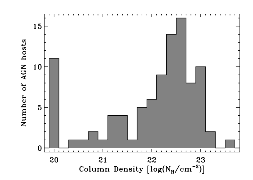
We show the distribution of column densities in Figure 1. Forty-three sources have been assigned a column density of cm, indicating minimal attenuation of the soft-band X-ray flux. Using a Kolmogorov-Smirnov (K-S) test (Fasano & Franceschini 1987), we compare the X-ray luminosity distributions and redshift distributions of the 43 AGNs having cm with that of the 316 AGNs having cm. A K-S test indicates a scaled maximum deviation () between the cumulative distributions of two data sets (such as the X-ray luminosities of the two samples). It also provides the significance level of , where and indicates that the two samples differ significantly.
The X-ray luminosity distribution of the 43 AGNs with column density cm is very similar to the distribution of the remaining AGNs (, ). The redshift distributions show a very similar discrepancy () and again a high probability of having been drawn from the same parent population (). The complete sample has a median column density cm, while the 316 AGNs that have cm exhibit a median column density of cm. The distribution that we observe between obscured AGNs (209/359 58%; cm) and unobscured AGNs (150/359 42%; cm) is consistent with established observations of the ratio between obscured and unobscured AGNs (e.g. Maiolino & Rieke 1995; Ho et al. 1997), indicating that our use of a constant power-law slope of does not adversely affect our conclusions. Of course, this sample is missing Compton thick AGNs, those that have column densities cm. Therefore, our results only apply to the Compton thin population of AGNs; however, Compton thick objects seem to be a small fraction of the AGN population (Malizia et al. 2009), and, at these redshifts, may only be associated with major mergers and interactions (Draper & Ballantyne 2010; Treister et al. 2010), and the nuclear starburst disk model would not be applicable.
XSPEC is then used once again to estimate the unabsorbed 2–10 keV X-ray fluxes, using the same spectral model and parameters and setting the source column densities to zero. We then derive the necessary k-correction for the X-ray fluxes by integrating over a power-law spectrum, which results in the following k-correction:
| (1) |
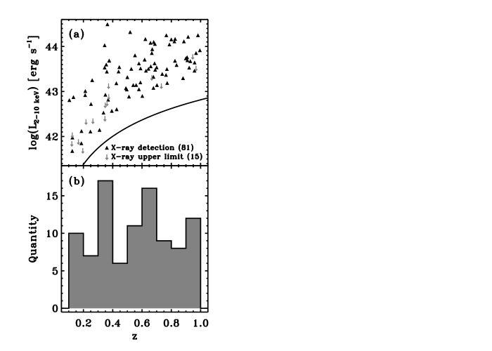
where , and we again use . Using the k-corrected, unabsorbed flux and the luminosity distance of each individual source, we finally calculate the intrinsic, rest-frame 2–10 keV luminosities. All of the unabsorbed fluxes are less than a factor of two greater than the corresponding absorbed fluxes, with a median correction factor of 1.01. Therefore, the correction for absorption does not lead to a large difference between the observed and the intrinsic X-ray luminosities. Panel (a) of Figure 2 shows the intrinsic 2–10 keV X-ray luminosities of our AGN sample, as a function of redshift. The black curve indicates the hard-band flux sensitivity limit for the survey (see table 2 from Cappelluti et al. 2009), and the gray arrows indicate the 108 X-ray sources (30% of our AGN sample) that do not have significant hard-band detections. The X-ray luminosities for these sources are derived from absorption-corrected upper limits to the hard-band X-ray fluxes (Brusa et al. 2010). The redshift distribution, peaking at and , is shown in panel (b) of Figure 2, and is very similar to the one found by Strazzullo et al. (2010) for faint radio sources with flux densities between 16 and 30 Jy. Thus, these X-ray selected AGN seem to be distributed in redshift in a similar manner to faint radio sources.
2.4 Radio observations
Radio observations of the full 2 deg2 COSMOS field, at 1.4 GHz (21 cm), comprise the VLA-COSMOS Large Project (Schinnerer et al. 2004, 2007; Bondi et al. 2008). Approximately 3600 sources have been detected at a minimum 4.5 detection significance, and the sensitivity of the observations reaches 11 Jy/beam.
We search for radio counterparts to our initial sample of 481 X-ray selected AGNs using the coordinates provided in the X-ray and radio catalogs. Searching within a circle of radius 2″ centered on each X-ray source, we find radio counterparts to 120 of the AGNs with redshifts (25%; 120/481). The most distant radio counterpart identified using this search radius is centered 1.38″ from the center of the X-ray source. Park et al. (2008) used a less conservative search radius of 2.5″ to match X-ray sources to IR sources. If instead we use the search radius used by Park et al., one of the X-ray sources has two potential radio matches, at distances of 2.48″ and 0.06″. In such a case, we would select the nearer source as the match. A brief analysis of the properties of these radio-detected AGNs is presented in Appendix A.
The radio images and fluxes of all remaining 361 AGNs are then visually examined. We do not find any that are located near known radio sources. The radio flux density measurements identify an additional two X-ray selected AGNs as possible radio sources. A visual inspection of the radio images suggests that both AGNs may be associated with true radio sources and are excluded from our sample. Thus, we arrive at 359 radio-undetected X-ray selected AGNs at .
2.5 Mid-infrared observations
Although not used for source selection, it is interesting to consider the mid-IR properties of our AGN sample. Sanders et al. (2007) describe S-COSMOS, the mid- to far-IR survey of the COSMOS field, undertaken with the Spitzer Space Telescope (Spitzer). The entire field was observed at wavelengths from 3.6 m to 160 m. Brusa et al. (2010) identified the 24-m counterparts of the COSMOS X-ray sources, using a mid-IR catalog presented by Le Floc’h et al. (2009). Eighty-four percent (301/359) of our AGNs have identified 24-m counterparts, indicating that star formation is likely occurring in these galaxies. In principle, the 24 m flux densities could be used to directly estimate the SFRs of these galaxies (e.g., Rieke et al. 2009). However, the presence of a luminous AGN will also cause mid-IR emission due to dust exposed to the AGN. The AGN contribution to the 24 m flux density will be difficult to estimate as it strongly depends on the geometrical and physical properties of the dust in the nuclear environment (e.g., Nenkova et al. 2008; Hatziminaoglou et al. 2009).
The column density distributions of the 24 m-detected and undetected AGNs are shown in Figure 3, where the solid gray histogram represents the 24 m-undetected systems (58 AGNs) and the open histogram represents the 301 AGNs that are detected at 24 m. We find a low probability () that these are drawn from the same population and a maximum deviation between the distributions of . X-ray luminosities (Figure 4 (a)) show a similar deviation () between the 24 m-detected and undetected samples and a slightly larger probability of having been drawn from the same population (). Figure 4 (a) reveals a relative lack of 24 m-undetected AGNs at the lowest redshifts of our sample (). Statistically, however, the redshifts shown in panel (b) of Figure 4 are very similar, with a 97% probability of coming from the same parent population; the maximum deviation is correspondingly low (). In summary, we find that the 24 m-detected and undetected samples represent different sub-populations within the AGN population. As they seem to be a different population, the 24 m-undetected AGNs are treated separately in the radio-stacking exercise.
3 Analysis and Results
3.1 AGN sub-samples
We split our AGN sample into several sub-samples based on various combinations of the following: redshift, detection or non-detection of 24 m flux, neutral hydrogen column density, and X-ray luminosity. All samples are first separated by detection or non-detection of 24 m flux (see Section 2.5) and then by nuclear obscuration, using a column density cm, where, following the typical convention, objects are considered obscured if they are observed through a cm. The samples are then split by redshift and/or X-ray luminosity. After trying a variety of sample sizes and grouping strategies, we conclude that samples containing 55-70 galaxies are best suited for the current work and that comparing samples of similar size greatly facilitates interpretation of our results.
Table 2 lists the criteria used to create our sub-samples. The first column provides the ID of each sample, matching references to specific samples throughout the rest of this paper. The second column indicates the number of galaxies in each sample. Columns (3)-(5) list the minimum, maximum, and median redshifts of the samples, and columns (6)-(8) list the minimum, maximum, and median X-ray luminosities. We only experiment with a few samples of the 24 m-undetected AGN host galaxies, because, as seen below, the stacked radio images do not result in a positive detection.
3.2 AGN contribution to the radio flux density
Even though our sample consists of radio undetected AGNs, that does not imply a complete lack of radio emission from the accreting black hole. As we are searching for radio emission from star formation in these AGNs, we need to correct for the AGN contribution to whatever faint radio flux density exists. Based entirely on observations of local radio quiet AGNs (Terashima & Wilson 2003), Ballantyne (2009) used the following relationship to estimate the rest-frame 5 GHz luminosity from the known X-ray luminosity:
| (2) |
where (note that there is a typographical error in the Ballantyne [2009] definition of ). The 1.4 GHz luminosity is then calculated assuming a spectral index of , where . Finally, the conversion from luminosity to flux density is
| (3) |
where is the observed 1.4 GHz flux density in units of W m-2 Hz-1, is the rest-frame 1.4 GHz luminosity in units of W Hz-1, and is the luminosity distance in meters. For our sample, the median redshift is , and the median predicted 1.4 GHz flux density is Jy. As there is a wide dispersion in the radio spectra of AGNs, we checked how our results depend on the value of . A spectral index decreases the median predicted flux density to Jy, and a steeper spectrum () increases the predicted flux density to Jy. All three values are well below the flux density limit of the COSMOS radio survey (see Table 1)222For comparison, the correlation between radio luminosities and X-ray luminosities described by Panessa et al. (2007) for a sample of nearby low luminosity Seyfert galaxies predicts a median 1.4 GHz flux density of Jy. This large value is due to the fact that low luminosity AGNs tend to be more luminous at radio frequencies (e.g., Ho & Ulvestad 2001; Nagar et al. 2002) than higher luminosity Seyferts (as parameterized in Eq. 2). Thus, the correlation based on work by Terashima & Wilson (2003) best represents the AGN contribution to the radio emission for our sample of AGNs..
To remove the estimated AGN contribution to the radio flux density for each source, we first create a radio PSF by stacking a sample of COSMOS galaxies from the COSMOS photometry catalog (Capak et al. 2007). We select galaxies that have photometric redshifts (to match our AGN sample), band magnitudes , and uncertainties on the band measurements . Galaxies outside the radio-imaged region are excluded, as are any sources flagged as having questionable photometry. We then stack the 23,941 galaxies that meet these criteria, and the resulting image is our radio PSF.
For each AGN in our sample, we scale the PSF so that a measurement of its integrated flux density matches the integrated flux density estimated from the X-ray luminosity of the AGN. We then subtract the scaled PSF image from its corresponding AGN radio image, and the residual image represents the contribution to the observed radio emission from star formation alone. It is these residual images that are then stacked using the samples listed in Table 2. If the AGN dominates any faint observed radio emission, then the stack will reveal no additional radio flux associated with star formation. However, if one of the AGN sub-populations is experiencing star formation, the integrated flux and detection significance for the residual stack may reveal this.
3.3 Stacking procedure
Two methods are commonly used to average together the input images to a stack, and some authors use both methods and then compare the results. The first of the two methods is a mean or a noise-weighted mean of the images (e.g., de Vries et al. 2007; Ivison et al. 2007; White et al. 2007). This method is preferred for a population that exhibits a flux distribution (radio flux density, in this case) that is approximately Gaussian. For samples that are likely to have non-Gaussian flux distributions, such as our sample of AGNs, a median or a clipped mean is often used (Wals et al. 2005; Boyle et al. 2007; de Vries et al. 2007; White et al. 2007; Carilli et al. 2008; Hodge et al. 2008, Dunne et al. 2009). Karim et al. (2011) present a detailed explanation of the statistics associated with both stacking methods. Because there is no obvious flux below which the remaining fluxes in our samples follow a Gaussian distribution, we combine the individual residual radio images for each sample using a median stacking method.
Each of the stacked images are then analyzed using the AIPS task
JMFIT and fluxes are measured with a single two-dimensional
elliptical Gaussian that is fit to a 12 pixel x 12 pixel region
(4.2″ x 4.2″). This analysis region is
centered at the image center, which corresponds to the locations of
the X-ray sources.
In order to estimate measurement uncertainties, the AIPS task
JMFIT calculates the root-mean-square of each image within a
specified radius of the center of the analysis region; we use a
15-pixel radius. The task runs for up to 1000 iterations, stopping as
soon as it converges on a solution. The output includes the peak and
integrated radio flux densities, along with estimated uncertainties on each
measurement. We define the signal-to-noise ratio (S/N) of each
measurement as the peak flux density divided by its corresponding
uncertainty.
3.4 Stacking results
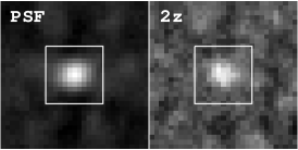
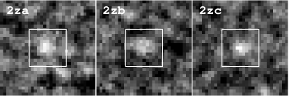
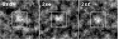
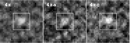
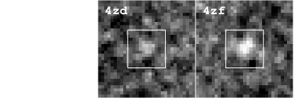
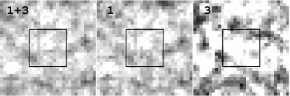
Figure 5 shows the 15 stacked residual radio images, as
listed in Table 2; the PSF is also shown. We
indicate on the figure the 12 pixel x 12 pixel regions that are used
by the AIPS task JMFIT to measure the peak and integrated flux
densities of the stacked images. The first 12 samples feature a
visually identifiable radio source, while the last three images
represent the three samples that are not detected at 24 m and
show an apparent lack of radio flux. The colors of the latter three
images are inverted to more clearly show the effect of subtracting the
PSF.
Table 3 provides flux densities, detection significances, and SFRs for the residual radio image stacks. The first column lists the sample ID, matching those provided in Table 2. Column (2) lists the integrated flux densities of the stacked samples, together with the associated uncertainties. In column (3), we list the S/N of each stacked sub-sample. Star formation rates calculated following equation (6) of Bell (2003) are provided in column (4) for the samples having non-negative integrated flux densities. The SFR uncertainties are based on the uncertainties measured with the integrated flux densities.
As already suggested by Figure 5, the first 12 samples show evidence of radio emission, with the S/N ranging from 3.1 to 7.6. Note that the two samples with the highest S/N – 2z and 4z – contain the most AGNs; the remainder of the “2” and “4” series are sub-sets of the 2z and 4z samples, respectively. When making catalogs of radio sources, detections with a high significance are required to ensure the exclusion of false detections (e.g., Richards 2000; Biggs & Ivison 2006; Ivison et al. 2007; Schinnerer et al. 2007; Morrison et al. 2010). However, when using the stacking method, we know the locations of the potential sources, which allows for less strict criteria for a positive detection. All of our 24 m-detected samples are detected with S/N , indicating a significant radio detection in the stacked image.
In contrast, the 24 m-undetected samples show no positive radio emission, independent of sample size. The integrated flux densities are negative, but from zero. These negative flux densities might be evidence that the AGN correction that is subtracted from each image is too large. To test this possibility these three radio stacks were recalculated with no AGN correction. The resulting stacked images have a negative integrated flux density for the unobscured sample (“3”), and positive flux densities for the complete (“1+3”; ) and obscured (“1”; ) samples. The unobscured sub-sample (“3”) only has 14 objects and therefore the null result for this group of AGNs is likely directly related to the relatively small number of AGNs that comprise the stack. The complete sample and the obscured sub-sample do result in weak positive radio detections, yet these disappear if the AGN correction is performed prior to stacking (Table 3). The estimated AGN radio flux density depends only on X-ray luminosity (Eq. 2), so the mean correction for the obscured 24 m-undetected sample with will be very similar to the one for the “2ze” sample (with ), and the mean correction for the complete sample (with ) will be similar to the one for the “2zd” sample (with ). Both the “2ze” and the “2zd” samples have significant positive detections in the residual stacks with similar numbers of objects as the 24 m-undetected stacks. If the predicted AGN radio flux density was overestimated than it would have a comparable effect in all of these samples. Therefore, we can conclude that the objects in the 24 m-detected samples must, on average, be stronger radio emitters than the 24 m-undetected AGNs, with the additional flux arising from star formation. However, as described in Sect. 2.5, the 24 m-undetected AGNs seem to arise from a different population than the ones that are detected at 24 m. It is thus possible that the negative flux densities found in the stacked images of the 24 m-undetected AGNs may indicate that this population of AGNs produces weaker nuclear radio fluxes than the 24 m-detected AGNs, and our AGN correction (Eq. 2) is an overestimate for this population.
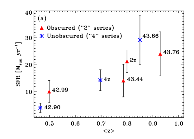
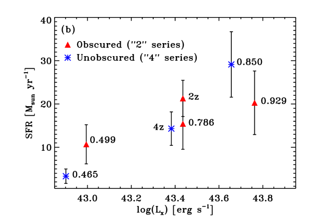
In Figure 6, we show the SFRs of our samples as a function of redshift (upper panel) and X-ray luminosity (lower panel). The full obscured and unobscured samples are labeled with “2z” and “4z”, respectively. In the upper panel the other symbols represent the samples that depend on redshift and are labeled with their median X-ray luminosities, while the lower panel features the samples dependent on luminosity and are labeled with their median redshifts. The estimated SFRs are in the range yr, which are exactly the rates predicted by nuclear starburst disk models (Ballantyne 2008). Unsurprisingly, we observe an increase in the SFR with redshift, consistent with the peak of star formation and supermassive black hole growth observed at (e.g., Le Floc’h et al. 2005). As there is a correlation between redshift and luminosity (Figure 2), this correlation also appears in the luminosity panel. Comparing the SFRs of the three higher redshift samples that have similar median luminosities shows that both the obscured and the unobscured AGNs have similar levels of star formation.
Our choice of a spectral index for the AGN radio emission also affects the SFR estimates. We recalculate the SFRs for the 12 samples that have 24 m detections using spectral indices of and . In both cases, the resulting star formation rates are typically lower than those determined for , but the deviations from the SFRs reported in Table 3 are less than the uncertainties derived from the integrated radio flux density measurements.
4 Discussion and Conclusions
The AGN population at is predominately comprised of obscured objects with Seyfert luminosities (e.g., Ueda et al. 2003), yet the evolutionary state of these galaxies is largely unknown. At these luminosities, it is possible that a significant number of AGNs are not fueled by the violent mergers of massive galaxies, but are undergoing a more leisurely mode of galaxy assembly (e.g., Ballantyne et al. 2006; Hasinger 2008; Lutz et al. 2010). In this case, gas will be slowly fed into the nuclear regions where significant star formation will occur en route to the black hole accretion disk. It is possible that such a nuclear starburst could provide a location for the X-ray obscuration seen in most of these AGNs (Ballantyne 2008). In this paper, we searched for evidence for this star formation process by considering the faint radio emission from 481 X-ray selected AGNs in the COSMOS field. The X-ray properties (i.e., obscuration and luminosity) of this sample were consistent with the AGNs that dominate the X-ray background and can be fueled and obscured by nuclear starbursts.
As expected from the nuclear starburst model, well over half of these AGNs (359) were undetected in the VLA 1.4 GHz COSMOS survey, so radio stacking techniques were employed to search for faint radio emission in samples that were selected based on redshift, X-ray luminosity, and obscuration. Objects with 24 m detections (301 out of the 359) were considered separately from those which were undetected at 24 m. An estimate for the nuclear AGN radio flux density was subtracted from each image prior to stacking. For AGNs with a 24 m detection, the stacked images had a positive radio source corresponding to SFRs of yr, consistent with the predictions of a nuclear starburst (Ballantyne 2008). As expected, the SFRs increased with the redshift of the samples, but there was no clear dependence on either luminosity or X-ray obscuration, consistent with the unified model of AGNs and the starburst disk model.
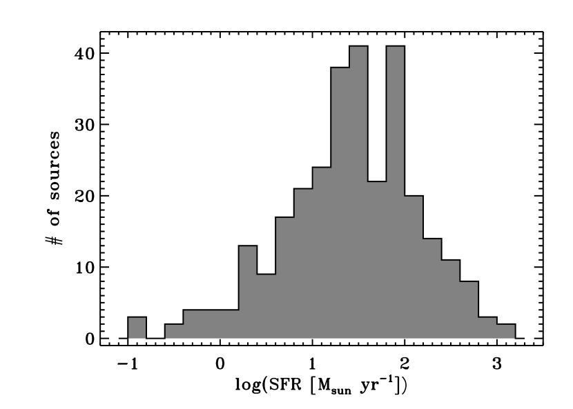
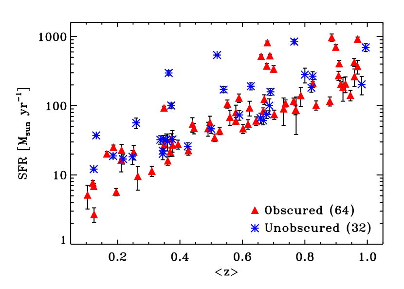
The radio stacking was pursued because it was predicted to be a potentially cleaner test for the presence of star formation than the mid-infrared. It is interesting, therefore, to compare the SFRs obtained from the stacking exercise to the ones calculated directly from the 24 m flux densities. Brand et al. (2006) estimates that objects with mJy are dominated by starbursts. Using this criterion, 95% (287/301) of the 24 m sources matched to our AGNs appear to be dominated by star formation rather than the AGN, although the AGN will still contribute an unknown amount of flux to many of these 24 m sources. Figure 7 plots the distribution of SFRs calculated directly from the 24 m flux density (Reike et al. 2009) for all 301 AGN host galaxies. The median SFR is 29 yr-1 which is the same as the maximum SFR found in the radio stacks. This result implies that the AGN contributes a non-negligible fraction of the 24 m flux in at least 50% of these galaxies.
The SFRs derived from the radio stacks are consistent with measurements of both active and inactive host galaxies at these redshifts. Mullaney et al. (2011) recently studied a sample of X-ray selected AGNs at redshifts , combining deep, high-resolution Herschel observations at 100 m and 160 m with spectral energy distribution templates (Chary & Elbaz 2001) to estimate the total IR luminosities and the SFRs. For the subset of their AGNs at the redshifts and X-ray luminosities of the current study, Mullaney et al. (2011) found SFRs that are very similar to the SFRs reported herein. Similarly, Noeske et al. (2007) measured SFRs with optical/UV/IR techniques of massive inactive galaxies in the Extended Groth Strip at redshifts . In particular, their figure 1 shows the increase in the SFR with redshift, and our results fall roughly near the median SFR for similar redshift and stellar mass (Capak et al. 2007) bins. This result suggests that the AGN radio correction employed above is at the appropriate level, and that these AGN host galaxies are forming stars at rates similar to both active and inactive galaxies of the same size and age. This is further evidence that host galaxies of the Compton thin Seyferts that dominate the XRB are not in the throes of a massive merger.
Interestingly, none of the 24 m-undetected samples produce a positive radio detection in the stacked image, which indicates that, on average, these are very weak star-forming galaxies. To check for possible faint star formation among the 24 m-undetected sources we make use of the observed and colors. At the redshifts of our sample () these colors approximately correspond to the rest-frame colors used by Williams et al. (2009) to separate faint or dusty galaxies from quiescent galaxies. Fifty of the 58 AGNs not detected at 24 m have colors suggestive of faint star formation []. If we add these AGNs to the samples of 24 m-detected AGNs, and repeat the radio stacking measurements, the resulting SFRs are consistent with the SFRs presented in Sect. 3.4, which are based on the simple separation between detection or non-detection at 24 m. Thus, the majority do seem to have very little ongoing star formation, despite hosting a reasonably luminous AGN. Recall that these galaxies also seem to arise from a different population than the 24 m-detected objects (see Section 2.5), with a larger fraction of obscured, low-luminosity AGNs. The X-ray obscuration must arise from either a dust poor medium, or, perhaps more likely, from galactic scale obscuration (e.g., Rigby et al. 2006). These AGNs are apparently residing in relatively inactive galaxies, and thus may be in an interesting evolutionary stage. A morphological and spectral energy distribution study of these 24 m-undetected AGNs is necessary to fully understand the nature of these objects.
In conclusion, the radio stacking results presented here, combined with the SFRs found in the radio-detected AGNs (see Appendix A), show that SFRs yr-1 are present in the host galaxies of Compton thin X-ray selected AGNs at . The association of 24 m detections with low levels of star formation is consistent with models of nuclear starburst disks as sources for AGN fueling and obscuration in Seyfert galaxies. However, a significant improvement in the sensitivity and resolution of radio images for galaxies is needed to reliably determine the location of the potential star formation that has been detected. It is possible that future studies of radio spectral index and fractional polarization measurements may be useful discriminants between AGN-related and SF-related radio emission in these galaxies. Other future work will involve examining the Herschel photometry of the samples, as well as a thorough investigation of the properties of the 58 24 m-undetected AGNs. For the present time, we can say with certainty that Compton thin, X-ray selected AGN host galaxies at are emitting faint radio fluxes, but it is not yet clear if the emission originates in the nuclear regions or instead in the bulge or disk.
Appendix A Radio-detected AGNs
In Section 2.4, we found that 120 of the 481 X-ray selected AGNs with redshifts are identified as radio sources. The radio emission of some fraction of these is expected to be dominated by the AGN (often referred to as “radio-loud”), while star formation is expected to contribute a significant portion of the radio emission from the remaining radio-detected AGNs (often known as “radio-quiet”). Terashima & Wilson (2003) found that represents an approximate division between radio-loud [] and radio-quiet [] AGNs. Again assuming for the AGN radio spectrum, we identify 24 radio-loud AGNs, which is 20% (24/120) of the radio-detected sample and only 5% (24/481) of the full X-ray selected AGN sample. If we instead use , we identify 31 radio-loud AGNs (26% of the radio-detected sample), and if we use , 21 (18%) of the radio-detected sources are identified as radio-loud. For the remainder of this Appendix, we turn our focus to the 96 radio-quiet AGNs identified using and compare them to the radio-undetected AGN population described in Section 2.3.
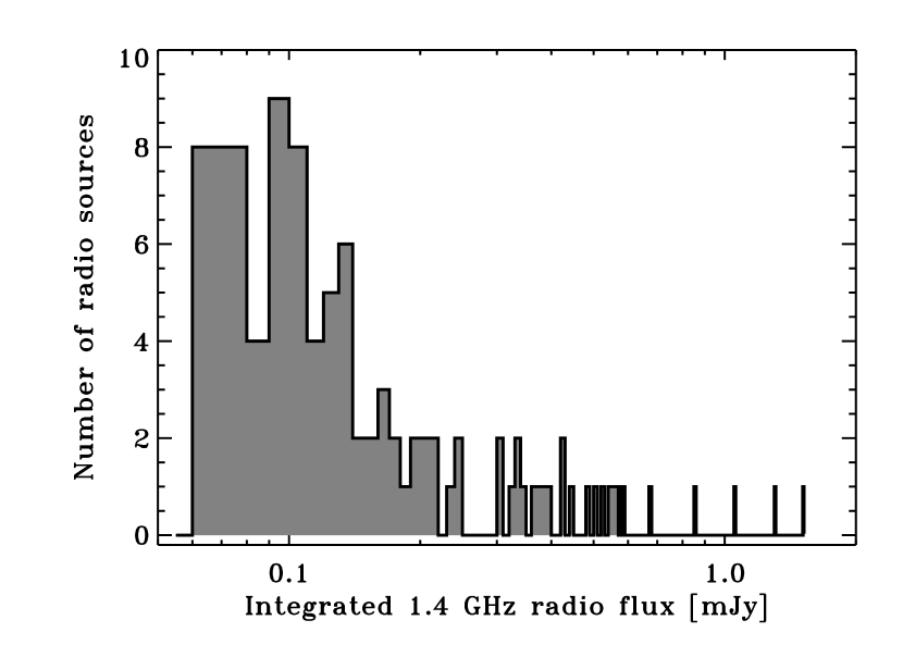
The distribution of radio flux densities for the radio-quiet AGNs is shown in Figure A1. These systems have a median radio flux density of mJy. Figure A2 shows the column density distribution of the 96 radio-quiet AGNs, which can be compared to Figure 1. The median column density is cm, and a K-S test between the column densities of the radio-quiet AGNs and the radio-undetected AGNs confirms the apparent similarity between Figures 1 and A2, with a 23% probability of having been drawn from the same parent population and a low maximum deviation (). The X-ray luminosities and redshift distribution of the radio-quiet AGNs are shown in Figure A3 (compare to Figure 2). The radio-quiet AGNs exhibit a broader X-ray luminosity distribution than the radio-undetected AGNs, especially at redshifts . Statistically, however, the X-ray luminosity distributions are not very different (, ). In contrast, panel (b) of Figure A3 shows that the radio-detected AGNs have a much flatter redshift distribution than do the radio undetected AGNs. A K-S test confirms this difference; the maximum deviation is and the probability that the distributions represent the same sample is quite low (). Finally, of the radio-quiet AGNs are also 24 m-detected.
Eqs. 2–3 are again used to estimate and remove the AGN contribution to the measured radio flux density. As before, we use a spectral index , but we also check the effect of varying the spectral index. The median predicted 1.4 GHz flux density for the radio-quiet sources is Jy when we use . A flatter spectrum () results in a lower median predicted flux density (Jy). Using a steeper spectrum () increases the predicted flux density to Jy. Figure A4 plots the mid-IR to residual radio flux density ratio for those AGNs detected at 24 m. The logarithm of the median flux ratio is , which strongly supports the interpretation that the residual radio emission originates from star formation (Seymour et al. 2008).
Figure A5 shows the SFRs computed from the residual radio flux densities as a function of redshift for the obscured and unobscured radio-quiet AGNs, with median rates of 77 yr-1 and 42 yr-1, respectively, and an overall median rate of 65 yr-1. Increasing the spectral index to increases the median SFRs to 72 yr-1, and decreasing it to similarly decreases the median star formation rate to 50 yr-1.
More than 90% of the radio-quiet AGN host galaxies are undergoing star formation at rates in excess of 10 yr-1, and 35% are experiencing SFRs exceeding 100 yr-1. These values are again largely consistent with those predicted by nuclear starburst disks (Ballantyne 2008), although with a larger fraction of high SFRs ( yr-1). This fact will be largely due to the increase in detectable SFRs with in a flux limited survey. Combining this result with the stacking analysis from Section 3.4, indicates that the majority of 24 m-detected, X-ray selected AGNs at are accompanied by star formation at levels of yr-1.
References
- (1) Antonucci, R. 1993, ARA&A, 31, 473
- (2) Adelman-McCarthy, J. K., et al. 2006, ApJS, 162, 38
- (3) Ballantyne, D. R., Everett, J. E., & Murray, N. 2006, ApJ, 639, 740
- (4) Ballantyne, D. R. 2008, ApJ, 685, 787
- (5) —. 2009, ApJ, 698, 1033
- (6) Bauer, F. E., Alexander, D. M., Brandt, W. N., Hornschemeier, A. E., Vignali, C., Gamire, G. P., & Schneider, D. P. 2002, AJ, 124, 1839
- (7) Bell, E. F. 2003, ApJ, 586, 794
- (8) Biggs, A. D., & Ivison, R. J. 2006, MNRAS, 371, 963
- (9) Bondi, M., Ciliegi, P., Schinnerer, E., Smolić, V., Jahnke, K., Carilli, C., & Zamorani, G. 2008, ApJ, 681, 1129
- (10) Boyle, B. J., Cornwell, T. J., Middelberg, E., Norris, R. P., Appleton, P. N., & Smail, I. 2007, MNRAS, 376, 1182
- (11) Brand, K., et al. 2006, ApJ, 644, 143
- (12) Brusa, M., et al. 2010, ApJ, 716, 348
- (13) Capak, P., et al. 2007, ApJS, 172, 116
- (14) Cappelluti, N., et al. 2009, A&A, 497, 635
- (15) Carilli, C. L., et al. 2008, ApJ, 689, 883
- (16) Chang, P., Quataert, E., & Murray, N. 2007, ApJ, 662, 94
- (17) Chary, R., & Elbaz, D. 2001, ApJ, 556, 562
- (18) de Vries, W. H., Hodge, J. A., Becker, R. H., White, R. L., & Helfand, D. J. 2007, AJ, 134, 457
- (19) Draper, A. R., & Ballantyne, D. R. 2010, ApJ, 715, L99
- (20) Dunne, L., et al. 2009, MNRAS, 394, 3
- (21) Elvis, M., et al. 2009, ApJS, 184, 158
- (22) Elitzur, M., & Shlosman, I. 2006, ApJ, 648, L101
- (23) Fabian, A. C., Barcons, X., Almaini, O., & Iwasawa, K. 1998, MNRAS, 297, L11
- (24) Fasano, G., & Franceschini, A. 1987, MNRAS, 225, 155
- (25) Gilli, R., Comastri, A., & Hasinger, G. 2007, A&A, 463, 79
- (26) Hasinger, G. 2008, A&A, 490, 905
- (27) Hasinger, G., et al. 2007, ApJS, 172, 29
- (28) Hatziminaoglou, E., Fritz, J., & Jarrett, T. H., 2009, MNRAS, 399, 1206
- (29) Ho, L. C., Filippenko, A. V., & Sargent, W. L. W. 1997, ApJ, 487, 568
- (30) Ho, L. C., & Ulvestad, J. S. 2001, ApJS, 133, 77
- (31) Hodge, J. A., Becker, R. H., White, R. L., & de Vries, W. H. 2008, AJ, 136, 1097
- (32) Ibar, E., & Lira, P., 2007, A&A, 466, 531
- (33) Ivison, R. J., et al. 2007, ApJ, 660, L77
- (34) Karim, A., et al. 2011, ApJ, 730, 61
- (35) Kauffmann, G., et al. 2003, MNRAS, 346, 1055
- (36) Knigl, A., & Kartje, J. F. 1994, ApJ, 434, 446
- (37) Krolik, J. H. 2007, ApJ, 661, 52
- (38) Krolik, J. H., & Begelman, M. C. 1988, ApJ, 329, 702
- (39) Le Floc’h, E., et al. 2005, ApJ, 632, 169
- (40) —. 2009, ApJ, 703, 222
- (41) Lilly, S. J., et al. 2007, ApJS, 172, 70
- (42) —. 2008, Messenger, 134, 35
- (43) —. 2009, ApJS, 184, 218
- (44) Lutz, D., et al. 2010, ApJ, 712, 1287
- (45) Mainieri, V., et al. 2007, ApJS, 172, 368
- (46) Maiolino, R., & Rieke, G. H. 1995, ApJ, 454, 95
- (47) Malizia, A., Stephen, J. B., Bassani, L., Bird, A. J., Panessa, F., & Ubertini, P. 2009, MNRAS, 399, 944
- (48) Morrison, G. E., Owen, F. N., Dickinson, M., Ivison, R. J., & Ibar, E. 2010, ApJS, 188, 178
- (49) Mullaney, J. R., et al. 2011, MNRAS, submitted, arXiv:1106.4284v2
- (50) Nagar, N. M., Falcke, H., Wilson, A. S., & Ulvestad, J. S. 2002, A&A, 392, 53
- (51) Nandra, K., & Pounds, K. A. 1994, MNRAS, 268, 405
- (52) Nenkova, M., Sirocky, M. M., Ivezić, Ž., & Elitzur, M. 2008a, ApJ, 685, 147
- (53) Nenkova, M., Sirocky, M. M., Nikutta, R., Ivezić, Ž., & Elitzur, M. 2008b, ApJ, 685, 160
- (54) Noeske, K. G., et al. 2007, ApJ, 660, L43
- (55) Panessa, F., Barcons, X., Bassani, L., Cappi, M., Carrera, F. J., Ho, L. C., & Pellegrini, S. 2007, A&A, 467, 519
- (56) Park, S. Q., et al. 2008, ApJ, 678, 744
- (57) Pier, E. A., & Krolik, J. H. 1992, ApJ, 401, 99
- (58) Prescott, M. K. M., Impey, C. D., Cool, R. J., & Scoville, N. Z. 2006, ApJ, 644, 100
- (59) Richards, E. A. 2000, ApJ, 533, 611
- (60) Rieke G. H., Alonso-Herrero A., Weiner B. J., Pérez-González P. G., Blaylock M., Donley J. L., & Marcillac D. 2009, ApJ, 692, 556
- (61) Rigby, J. R., Rieke, G. H., Donley, J. L., Alonso-Herrero, A., & Pérez-González, P. G. 2006, ApJ, 645, 115
- (62) Sanders, D. B., et al. 2007, ApJS, 172, 86
- (63) Salvato, M., et al. 2009, ApJ, 690, 1250
- (64) Schinnerer, E., et al. 2004, AJ, 128, 1974
- (65) —. 2007, ApJS, 172, 46
- (66) Scoville, N., et al. 2007, ApJS, 172, 1
- (67) Seymour, N., Dwelly, T., Moss, D., McHardy, I., Zoghbi, A., Rieke, G., Page, M., Hopkins, A., & Loaring, N. 2008, MNRAS, 386, 1695
- (68) Shi, J., & Krolik, J. H. 2008, ApJ, 679, 1018
- (69) Strazzullo, V., Pannella, M., Owen, F. N., Bender, R., Morrison, G. E., Wang, W.-H., & Shupe, D. L. 2010, ApJ, 714, 1305
- (70) Terashima, Y., & Wilson, A. S. 2003, ApJ, 583, 145
- (71) Thompson, T. A., Quataert, E., & Murray, N. 2005, ApJ, 630, 167
- (72) Treister, E., Natarajan, P., Sanders, D. B., Urry, C. M., Schawinski, K., & Kartaltepe, J. 2010, Science, 328, 600
- (73) Trump, J. R., et al. 2007, ApJS, 172, 383
- (74) —. 2009, ApJ, 1195
- (75) Ueda, Y., Akiyama, M., Ohta, K., & Miyaji, T. 2003, ApJ, 598, 886
- (76) Wada, K., & Norman, C. 2002, ApJ, 566, L21
- (77) Wals, M., Boyle, B. J., Croom, S. M., Miller, L., Smith, R., Shanks, T., & Outram, P. 2005, MNRAS, 360, 453
- (78) White, R. L., Helfand, D. J., Becker, R. H., Glikman, E., & de Vries, W. 2007, ApJ, 654, 99
- (79) Williams, R. J., Quadri, R. F., Franx, M., van Dokkum, P., & Labbé, I. 2009, ApJ, 691, 1879
- (80)
- (81)
| Telescope | Band | Sensitivity Limits | References | |
|---|---|---|---|---|
| XMM-Newton | Hard band | 3.1 Å (4 keV) | erg s-1 cm-2 | (1) |
| Soft band | 12.4 Å (1 keV) | erg s-1 cm-2 | (1) | |
| Very Large Array | 1.4 GHz | 21 cm | 11 Jy/beam | (2) |
References. — (1) Hasinger et al. 2007, Cappelluti et al. 2009. (2) Schinnerer et al. 2007, Bondi et al. 2008.
| Sample | # | zmin | zmax | cm | ||||
|---|---|---|---|---|---|---|---|---|
| (1) | (2) | (3) | (4) | (5) | (6) | (7) | (8) | (9) |
| 24 m-detected, cm 22 | ||||||||
| 2z | 165 | 0.000 | 1.000 | 0.800 | 41.50 | 44.50 | 43.44 | 22.52 |
| 2za | 54 | 0.000 | 0.678 | 0.499 | 41.50 | 44.50 | 42.98 | 22.37 |
| 2zb | 55 | 0.678 | 0.859 | 0.786 | 41.50 | 44.50 | 43.49 | 22.53 |
| 2zc | 56 | 0.859 | 1.000 | 0.929 | 41.50 | 44.50 | 43.66 | 22.58 |
| 2zd | 55 | 0.000 | 1.000 | 0.518 | 41.50 | 43.27 | 42.99 | 22.33 |
| 2ze | 55 | 0.000 | 1.000 | 0.830 | 43.27 | 43.59 | 43.44 | 22.52 |
| 2zf | 55 | 0.000 | 1.000 | 0.884 | 43.59 | 44.50 | 43.76 | 22.66 |
| 24 m-detected, cm 22 | ||||||||
| 4z | 136 | 0.000 | 1.000 | 0.697 | 41.50 | 44.50 | 43.38 | 21.39 |
| 4za | 69 | 0.000 | 0.700 | 0.465 | 41.50 | 44.50 | 42.90 | 21.39 |
| 4zc | 67 | 0.700 | 1.000 | 0.850 | 41.50 | 44.50 | 43.59 | 21.38 |
| 4zd | 67 | 0.000 | 1.000 | 0.466 | 41.50 | 43.38 | 42.90 | 21.46 |
| 4zf | 69 | 0.000 | 1.000 | 0.820 | 43.38 | 44.55 | 43.59 | 21.19 |
| 24 m-undetected | ||||||||
| 1+3a | 58 | 0.000 | 1.000 | 0.767 | 41.50 | 44.50 | 43.19 | 22.44 |
| 1b | 44 | 0.000 | 1.000 | 0.780 | 41.50 | 44.50 | 43.33 | 22.52 |
| 3c | 14 | 0.000 | 1.000 | 0.684 | 41.50 | 44.50 | 42.96 | 21.18 |
Note. — Column (1): sample ID, which matches references to specific samples throughout the paper. Column (2): number of galaxies in each sample. Columns (3)-(5): minimum, maximum, and median redshifts. Columns (6)-(8): logarithm of the minimum, maximum, and median 2–10 keV X-ray luminosities, in units of erg s-1. Column (9): logarithm of the median column density, in units of cm-2.
| ID | Integrated flux density | S/N | SFR |
|---|---|---|---|
| (Jy) | ( yr-1) | ||
| (1) | (2) | (3) | (4) |
| 24 m-detected, cm 22 | |||
| 2z | 15.3 3.0 | 7.6 | 21 4 |
| 2za | 21.6 8.9 | 3.2 | 10 4 |
| 2zb | 10.6 4.5 | 3.7 | 14 6 |
| 2zc | 12.2 4.1 | 4.7 | 24 8 |
| 2zd | 21.0 8.9 | 3.1 | 10 5 |
| 2ze | 10.2 3.9 | 4.4 | 15 6 |
| 2zf | 11.5 4.2 | 4.3 | 20 7 |
| 24 m-detected, cm 22 | |||
| 4z | 14.1 3.8 | 5.4 | 14 4 |
| 4za | 10.2 4.3 | 3.7 | 4.1 1.7 |
| 4zc | 18.2 5.7 | 4.5 | 29 9 |
| 4zd | 8.1 4.1 | 3.3 | 3.3 1.7 |
| 4zf | 19.7 5.1 | 5.5 | 29 8 |
| 24 m-undetected | |||
| 1+3 | -34.2 19.9 | … | … |
| 1 | -20.0 10.9 | … | … |
| 3 | -39.4 18.8 | … | …
|
Note. — IDs correspond to the samples listed in Table 2.