Prandtl and Rayleigh number dependence of heat transport in high Rayleigh number thermal convection

Abstract

Results from direct numerical simulation for three-dimensional Rayleigh-Bénard convection in samples of aspect ratio $\Gamma=0.23$ and $\Gamma=0.5$ up to Rayleigh number $Ra=2\times 10^{12}$ are presented. The broad range of Prandtl numbers $0.5<Pr<10$ is considered. In contrast to some experiments, we do not see any increase in $Nu/Ra^{1/3}$, neither due to $Pr$ number effects, nor due to a constant heat flux boundary condition at the bottom plate instead of constant temperature boundary conditions. Even at these very high $Ra$, both the thermal and kinetic boundary layer thicknesses obey Prandtl-Blasius scaling.

1 Introduction

In Rayleigh-Bénard (RB) convection fluid in a box is heated from below and cooled from above (Ahlers et al. (2009c)). This system is paradigmatic for turbulent heat transfer, with many applications in atmospheric and environmental physics, astrophysics, and process technology. Its dynamics is characterized by the Rayleigh number $Ra=\beta g\Delta L^{3}/(\kappa\nu)$ and the Prandtl number $Pr=\nu/\kappa$. Here, $L$ is the height of the sample, $\beta$ is the thermal expansion coefficient, $g$ the gravitational acceleration, $\Delta$ the temperature difference between the bottom and the top of the sample, and $\nu$ and $\kappa$ the kinematic viscosity and the thermal diffusivity, respectively. Almost all experimental and numerical results on the heat transfer, indicated by the Nusselt number $Nu$, agree up to $Ra\approx 2\times 10^{11}$ (see the review of Ahlers et al. (2009c) for detailed references) and are in agreement with the description of the Grossmann-Lohse (GL) theory (Grossmann & Lohse (2000, 2001, 2002, 2004)). However, for higher $Ra$ the situation is less clear.

Figure 1: Visualization of the instantaneous temperature and temperature (left) and vertical velocity field (right) for the simulation at $Ra=2\times 10^{12}$ and $Pr=0.7$ for $\Gamma=0.5$. Red and blue indicate warm (up flowing) and cold (down flowing) fluid, respectively, in the left (right) panel. Corresponding movies can be found as supplementary material.

Most experiments for $Ra\gtrsim 2\times 10^{11}$ are performed in samples with aspect ratios $\Gamma\equiv D/L=0.5$ and $\Gamma=0.23$, where $D$ and $L$ are the diameter and height of the sample, respectively. The majority of these experiments are performed with liquid helium near its critical point (Chavanne et al. (2001); Niemela et al. (2000, 2001); Niemela & Sreenivasan (2006); Roche et al. (2001, 2002, 2010)). While Niemela et al. (2000, 2001) and Niemela & Sreenivasan (2006) found a $Nu$ increase with $Nu\varpropto Ra^{0.31}$, the experiments by Chavanne et al. (2001) and Roche et al. (2001, 2002, 2010) gave a steep $Nu$ increase with $Nu\varpropto Ra^{0.38}$. In these helium experiments the $Pr$ number increases with increasing $Ra$. Funfschilling et al. (2009) and Ahlers et al. (2009a, b) performed measurements around room temperature with high pressurized gases with nearly constant $Pr$ and do not find such a steep increase. Niemela & Sreenivasan (2010) found two $Nu\varpropto Ra^{1/3}$ branches in a $\Gamma=1$ sample. The high $Ra$ number branch is $20\%$ higher than the low $Ra$ number branch. By necessity, $Nu$ increases more steeply in the transition region. The scaling in the transition region happens to be around $Nu\varpropto Ra^{0.5}$. There are thus considerable differences in the heat transfer obtained in these different experiments in the high $Ra$ number regime. Very recently, Ahlers and coworkers (see Ahlers (2010) and addendum to Ahlers et al. (2009b)) even found two different branches in one experiments with the steepest branch going as $Nu\varpropto Ra^{0.36}$.

Figure 2: (a) $Nu$ vs $Ra$ for $\Gamma=0.5$. The green downward pointing triangles are experimental data from Niemela et al. (2000, 2001) after a reanalysis reported in Niemela & Sreenivasan (2006), the red squares are from Chavanne et al. (2001), the purple diamonds are from Funfschilling et al. (2009) and Ahlers et al. (2009a, b); Ahlers (2010). The DNS results for $Pr=0.7$ are indicated in black and are from Stevens et al. (2010b). The data point for $Ra=2\times 10^{12}$ is from this study. When the vertical error bar is not visible the error is smaller than the dot size. (b) Parameter space for the data presented in panel a. Symbols as in panel a.

Figure 3: (a) $Nu$ vs $Ra$ for $\Gamma=0.23$. The upward pointing red triangles are from Roche et al. (2010). The DNS results for $Pr=0.7$ and $Pr=2.0$ are indicated in black and blue, respectively. When the vertical error bar is not visible the error is smaller than the dot size. (b) Parameter space for the data presented in panel a. Symbols as in panel a. The black squares indicate DNS simulations presented in this paper.

There is no clear explanation for this disagreement although it has been conjectured that variations of the $Pr$ number, the use of constant temperature or a constant heat flux condition at the bottom plate, the finite conductivity of the horizontal plates and side wall, non Oberbeck-Boussinesq effects, i.e. the dependence of the fluid properties on the temperature, the existence of multiple turbulent states (Grossmann & Lohse (2011)), and even wall roughness and temperature conditions outside the sample might play a role. Since the above differences among experiments might be induced by unavoidable technicalities in the laboratory set–ups, within this context, direct numerical simulations are the only possibility to obtain neat reference data that strictly adhere to the intended theoretical problem and that could be used as guidelines to interpret the experiments: This is the main motivation for the present study.

2 Numerical procedure

We start this paper with a description of the numerical procedure that is used to investigate the influence on the heat transfer for two of the issues mentioned above. First, we discuss the effect of the $Pr$ number on the heat transport in the high $Ra$ number regime. Subsequently, we will discuss the difference between simulations performed with a constant temperature at the bottom plate with simulations with a constant heat flux at the bottom plate. We take the constant heat flux condition only at the bottom plate, because in real setups the bottom plate is in contact with a heater while the top plate is connected to a thermostatic bath. Thus, the condition of constant heat flux applies at most only to the bottom plate (Niemela et al. (2000, 2001) and Niemela & Sreenivasan (2006)). At the top plate constant temperature boundary conditions are assumed to strictly hold, i.e. perfect heat transfer to the recirculating cooling liquid. We will conclude the paper with a brief summary, discussion, and outlook to future simulations.

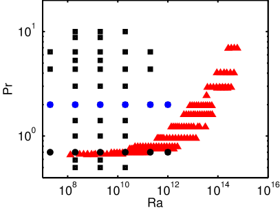
The flow is solved by numerically integrating the three-dimensional Navier-Stokes equations within the Boussinesq approximation. The numerical method is already described in Verzicco & Camussi (1997, 2003) and Verzicco & Sreenivasan (2008) and here it is sufficient to mention that the equations in cylindrical coordinates are solved by central second-order accurate finite-difference approximations in space and time. We performed simulations with constant temperature conditions at the bottom plate for $2\times 10^{7}<Ra<1\times 10^{12}$ and $0.5<Pr<10$ in an aspect ratio $\Gamma=0.23$ sample. We also present results for a simulation at $Ra=2\times 10^{12}$ at $Pr=0.7$ in a $\Gamma=0.5$ sample. In addition, we performed simulation with a constant heat flux at the bottom plate and a constant temperature at the top plate, see Verzicco & Sreenivasan (2008) for details, for $Pr=0.7$, $\Gamma=0.5$, and $2\times 10^{6}\leq Ra\leq 2\times 10^{11}$. Because in all simulations the temperature boundary conditions are precisely assigned, the surfaces are infinitely smooth, and the Boussinesq approximation is unconditionally valid, the simulations provide a clear reference case for present and future experiments.

In Stevens et al. (2010b) we investigated the resolution criteria that should be satisfied in a fully resolved DNS simulation and Shishkina et al. (2010) determined the minimal number of nodes that should be placed inside the boundary layers. The resolutions used here are based on this experience and we stress that in this study we used even better spatial resolution than we used in Stevens et al. (2010b) to be sure that the flow is fully resolved.

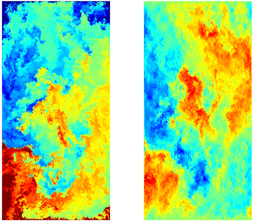
To give the reader some idea of the scale of this study we mention the resolutions that were used in the most demanding simulations, i.e., simulations that take at least 100.000 DEISA CPU hours each. For $\Gamma=0.23$ this are the simulations at $Ra=2\times 10^{11}$, which are performed on either a $641\times 185\times 1281$ (azimuthal, radial, and axial number of nodes) grid for $Pr=0.7$ and $Pr=2.0$ or on a $769\times 257\times 1537$ grid for $Pr=4.38$ and $Pr=6.4$. The simulations at $Ra=1\times 10^{12}$ are performed on a $1081\times 301\times 2049$ grid. The simulations for $Ra=2\times 10^{11}$ were run for at least $100$ dimensionless time units (defined as $L/\sqrt{\beta g\Delta L}$), while these simulations at $Ra=1\times 10^{12}$ cover about $30-40$ time units. The simulation with a constant heat flux condition at the bottom plate and constant temperature condition at the top plate in a $\Gamma=0.5$ sample with $Pr=0.7$ at $Ra=2.25\times 10^{11}$ is performed on a $1081\times 351\times 1301$ grid. The simulation at $Ra=2\times 10^{12}$ with $Pr=0.7$ in the $\Gamma=0.5$ sample has been performed on a $2701\times 671\times 2501$ grid, which makes it the largest fully bounded turbulent flow simulation ever. This simulation takes about $100.000$ vectorial CPU hours on HLRS (equivalent to $\approx 9\times 10^{6}$ DEISA CPU hours). To store one snapshot of the field ($T$, $u_{1}$,$u_{3}$, because $u_{2}$ follows from continuity) costs 160 GB in binary format. A snapshot of this flow is shown in figure 1. Movies of this simulation are included in the supplementary material.

3 Numerical results on $Nu(Ra,Pr,\Gamma)$

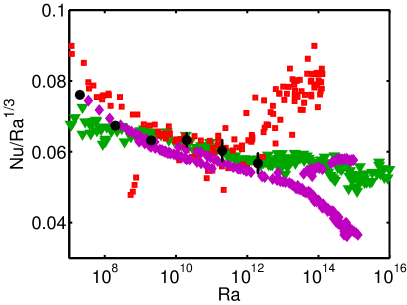
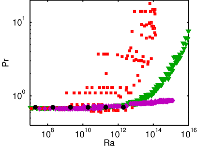
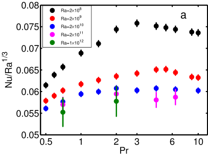
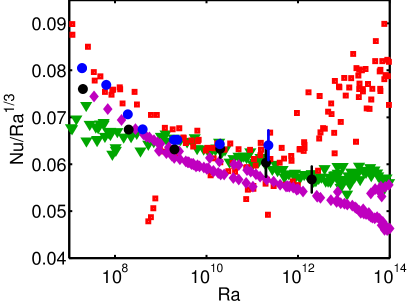
In figure 2a and figure 3 the DNS results for $Pr=0.7$ in the $\Gamma=0.23$ and $\Gamma=0.5$ samples are compared with experimental data. The result for $Ra=2\times 10^{12}$ in the $\Gamma=0.5$ sample agrees well with the experimental data of Niemela et al. (2000, 2001), Niemela & Sreenivasan (2006), Funfschilling et al. (2009), and Ahlers et al. (2009a, b), while there is a visible difference with the results of Chavanne et al. (2001). A comparison of the results for $\Gamma=0.23$ with the experimental data of Roche et al. (2010) shows that there is a good agreement for higher $Ra$ numbers, while for lower $Ra$ we obtain slightly larger $Nu$ than in those experiments. We again stress that we performed resolution checks for this $\Gamma=0.23$ case (up to $Ra=2\times 10^{10}$), and in addition considering the good agreement with the results for $\Gamma=0.5$, we exclude that our DNS results overestimate $Nu$.

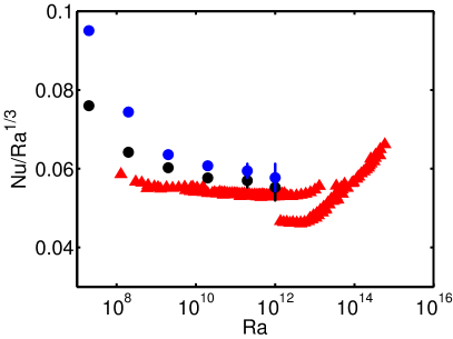
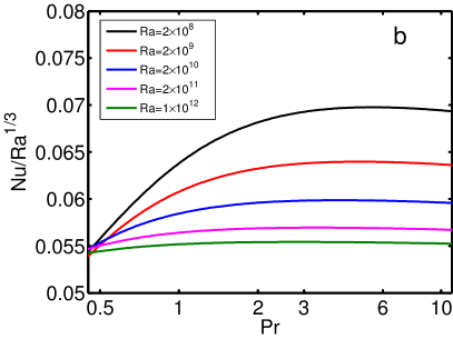
Figure 2b and 3 show that in some experiments the $Pr$ number increases with increasing $Ra$. This difference in $Pr$ is often mentioned as one of the possible causes for the observed differences in the heat transfer between the experiments. Figure 4 shows the $Nu$ number as function of $Pr$ for different $Ra$. This figure shows that the effect of the $Pr$ number on the heat transfer decreases with increasing $Ra$. This means that the differences in the heat transport that are observed between the experiments for $Ra\gtrsim 10^{11}$, see figure 2a and 3a, are not a $Pr$ number effect. This is in agreement with the theoretical prediction of the GL-model for $\Gamma=1$, which is shown in figure 4.

Figure 4: $Nu$ vs $Pr$. The results for $Ra=2\times 10^{8}$, $Ra=2\times 10^{9}$, $Ra=2\times 10^{10}$, $Ra=2\times 10^{11}$ and $Ra=10^{12}$ are indicated in black, red, blue, purple, and dark green, respectively. Panel a gives the DNS results for $\Gamma=0.23$ and panel b the prediction from the GL model for $\Gamma=1$. The slight decrease of Nu for $Pr\geq 3$ and not too large Ra is also seen in experiment of Ahlers & Xu (2001) and Xia et al. (2002).

4 Scaling of thermal and kinetic boundary layers

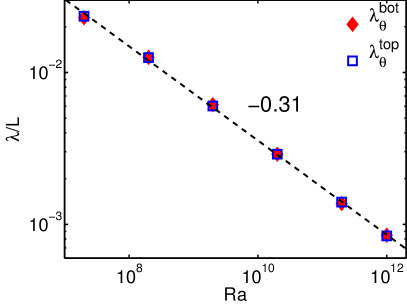
We determined the thermal and kinetic BL thickness for the simulations in the $\Gamma=0.23$ sample. The horizontally averaged thermal BL thickness ($\lambda_{\theta}$) is determined from $\lambda_{\theta}^{sl}(r)$, where $\lambda_{\theta}^{sl}(r)$ is the intersection point between the linear extrapolation of the temperature gradient at the plate with the behavior found in the bulk (Stevens et al. (2010a)). In figure 5a it is shown that the scaling of the thermal BL thickness is consistent with the $Nu$ number measurements when the horizontal average is taken over the entire plate.

Figure 5: BL thicknesses for $Pr=0.7$ in the $\Gamma=0.23$ sample. a) The thermal BL thickness close to the bottom and top plate averaged over the entire horizontal area scales with $Ra^{-0.31}$ (black dashed line) b) The kinetic (dark green line) and thermal (black line) BL thicknesses averaged between $0.25D/2<r<0.50D/2$ scale with $Ra^{-0.26}$. Note that this is slightly less than in figure 5, when we average $\lambda_{\theta}$ over the full area.

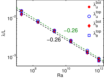
The horizontally averaged kinetic BL thickness ($\lambda_{u}$) is determined from $\lambda_{u}^{"}(r)$, where $\lambda_{u}^{"}(r)$ is based on the position where the quantity $\epsilon_{u}^{"}:=\bf{u}\cdot\nabla^{2}\bf{u}$ reaches its maximum. We use this quantity as Stevens et al. (2010b) and Shishkina et al. (2010) showed that it represents the kinetic BL thickness better than other available methods. Stevens et al. (2010a, b) also explained that this quantity cannot be used close to the sidewall as here it misrepresents the kinetic BL thickness. For numerical reasons, it can neither be calculated accurately in the center region. To be on the safe side we horizontally average the kinetic BL between $0.25D/2<r<0.75D/2$, where $D$ indicates the diameter of the cell and all given values refer to that used.

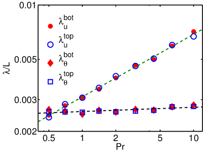
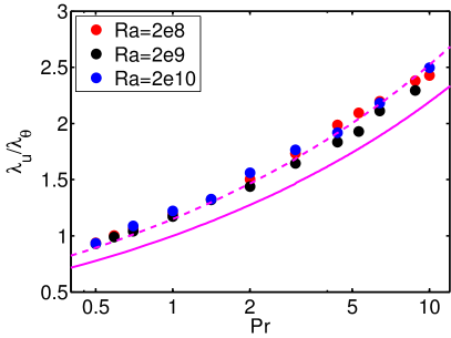
Figure 5b reveals that for $Pr=0.7$ the kinetic and thermal BL thickness have the same scaling and thickness over a wide range of $Ra$. In figure 6 the ratio $\lambda_{u}/\lambda_{\theta}$ is compared with results of the Prandtl-Blasius BL theory. We find a constant difference of about $15\%$ between the numerical results and the theoretical PB type prediction, see e.g. Shishkina et al. (2010). We emphasize that the deviation of the prefactor of only 15% is remarkably small, given that the PB boundary layer theory has been developed for parallel flow over an infinite flat plate, whereas here in the aspect ratio $\Gamma=0.23$ cell one can hardly find such regions of parallel flows at the top and bottom plates. Nonetheless, the scaling and even the ratio of the kinetic and thermal boundary layer thicknesses for these large $Ra$ numbers is well described by Prandtl-Blasius BL theory. This result agrees with the experimental results of Qiu & Xia (1998) and Sun et al. (2008). Indeed, Qiu & Xia (1998) showed that the kinetic BL near the sidewall obeys the scaling law of the Prandtl-Blasius laminar BL and Sun et al. (2008) showed the same for the boundary layers near the bottom plate. Recently, Zhou & Xia (2010); Zhou et al. (2010) have developed a method of expressing velocity profiles in the time-dependent BL frame and found that not only the scaling obeys the PB expectation, but even the rescaled velocity and temperature profiles From all this we can exclude that at $Ra\lesssim 10^{12}$ the BL is turbulent.

Figure 6: a) Kinetic and thermal BL thicknesses close to the bottom and top plate for $Ra=2\times 10^{10}$. b) The ratio between the kinetic and thermal BL thickness as function of $Pr$ for different $Ra$. The green solid line indicates the prediction from the Prandtl-Blasius theory (Shishkina et al. (2010)). The green dashed line, which lies $15\%$ above the theoretical prediction, is a guide to the eye. All numerical data are horizontally averaged for $0.25D/2<r<0.50D/2$.

5 Constant temperature versus constant heat flux condition at the bottom plate

It has also been argued that the different boundary conditions at the bottom plate, i.e. that some experiments are closer to a constant temperature boundary condition, and some are closer to a constant heat flux boundary condition, might explain the differences in the heat transport that are observed in the high $Ra$ number regime. Figure 7a compares the $Nu$ number in the simulations with constant temperature and constant heat flux at the bottom plate. The figure shows that the difference between these both cases is small and even decreases with increasing $Ra$. For large $Ra$ no difference at all is seen within the (statistical) error bars, which however increase due to the shorter averaging time (in terms of large eddy turnovers) at the very large $Ra\geq 2\times 10^{11}$.

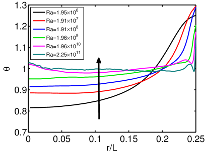
Figure 7b shows the time-averaged temperature of the bottom plate in the simulations with constant heat flux at the bottom plate for different $Ra$. The radial dependence at the lower $Ra$ numbers can be understood from the flow structure in the sample: Due to the large scale circulation the fluid velocities are largest in the middle of the sample. Thus in the middle more heat can be extracted from the plate than close to the sidewall where the fluid velocities are smaller. It is the lack of any wind in the corners of the sample that causes the relative high time-averaged plate temperature there. The figure also shows that this effect decreases with increasing $Ra$. The reason for this is that the turbulence becomes stronger at higher $Ra$ and this leads to smaller flow structures. Therefore the region close to the sidewall with relative small fluid velocities decreases with increasing $Ra$ and this leads to a more uniform plate temperature at higher $Ra$. This effect explains that the simulations with constant temperature and constant heat flux condition at the bottom plate become more similar with increasing $Ra$.

The small differences between the simulations with constant temperature and constant heat flux at the bottom plate shows that the differences between the experiments in the high $Ra$ number regime can not be explained by different plate conductivity properties. This finding is in agreement with the results of Johnston & Doering (2009). In their periodic two-dimensional RB simulations the heat transfer for simulations with constant temperature and constant heat flux (both at the bottom and the top plate) becomes equal at $Ra\approx 5\times 10^{6}$. For the three-dimensional simulations the heat transfer for both cases also becomes equal, but at higher $Ra$. This is due to the geometrical effect discussed before, see figure 7b, that cannot occur in periodic two-dimensional simulations (Johnston & Doering (2009)).

Figure 7: a) $Nu$ vs $Ra$ for $\Gamma=0.5$. Data as in figure 2a. The numerical data for $Pr=0.7$ with constant heat flux at the bottom and constant temperature at the top plate are indicted in blue and the numerical data with constant temperature condition at both plates in black. b) Time-averaged temperature at the bottom plate for simulations with constant heat flux at the bottom plate and constant temperature at the top plate. The arrow indicates the direction of increasing $Ra$.

6 Conclusions

In summary, we presented results from three-dimensional DNS simulations for RB convection in cylindrical samples of aspect ratios $\Gamma=0.23$ and $\Gamma=0.5$ up to $Ra=2\times 10^{12}$ and a broad range of $Pr$ numbers. The simulation at $Ra=2\times 10^{12}$ with $Pr=0.7$ in an aspect ratio $\Gamma=0.5$ sample is in good agreement with the experimental results of Niemela et al. (2000, 2001), Niemela & Sreenivasan (2006), Funfschilling et al. (2009), and Ahlers et al. (2009a, b), while there is a visible difference with the results of Chavanne et al. (2001). In addition, we showed that the differences in the heat transfer observed between experiments for $Ra\gtrsim 2\times 10^{11}$ can neither be explained by $Pr$ number effects, nor by the assumption of constant heat flux conditions at the bottom plate instead of constant temperature conditions. Furthermore, we demonstrated that the scaling of the kinetic and thermal BL thicknesses in this high $Ra$ number regime is well described by the Prandtl-Blasius theory.

Several questions remain: Which effect is responsible for the observed difference in $Nu$ vs $Ra$ scaling in the various experiments? Are there perhaps different turbulent states in the highly turbulent regime as has been suggested for RB flow by Grossmann & Lohse (2011), but also for other turbulent flows in closed systems by Cortet et al. (2010)? At what $Ra$ number do the BLs become turbulent? As in DNSs both the velocity and temperature fields are known in the whole domain (including in the boundary layers where the transition between the states is suggested to take place), they will play a leading role in answering these questions.