Abstract

Scalar cosmological perturbations with nearly flat power spectrum may originate from perturbations of the phase of a scalar field conformally coupled to gravity and rolling down negative quartic potential. We consider a version of this scenario whose specific property is a long intermediate stage between the end of conformal rolling and horizon exit of the phase perturbations. Such a stage is natural, e.g., in cosmologies with ekpyrosis or genesis. Its existence results in small negative scalar tilt, statistical anisotropy of all even multipoles starting from quardupole of general structure (in contrast to the usually discussed single quadrupole of special type) and non-Gaussianity of a peculiar form.

1 Introduction and summary

By far the most developed hypothesis on the origin of the cosmological perturbations is the slow roll inflation [1]. The inflationary mechanism [2] generates almost Gaussian scalar perturbations whose power spectrum is almost flat due to the slow evolution of relevant parameters (the Hubble parameter and time derivative of the inflaton field). Similar situation occurs in the inflationary scenario with the curvaton mechanism [3]; in either case, the approximate flatness of the spectrum is a direct consequence of the approximate de Sitter symmetry of the inflating background.

In quest for an alternative symmetry behind the flat scalar spectrum one naturally turns to conformal invariance [4, 5]. Conformal symmetry implies scale invariance, which in the end may be responsible for the scale-invariant scalar spectrum. An assumption of conformal invariance at the time the primordial perturbations are generated is in line with the viewpoint that the underlying theory of Nature may have conformal phase, and that the Universe may have started off from, or passed through that phase.

At the present, exploratory stage it makes sense to consider this possibility in the context of toy models. One such model is proposed in Ref. [4]. Besides conventional Einstein gravity and some matter that dominates the cosmological evolution, its main ingredient is a complex scalar field $\phi$ conformally coupled to gravity. Conformal invariance implies that the scalar potential is quartic, while the dynamics is non-trivial if its sign is negative,

$$V(\phi)=-h^{2}|\phi|^{4}\;,$$ (1)

where $h$ is a small parameter. One assumes that the background space-time is homogeneous, isotropic and spatially flat,

$$ds^{2}=a^{2}(\eta)(d\eta^{2}-d{\bf x}^{2})\;.$$ (2)

Then in terms of the field

$$\chi(\eta,{\bf x})=a(\eta)\phi(\eta,{\bf x})$$

the dynamics is the same as in flat space-time. One further assumes that the classical background field $\chi_{c}$ is homogeneous. As it rolls down its potential $V(\chi)=-h^{2}|\chi|^{4}$, it approaches the late time attractor

$$\chi_{c}(\eta)=\frac{1}{h(\eta_{*}^{(0)}-\eta)}\;,$$ (3)

where $\eta_{*}^{(0)}$ is an arbitrary real parameter (“end of roll”; the reason for the superscript $(0)$ in notation will become clear later), and we take $\chi_{c}$ real without loss of generality.

The point of Ref. [4] is that the behavior of the phase $\theta=\sqrt{2}\;\mbox{Arg}\;\phi$ in the background (3) is very similar to what happens at inflation to the fluctuations of a massless scalar field minimally coupled to gravity (e.g., inflaton itself). The phase perturbations $\delta\theta$ start off as vacuum fluctuations and eventually freeze out. To the leading order in $h$, the resulting phase perturbations are Gaussian and have flat power spectrum

$${\cal P}_{\delta\theta}=\frac{h^{2}}{(2\pi)^{2}}\;.$$ (4)

The latter property is a consequence of conformal invariance and $U(1)$-symmetry $\phi\to\mbox{e}^{i\alpha}\phi$ inherent in the model. The phase perturbations are the source of the adiabatic perturbations in this scenario, which proceeds as follows. At large field values, the potential $V(|\phi|)$ is assumed to be different from (1) and to have a minimum at $|\phi|=f_{0}$; we assume that $f_{0}\ll M_{\mathrm{PL}}$ (see also the discussion in Section 2.1), so that the contribution of the field $\phi$ to the effective Planck mass is always negligible. At $|\phi|\sim f_{0}$, conformal symmetry is broken, the radial field $|\phi|$ interacts with other fields, and its oscillations about the minimum get damped quickly enough. To be on the safe side, we assume that the field $\phi$ is a spectator at this and earlier stages, i.e., its energy density $\rho_{\phi}$ is small compared to the energy density $\rho_{\mathrm{tot}}$ of matter that dominates the cosmological evolution. This is the case provided that

$$|\rho_{\phi}|\sim h^{2}f_{0}^{4}\ll\rho_{\mathrm{tot}}=\frac{3}{8\pi}M_{\mathrm{PL}}^{2}H^{2}\;.$$ (5)

Then the decay products of the field $|\phi|$ do not affect the evolution of the Universe and, furthermore, the perturbations of $|\phi|$, that exist before the end of rolling and disappear after $|\phi|$ gets relaxed to the minimum of $V(|\phi|)$, do not produce substantial density perturbations in the Universe.

Once the radial field $|\phi|$ settles down to $f_{0}$, what remains are the perturbations of the phase, which at this point are isocurvature perturbations. They get reprocessed into adiabatic perturbations at much later epoch by one or another mechanism. As an example, the phase $\theta$ may be pseudo-Nambu–Goldstone field, and may serve as curvation [3, 6]. Alternatively, perturbations $\delta\theta$ may be converted into adiabatic perturbations by the modulated decay mechanism [7, 8]. In either case, the adiabatic perturbations inherit the correlation properties from the phase perturbations (with possible additional non-Gaussianity generated at the conversion epoch), while the amplitude of the adiabatic perturbations is, generally speaking, smaller than that of the phase perturbations. In view of the latter property, we treat our only parameter, the coupling constant $h$, as free (but small).

The scenario cannot work at the conventional hot cosmological epoch, for the following reason. The vacuum state of the phase perturbations $\delta\theta$ is well defined at early times provided that these perturbations evolve in the WKB regime, which implies

$$k(\eta_{*}^{(0)}-\eta)\gg 1\;,\;\;\;\;\;\mbox{early~{}times}\;,$$ (6)

where $k$ is conformal momentum. On the other hand, the property that these perturbations are frozen out at late times holds if

$$k(\eta_{*}^{(0)}-\eta)\ll 1\;,\;\;\;\;\;\mbox{late~{}times}\;.$$ (7)

So, the scenario requires that both of these inequalities are satisfied at conformal rolling stage. This can only happen if the duration of that stage in conformal time is greater than $k^{-1}$. For conformal momenta of cosmological significance this means that conformal rolling lasts longer (in conformal time) than the entire hot stage until the present epoch. Thus, the mechanism can only work at some pre-hot epoch at which the horizon problem is solved, at least formally. This is similar to most other mechanisms of the generation of cosmological perturbations (see, however, Ref. [9]).

At the conformal rolling stage, the dynamics of the phase perturbations $\delta\theta$ is governed solely by their interaction with the background field (3) (as well as with the radial perturbations $\delta|\chi|$, see below); the evolution of the scale factor $a(\eta)$ is irrelevant. After the end of conformal rolling, the situation is reversed. Once the radial field $|\phi|$ has relaxed to the minimum of the scalar potential, the phase $\theta$ is a massless scalar field minimally coupled to gravity (this is true for any Nambu–Goldstone field [10]). Since we are talking about a yet unknown pre-hot epoch, it is legitimate to ask what happens to the perturbations of the phase right after the end of conformal rolling. Barring fine tuning, there are two possibilities for the perturbations $\delta\theta$:

(i) they are already superhorizon in the conventional sense at that time, or

(ii) they are still subhorizon.

The version (i) of the scenario has been considered in Refs. [11, 12]; in that case, the phase perturbations do not evolve after the end of the conformal rolling stage, and the properties of the adiabatic perturbations are determined entirely by the dynamics at conformal rolling (modulo possible non-Gaussianity generated at the conversion epoch; the latter is not specific to the conformal rolling scenario). To subleading orders in $h$, this dynamics is fairly non-trivial, and the resulting effects include certain types of statistical anisotropy [11] and non-Gaussianity [12].

In this paper we consider the second possibility, i.e., assume that there is a long enough period of time after the end of conformal rolling, at which the phase perturbations remain subhorizon in the conventional sense. Their behavior between the end of conformal rolling and horizon exit depends strongly on the evolution of the scale factor at this intermediate stage. In order that the flat power spectrum (4) be not grossly modified at this epoch, the scale factor should evolve in such a way that the dynamics of $\delta\theta$ is effectively nearly Minkowskian. Although this requirement sounds prohibitively restrictive, there are at least two cosmological scenarios in which it is obeyed. One is the bouncing Universe, with matter at the contracting stage having super-stiff equation of state, $p\gg\rho$. It is worth noting in this regard that stiff equation of state is preferred at the contracting stage for other reasons [13, 14] and is inherent, e.g., in a scalar field theory with negative exponential potential, like in the ekpyrotic model [15]. It is known [16] that in models with super-stiff matter at contracting stage, the resulting power spectrum of scalar perturbations is almost the same as that of massless scalar field in Minkowski space, ${\cal P}(k)\propto k^{2}$. This implies that the dynamics of the scalar field perturbations is almost Minkowskian in these models. We discuss this point further in Appendix A. In tractable bouncing models like those of Refs. [17, 18, 19], our phase perturbations exit the horizon at the contracting stage, pass through the bounce unaffected (cf. Ref. [20]), remain superhorizon early at the hot expansion epoch and get reprocessed into adiabatic perturbations, as discussed above.

Similar situation occurs in another scenario suitable for our purposes, namely, “genesis” of Ref. [5] (see also Ref. [17]). According to this scenario, the Universe is initially spatially flat and nearly static, stays in this nearly Minkowskian state for long time, then its expansion quickly speeds up and eventually the conventional hot epoch begins. If our conformal rolling stage ends up well before the start of rapid expansion, the evolution of the phase perturbations is again nearly Minkowskian up until the horizon exit.

In both scenarios the relevant range of momenta is wide, provided that $f_{0}$ is small enough (but not unrealistically small). We discuss this point in Section 2.1. So, it is legitimate to approximate the evolution of the phase perturbations as Minkowskian in the time interval $\eta_{*}-\epsilon<\eta<\eta_{1}$, where $\eta_{1}$ is some time after the horizon exit, and $(\eta_{*}-\epsilon)$ is the time when the radial field relaxes to the minimum of $V(|\phi|)$ and the conformal rolling stage ends. We set $\epsilon=0$ in what follows to simplify notations; keeping $\epsilon\neq 0$ would not change our results (recall that the phase perturbations are frozen out well before $\eta=\eta_{*}$). The field $\delta\theta({\bf x},\eta_{*})$, determined by the dynamics at the conformal rolling stage, serves as the initial condition for further Minkowskian evolution from $\eta_{*}$ to $\eta_{1}$. Barring fine tuning, the case of interest for us is

$$k(\eta_{1}-\eta_{*})\gg 1\;.$$

Our purpose is to study the properties of the phase perturbations at $\eta=\eta_{1}$, as these properties are inherited by the adiabatic perturbations.

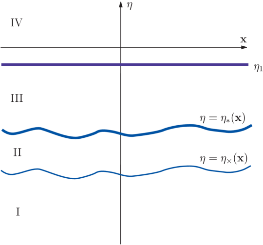
To the leading order in $h$, we find nothing new: the phase perturbations at $\eta=\eta_{1}$ are Gaussian and have flat power spectrum. Subleading orders in $h$ are more interesting. A simple way to understand what is going on is to notice that the end-of-roll time $\eta_{*}$, instead of being a constant parameter, is actually a Gaussian random field [4], $\eta_{*}({\bf x})=\eta_{*}^{(0)}+\delta\eta_{*}({\bf x})$ with $\delta\eta_{*}\propto h$. This is due to the fact that not only the phase $\theta$ but also the radial field $|\chi|$ acquire perturbations at the conformal rolling stage; after freeze out, perturbations $\delta|\chi|$ can be interpreted as perturbations $\delta\eta_{*}({\bf x})$. The effect of the perturbations $\delta\eta_{*}$ on the phase perturbations $\delta\theta$ is twofold. First, the perturbations $\delta\eta_{*}$ modify the dynamics of $\delta\theta$ at the conformal rolling stage. This property is common to both cases (i) and (ii), and we make use of the results of Ref. [11]. The new point is that the resulting field $\delta\theta({\bf x},\eta_{*}({\bf x}))$ serves as the initial condition for the Minkowskian evolution. Second, this initial condition is now imposed at the non-trivial hypersurface $\eta=\eta_{*}({\bf x})$. This is illustrated in Fig. 1.

Figure 1: Due to the perturbations of the radial field, the evolution of phase perturbations proceeds in inhomogeneous background. Perturbations $\delta\theta$ oscillate in time at early stage (region I), freeze out at time $\eta=\eta_{\times}({\bf x})$ and temporarily stay constant (region II) until the end of conformal rolling that occurs at $\eta=\eta_{*}({\bf x})$. Then they evolve again, now in nearly Minkowskian regime (region III), until the horizon exit time $\eta_{1}$. Later on (region IV), perturbations $\delta\theta$ are superhorizon and stay constant.

The net result is that the perturbation $\delta\theta({\bf x})$ at the time $\eta_{1}$ is a combination of two Gaussian random fields originating from vacuum fluctuations of the phase $\theta$ and radial field $|\chi|$, respectively (better to say, from vacuum fluctuations of imaginary and real parts of $\chi$, with our convention of real background $\chi_{c}$). This leads to several potentially observable effects.

At the level of the two-point correlation function of the phase perturbation $\delta\theta({\bf x},\eta_{1})$, and hence of the adiabatic perturbation $\zeta$, we have found two effects. The first one is negative scalar tilt

$$n_{s}-1=-\frac{3h^{2}}{4\pi^{2}}\;.$$ (8)

We note in passing that this is not a particularly strong result, as small scalar tilt in our scenario may also originate from weak violation of conformal invariance at the conformal rolling stage [21] and/or not exactly Minkowskian evolution of $\delta\theta$ at the intermediate stage, cf. Appendix A. The second effect is the statistical anisotropy: the power spectrum has the form

$${\cal P}_{\zeta}({\bf k})={\cal P}_{\zeta}^{(0)}(k)\left[1+Q(\hat{\bf k})\right]\;,$$ (9)

where ${\cal P}_{\zeta}^{(0)}$ is independent of the direction of momentum (nearly flat spectrum with small tilt), $\hat{\bf k}={\bf k}/k$ is the unit vector along the momentum and $Q(\hat{\bf k})$ is itself a random field, which depends on the direction of ${\bf k}$ only. Unlike the statistical anisotropy discussed in the inflationary context [22, 23, 24, 25], and also in the version (i) of the conformal rolling scenario [11], the function $Q(\hat{\bf k})$ contains all even angular harmonics, starting from quadrupole. We give here the expression for $Q(\hat{\bf k})$ which accounts for the quadrupole component only (see Section 4 for the results valid for all multipoles)

$$Q(\hat{k})={\cal Q}\cdot w_{ij}\left(\hat{k}_{i}\hat{k}_{j}-\frac{1}{3}\delta_{ij}\right)\;,$$ (10)

where $w_{ij}$ is a general symmetric traceless tensor normalized to unity, $w_{ij}w_{ij}=1$, and the variance of the quadrupole component (in the sense of an ensemble of universes) is

$$\langle{\cal Q}^{2}\rangle=\frac{225h^{2}}{32\pi^{2}}$$ (11)

Of course, the precise values of the multipoles of $Q(\hat{\bf k})$ in our patch of the Universe are undetermined because of the cosmic variance.

Due to the interaction with the perturbations $\delta\eta_{*}$, the resulting phase perturbations $\delta\theta({\bf x},\eta_{1})$ and their descendant perturbations $\zeta$ are non-Gaussian (we leave aside here the non-Gaussianity that may be generated at the epoch of conversion of the phase perturbations into adiabatic ones; our scenario is not special in this respect). Their three-point correlation function vanishes identically due to the discrete symmetry $\theta\to-\theta$ (cf. Ref. [11]), while the four-point correlation function has a peculiar form

$$\langle\zeta({\bf k}) \zeta(\tilde{\bf k})\zeta({\bf k}^{\prime})\zeta(\tilde{\bf k}^{\prime})\rangle=\frac{{\cal P}_{\zeta}^{(0)}(k)}{4\pi k^{3}}\frac{{\cal P}_{\zeta}^{(0)}(k^{\prime})}{4\pi k^{\prime\,3}}\delta({\bf k}+\tilde{\bf k})\delta({\bf k}^{\prime}+\tilde{\bf k}^{\prime})\cdot\left[1+F_{NG}(\hat{\bf k},\hat{\bf k}^{\prime})\right]$$

$$~{}~{}~{}~{}~{}~{}~{}~{}~{}~{}~{}~{}~{}~{}~{}~{}~{}~{}~{}~{}~{}~{}~{}~{}~{}~{}~{}~{}~{}~{}~{}~{}~{}~{}~{}~{}~{}~{}~{}~{}~{}~{}~{}~{}~{}~{}~{}~{}~{}~{}~{}~{}~{}~{}~{}+({\bf k}\leftrightarrow{\bf k}^{\prime})+(\tilde{\bf k}\leftrightarrow{\bf k}^{\prime})\;.$$ (12)

The leading term in (12) (unity in square brackets) is the Gaussian part, while the non-Gaussianity is encoded in $F_{NG}=O(h^{2})$. Note that the structure of the non-Gaussian part is fairly similar to that of the disconnected four-point function. Note also that $F_{NG}$ depends on the angle between ${\bf k}$ and ${\bf k}^{\prime}$ only. For reasons we discuss in Section 5, the notion of non-Gaussianity is appropriate if the angle between ${\bf k}^{\prime}$ and ${\bf k}$ is small, i.e., $|\hat{\bf k}-\hat{\bf k}^{\prime}|\ll 1$. In this regime, the leading behaviour of $F_{NG}$ is

$$F_{NG}=\frac{3h^{2}}{\pi^{2}}\log\frac{\mbox{const}}{|\hat{\bf k}-\hat{\bf k}^{\prime}|}\;,$$

where constant in the argument of logarithm cannot be reliably calculated because of the cosmic variance. The logarithmic behavior does not hold for arbitrarily small $|\hat{\bf k}-\hat{\bf k}^{\prime}|$: the function $F_{NG}(\hat{\bf k}-\hat{\bf k}^{\prime})$ flattens out most likely at $|\hat{\bf k}-\hat{\bf k}^{\prime}|\sim[k(\eta_{1}-\eta_{*})]^{-1/2}$, and certainly at $|\hat{\bf k}-\hat{\bf k}^{\prime}|\sim[k(\eta_{1}-\eta_{*})]^{-1}$. So, the parameter $(\eta_{1}-\eta_{*})$ is detectable in principle (but, probably, not in practice).

It is tempting to speculate that the negative scalar tilt $n_{s}-1\simeq-0.04$, favoured by the data [26], has its origin in the dynamics we discuss in this paper. If so, our only free parameter $h$ is determined from (8), $h^{2}\simeq 0.5$, while the small amplitude of the adiabatic perturbations is to be attributed to the mechanism that reprocesses the phase perturbations into adiabatic ones. In that case the statistical anisotropy is roughly of order 1, which is probably inconsistent with the data. On the other hand, if one attributes the small observed amplitude of primordial scalar perturbations, $\sqrt{{\cal P}_{\zeta}}\simeq 5\cdot 10^{-5}$ [27], entirely to the smallness of $h$, i.e., identifies ${\cal P}_{\delta\theta}$ with ${\cal P}_{\zeta}$, then $h^{2}\sim 10^{-7}$, and the statistical anisotropy is at the level $Q\sim 10^{-3}$, while the non-Gaussianity is probably unobservable. This gives an idea of the range of predictions of our model.

This paper is organized as follows. We begin in Section 2.1 with discussing the range of momenta of modes under study. To make the presentation self-contained, we review in Sections 2.2 – 2.4 the properties of the radial and phase perturbations at the conformal rolling stage [11]. Phase perturbations at the end of intermediate, (almost) Minkowskian stage are studied in Section 3 to the first non-trivial order in $h$. This is sufficient for evaluating the statistical anisotropy and non-Gaussianity in Sections 4 and 5, respectively. The calculation of the tilt (8) requires the analysis of order-$h^{2}$ corrections, so we postpone it to Section 6. We discuss in Appendix A the properties of a massless scalar field in the contracting Universe filled with super-stiff matter. We present in Appendices B – D technical details of the calculations performed in Sections 3 and 4.

2 Conformal rolling

Let us review the main properties of our scalar field at the stage when it rolls down its potential. At this stage, the theory is described by the action

$$S=S_{G+M}+S_{\phi}\;,$$

where $S_{G+M}$ is the action for gravity and some matter that dominates the evolution of the Universe, and

$$S_{\phi}=\int d^{4}x\sqrt{-g}\left[g^{\mu\nu}\partial_{\mu}\phi^{*}\partial_{\nu}\phi+\frac{R}{6}\phi^{*}\phi-V(\phi)\right]\;$$

is the action for the scalar field we are going to discuss. Here the scalar potential is given by (1). We assume that the field $\phi$ is a spectator which does not affect the cosmological evolution; for this reason, mixing between this field and gravitational degrees of freedom is negligible. The background metric is assumed to be given by (2). One introduces the field $\chi=a\phi$, and obtains its action in conformal coordinates in the Minkowskian form,

$$S[\chi]=\int~{}d^{3}x~{}d\eta~{}\left[\eta^{\mu\nu}\partial_{\mu}\chi^{*}\partial_{\nu}\chi+h^{2}|\chi|^{4}\right]\;.$$

The homogeneous background solution $\chi_{c}(\eta)$ to the field equation is given by (3). Recall that we have chosen $\chi_{c}$ real without loss of generality.

2.1 Momentum scales

Before discussing field perturbations in detail, let us consider momentum scales for which our scenario, outlined in Section 1, is valid. According to this scenario, conformal rolling stage ends up when the radial field $|\phi|$ becomes of order $f_{0}$. This occurs at time $\eta_{f}$ such that

$$\frac{1}{a(\eta_{f})h(\eta_{f}-\eta_{*}^{(0)})}\sim f_{0}\;.$$

Hence, the shortest waves obeying (7) have present momenta

$$\frac{k_{\mathrm{max}}}{a_{0}}\sim hf_{0}\cdot\frac{a(\eta_{f})}{a_{h}}\cdot\frac{a_{h}}{a_{0}}\;,$$

where $a_{0}$ and $a_{h}$ are the present value of the scale factor and its value at the beginning of the hot stage, respectively. On the other hand, we assume that the relevant modes are subhorizon right after $\eta_{f}$,

$$\frac{k}{a(\eta_{f})}>H(\eta_{f})\;.$$ (13)

We recall our requirement (5) and find that the longest waves obeying (13) satisfy

$$\frac{k}{a_{0}}>\frac{k_{\mathrm{min}}}{a_{0}}\sim\frac{hf_{0}^{2}}{M_{\mathrm{PL}}}\cdot\frac{a(\eta_{f})}{a_{h}}\cdot\frac{a_{h}}{a_{0}}\;.$$ (14)

We see that the relevant range of momenta is

$$\frac{f_{0}}{M_{\mathrm{PL}}}\cdot k_{\mathrm{max}}<k<k_{\mathrm{max}}\;.$$

It is wide enough, provided that the energy scale $f_{0}$ is sufficiently low. As an example, for $k_{\mathrm{max}}/k_{\mathrm{min}}\sim(10\mathrm{kpc})^{-1}/(10\mathrm{Gpc})^{-1}$ we need $f_{0}<10^{-6}M_{\mathrm{PL}}$.

If our mechanism is supposed to work at contracting stage in the bouncing Universe scanario with the hot epoch starting immediately after bounce, the inequality (14) implies much stronger bound on $f_{0}$. Indeed, $a(\eta_{f})/a_{h}>1$ in this scenario, while $a_{h}/a_{0}\gtrsim T_{0}/T_{h}>T_{0}/M_{\mathrm{PL}}$. We require that $k_{\mathrm{min}}/a_{0}$ is lower than the present Hubble scale $H_{0}$ and obtain

$$\sqrt{h}\cdot f_{0}<M_{\mathrm{PL}}\left(\frac{H_{0}}{T_{0}}\right)^{1/2}\sim 10^{-15}M_{\mathrm{PL}}\;.$$ (15)

Even for $h\sim 10^{-4}$ this implies $f_{0}<10^{6}\mathrm{GeV}$. Interestingly, fully consistent with this scenario is the scale $f_{0}\sim\mathrm{TeV}$.

On the contrary, $a(\eta_{f})/a_{h}$ can be large in the “genesis” scenario [5]. Therefore, no bound similar to (15) can be established in that case.

2.2 Radial perturbations

Let us consider perturbations about this background. To the leading order in $h$, perturbations $\delta\chi_{1}=\sqrt{2}\delta(\mbox{Re}\,\chi)$ and $\delta\chi_{2}=\sqrt{2}\mbox{Im}\,\chi$ decouple from each other. At early times, when the relation (6) is satisfied, the fields $\delta\chi_{1}$ and $\delta\chi_{2}$ are free and Minkowskian. The vacuum is well defined and we assume, as usual, that this vacuum is the initial state. The normalization factor $\sqrt{2}$ is chosen in such a way that the real fields $\delta\chi_{1}$ and $\delta\chi_{2}$ are canonically normalized at early times. At late times, when the opposite inequality (7) holds, the perturbations no longer oscillate.

We begin with the radial perturbations $\delta\chi_{1}$. They obey the linearized field equation, in momentum representation,

$$(\delta\chi_{1})^{\prime\prime}+p^{2}~{}\delta\chi_{1}-6h^{2}\chi_{c}^{2}\delta\chi_{1}\equiv(\delta\chi_{1})^{\prime\prime}+p^{2}~{}\delta\chi_{1}-\frac{6}{(\eta_{*}^{(0)}-\eta)^{2}}\delta\chi_{1}=0\;,$$ (16)

where prime denotes the derivative with respect to conformal time. We denote the conformal momentum of the radial perturbation by ${\bf p}$ and reserve the notation ${\bf k}$ for the conformal momentum of the phase perturbation. The properly normalized solution to Eq. (16) is

$$\delta\chi_{1}=\frac{1}{4\pi}\sqrt{\frac{\eta_{*}^{(0)}-\eta}{2}}H_{5/2}^{(1)}\left[p(\eta_{*}^{(0)}-\eta)\right]\cdot\hat{B}_{\bf p}+h.c.\;,$$

where $\hat{B}_{\bf p}$, $\hat{B}_{\bf p}^{\dagger}$ are annihilation and creation operators obeying the standard commutational relation $[\hat{B}_{\bf p},\hat{B}_{{\bf p}^{\prime}}^{\dagger}]=\delta({\bf p}-{\bf p}^{\prime})$, $H_{5/2}^{(1)}$ is the Hankel function, and here and in what follows in this Section we omit irrelevant phase factors. At late times the solution approaches the asymptotics

$$\delta\chi_{1}=\frac{3}{4\pi^{3/2}}\frac{1}{p^{5/2}(\eta_{*}^{(0)}-\eta)^{2}}\cdot\hat{B}_{\bf p}+h.c.\;.$$

The interpretation of the behaviour $\delta\chi_{1}\propto(\eta_{*}^{(0)}-\eta)^{-2}$ is that the end-of-roll parameter $\eta_{*}$ becomes a random field. Indeed, with perturbations included, the radial field $\mbox{Re}\,\chi=\chi_{c}+\delta\chi_{1}/\sqrt{2}$ can be written at late times as follows,

$$\mbox{Re}\,\chi=\frac{1}{h[\eta_{*}({\bf x})-\eta]}\;,$$ (17)

where

$$\eta_{*}({\bf x})=\eta_{*}^{(0)}+\delta\eta_{*}({\bf x})$$

and the linearization in $\delta\eta_{*}$ is understood. The field $\delta\eta_{*}$ is constant in time and is given by

$$\delta\eta_{*}({\bf x})=\frac{3h}{4\sqrt{2}\pi^{3/2}}\int~{}\frac{d^{3}p}{p^{5/2}}\left(\mbox{e}^{i{\bf px}}\cdot\hat{B}_{\bf p}+h.c.\right)\;.$$

Note that this field has red power spectrum,

$${\cal P}_{\delta\eta_{*}}=\frac{9h^{2}}{8\pi^{2}}\frac{1}{p^{2}}\;.$$ (18)

Clearly, the overall spatially homogeneous shift of the end-of-roll time is irrelevant, as it can be absorbed into redefinition of the bare parameter $\eta_{*}^{(0)}$. What is important is the gradient of $\eta_{*}({\bf x})$, as well as higher derivatives. It is convenient to introduce the notation

$$v_{i}=-\partial_{i}\eta_{*}({\bf x})\;.$$

It reflects the fact that to the first order in the gradient expansion of $\eta_{*}({\bf x})$ (i.e., neglecting the second derivatives of $\eta_{*}({\bf x})$) and to the linear order in ${\bf v}$, the hypersurfaces of constant $\mbox{Re}\,\chi$, i.e., hypersurfaces $\eta_{*}({\bf x})-\eta=\mbox{const}$, are boosted with the velocity ${\bf v}$ with respect to the cosmic frame: these are hypersurfaces $\eta+{\bf vx}=\mbox{const}$. The random field ${\bf v}({\bf x})$ has flat power spectrum, while higher derivatives of $\eta_{*}({\bf x})$ have blue spectra.

2.3 Phase perturbations: order $v$

Let us now turn to the perturbations $\delta\chi_{2}$ of the imaginary part, and account for their interaction with radial perturbations. As we will see in what follows, relevant perturbations $\delta\eta_{*}$ have wavelengths much longer than the wavelengths of the phase perturbations,

$$p\ll k\;,$$

where, as before, ${\bf p}$ and ${\bf k}$ are conformal momenta of radial and phase perturbations, respectively. Because of this separation of scales, it is legitimate to use the expression (17), valid in the late-time regime $p(\eta_{*}-\eta)\ll 1$, when considering the dynamics of $\delta\chi_{2}$, and treat the field (17) as the background. It is worth noting, however, that the expression (17) is valid to the linear order in $\delta\eta_{*}$ only; furthermore, there are corrections to (17) of order $\partial_{i}\partial_{j}\eta_{*}({\bf x})/(\eta_{*}-\eta)$. Therefore, the results of this Section are valid to order $v$ (or, equivalently, to the subleading order in $h$). We present the expressions valid to order $v^{2}$ in Section 2.4.

With this qualification, the linearized field equation for $\delta\chi_{2}$ reads

$$(\delta\chi_{2})^{\prime\prime}-\partial_{i}\partial_{i}\;\delta\chi_{2}-2h^{2}(\mbox{Re}\,\chi)^{2}\cdot\delta\chi_{2}\equiv(\delta\chi_{2})^{\prime\prime}-\partial_{i}\partial_{i}\;\delta\chi_{2}-\frac{2}{[\eta_{*}({\bf x})-\eta]^{2}}\delta\chi_{2}=0\;.$$ (19)

At early times, when $k(\eta_{*}-\eta)\gg 1$, we get back to the Minkowskian massless equation, and the solutions are spatial Fourier modes that oscillate in time. Hence, the solution to Eq. (19) has the following form,

$$\delta\chi_{2}({\bf x},\eta)=\int~{}\frac{d^{3}k}{(2\pi)^{3/2}\sqrt{2k}}~{}\left(\delta\chi_{2}^{(-)}({\bf k},{\bf x},\eta)\hat{A}_{\bf k}+h.c.\right)\;,$$

where $\delta\chi_{2}^{(-)}({\bf k},{\bf x},\eta)$ tends to $\mbox{e}^{i{\bf kx}-ik\eta}$ as $\eta\to-\infty$ and $\hat{A}_{\bf k}$, $\hat{A}_{\bf k}^{\dagger}$ is another set of annihilation and creation operators. It is straightforward to see that to the linear order in $h$ and modulo corrections proportional to $\partial_{i}\partial_{j}\eta_{*}({\bf x})$, the solution with this initial condition is

$$\delta\chi_{2}^{(-)}({\bf k},{\bf x},\eta)=-\mbox{e}^{i{\bf k}{\bf x}-ik\eta_{*}({\bf x})-i{\bf kv}(\eta_{*}-\eta)}\cdot\sqrt{\frac{\pi}{2}q[\eta_{*}({\bf x})-\eta]}~{}H^{(1)}_{3/2}[q(\eta_{*}({\bf x})-\eta)]\;,$$ (20)

where $q=k+{\bf kv}$. This is basically the Lorentz boost of the solution that one would find for $\eta_{*}=\mbox{const}$.

At small $\eta_{*}({\bf x})-\eta$, one has $\delta\chi_{2}\propto[\eta_{*}({\bf x})-\eta]^{-1}$, i.e., the same behaviour as in (17). So, the phase perturbation freezes out:

$$\delta\theta({\bf x},\eta)=\frac{\delta\chi_{2}({\bf x},\eta)}{\mbox{Re}\,\chi({\bf x},\eta)}=\int~{}\frac{d^{3}k}{\sqrt{k}}\frac{h}{4\pi^{3/2}(k+{\bf kv})}~{}\mbox{e}^{i{\bf kx}-ik\eta_{*}({\bf x})}\hat{A}_{\bf k}\left[1+O\left(\frac{\partial_{i}\partial_{j}\delta\eta_{*}}{k}\right)\right]+h.c.\;,$$ (21)

where we again omit an irrelevant constant phase factor. Note that for $\eta_{*}$ constant in space (and hence ${\bf v}=0$), i.e., to the leading order in $h$, the phase perturbations are Gaussian random field with flat power spectrum (4). The interaction with the radial perturbations makes the situation less trivial.

The expression (21) serves as the initial condition for the evolution of the phase perturbations at the subsequent, nearly Minkowskian stage. We indicated in (21) that there is a correction of order $\partial_{i}\partial_{j}\eta_{*}/k$ (the factor $k^{-1}$ is clear on dimensional grounds). The latter correction has been calculated in Ref. [11]; it will be irrelevant in what follows.

2.4 Phase perturbations: order $v^{2}$

To calculate the tilt in Section 6, we will need the expression for $\delta\theta$ valid to order $v^{2}$, but still to the first order in the gradient expansion of $\delta\eta_{*}({\bf x})$ (i.e., corrections of order $\partial_{i}\partial_{j}\eta_{*}/k$ are still neglected). To this end, one observes [11] that to this order, the function (17) is no longer a solution to the field equation. One has instead

$$\mbox{Re}\,\chi=\frac{1}{\gamma h[\eta_{*}({\bf x})-\eta]}\;,$$

where $\gamma=(1-v^{2})^{-1/2}$. Again using the analogy with the Lorentz boost, one obtains, instead of (20),

$$\delta\chi_{2}^{(-)}({\bf k},{\bf x},\eta)=\mbox{e}^{iq_{||}\gamma(x_{||}+v\eta)+i{\bf q}^{T}{\bf x}^{T}-iq\gamma\eta_{*}(0)}\cdot\sqrt{\frac{\pi}{2}\gamma q[\eta_{*}({\bf x})-\eta]}~{}H^{(1)}_{3/2}[\gamma q(\eta_{*}({\bf x})-\eta)]\;,$$

where the indices $||$ and $T$ refer to components parallel and normal to ${\bf v}$, respectively, the boosted momenta are

$$q_{||}=\gamma(k_{||}+kv)\;,\;\;\;\;{\bf q}^{T}={\bf k}^{T}\;,\;\;\;\;q=\gamma(k+k_{||}v)\;,$$

and, consistently neglecting the second derivatives of $\delta\eta_{*}({\bf x})$, we have used $\eta_{*}({\bf x})=\eta_{*}(0)-{\bf vx}$. In the limit $q(\eta_{*}({\bf x})-\eta)\to 0$ one obtains the late-time expression for the phase, which can be written in a form, surprisingly similar to (21), namely

$$\delta\theta({\bf x,\eta})=\int~{}\frac{d^{3}k}{\sqrt{k}}\frac{h}{4\pi^{3/2}\gamma(k+{\bf kv})}~{}\mbox{e}^{i{\bf kx}-ik\eta_{*}({\bf x})}\hat{A}_{\bf k}\left[1+O\left(\frac{\partial_{i}\partial_{j}\delta\eta_{*}}{k}\right)\right]+h.c.\;.$$ (22)

The only difference with (21) is the factor $\gamma^{-1}=(1-v^{2})^{1/2}$ in the integrand.

3 Evolution at intermediate stage: order $v$

As outlined in Section 1, our scenario involves the evolution of the phase perturbations $\delta\theta$ from the hypersurface $\eta=\eta_{*}({\bf x})$ to the hypersurface $\eta=\eta_{1}=\mbox{const}$. At this intermediate stage, the radial field stays at the minimum of the scalar potential, while the phase field is minimally coupled to gravity, and evolves in the sub-horizon regime. At time $\eta_{1}$, the phase perturbations become super-horizon and freeze out again. The evolution of the phase must be nearly Minkowskian at this stage, otherwise its power spectrum would be grossly modified, see also Appendix A. So, the quantity of interest is $\delta\theta({\bf x},\eta_{1})$, and it has to be evaluated by solving the Minkowskian equation

$$\Box\delta\theta\equiv(\delta\theta)^{\prime\prime}-\partial_{i}\partial_{i}\delta\theta=0\;.$$ (23)

The initial condition $\delta\theta({\bf x},\eta_{*}({\bf x}))$ at the hypersurface $\eta=\eta_{*}({\bf x})$ is determined by the dynamics at the conformal rolling stage. In this Section we perform the calculation to the linear order in $v$, so the explicit expression is given by (21). The second initial condition is that the perturbation $\delta\theta$ is frozen out by the end of the conformal rolling stage, so that

$$\partial_{N}\delta\theta=0\;\;\;\;\;\mbox{at}\;\;\eta=\eta_{*}({\bf x})\;,$$ (24)

where $\partial_{N}$ denotes the normal derivative to the hypersurface $\eta=\eta_{*}({\bf x})$. As pointed out in Section 1, the case of interest is $k(\eta_{1}-\eta_{*})\gg 1$, so the evolution is long.

3.1 Warm up

It is instructive to begin with the unrealistic case

$$\eta_{*}({\bf x})=\eta_{*}(0)-{\bf vx}\;$$

with constant ${\bf v}$. This means that the Cauchy hypersurface is flat and boosted with respect to the cosmic frame. Let us consider the solution to Eq. (23) obeying the initial condition (cf. (21))

$$\delta\theta_{\bf k}({\bf x},\eta_{*}({\bf x}))=\mbox{e}^{i{\bf kx}-ik\eta_{*}({\bf x})}\;,\;\;\;\;\partial_{N}\delta\theta_{\bf k}=0\;.$$

By going to the boosted reference frame back and forth, one finds that the solution, to the first order in $v$ (and hence in $h$), can be written as follows,

$$\delta\theta_{\bf k}({\bf x},\eta)=\mbox{e}^{i({\bf k}+k{\bf v})[{\bf x}+{\bf v}(\eta-\eta_{*}(0))]-ik\eta_{*}(0)}\cos[(k+{\bf kv})(\eta+{\bf vx}-\eta_{*}(0))]\;.$$

Equivalently,

$$\delta\theta_{\bf k}({\bf x},\eta)=\frac{1}{2}\left[\mbox{e}^{i({\bf k}+2k{\bf v}){\bf x}+i(k+2{\bf kv})\eta-2i(k+{\bf kv})\eta_{*}(0)}+\mbox{e}^{i{\bf kx}-ik\eta}\right]\;.$$ (25)

The first lesson is that the solution is the sum of waves traveling along ${\bf k}$ and (almost) in the opposite direction; we will see in what follows that this situation is generic. Furthermore, for large enough $(\eta-\eta_{*})$ the two terms in (25) have very different phases at given ${\bf x}$, so their interference is negligible when integrated over ${\bf k}$ with any smooth function. The second lesson is that the wave moving along ${\bf k}$ has momentum ${\bf k}$, while the momentum of the wave moving in the opposite direction is $({\bf k}+2k{\bf v})$. We interpret this as the Doppler shift. Indeed, let us go to the reference frame $(\tau,{\bf y})$ that moves with velocity ${\bf v}$ with respect to the cosmic frame, i.e.,

$${\bf x}={\bf y}-{\bf v}\tau\;,\;\;\;\;\;\;\eta=\tau-{\bf vy}\;$$

(recall that we work to the first order in $v$). The Cauchy hypersurface $\eta=\eta_{*}({\bf x})$ corresponds to $\tau=\eta_{*}(0)=\mbox{const}$, and the mode at this hypersurface is

$$\delta\theta_{\bf k}({\bf y})=\mbox{e}^{i{\bf kx}-ik\eta_{*}({\bf x})}=\mbox{e}^{i({\bf k}+k{\bf v}){\bf y}}\cdot\mbox{e}^{-i(k+{\bf kv})\eta_{*}(0)}\;.$$

The last factor here is merely a constant phase, while the first factor describes the wave with momentum $({\bf k}+k{\bf v})$ in the new reference frame. In the cosmic frame, this momentum gets shifted by $-k{\bf v}$ and $k{\bf v}$ for waves moving along ${\bf k}$ and opposite to ${\bf k}$, respectively. Hence the result (25). We will see that this situation is also generic: to the first non-trivial order in $h$, the main effect due to the intermediate stage is precisely the Doppler shift and the lack of interference between waves coming in the directions of ${\bf k}$ and $-{\bf k}$.

3.2 General formula and saddle point calculation

The general solution to the Cauchy problem for Eq. (23) with the field and its normal derivative specified at hypersurface $\Sigma$ is

$$\delta\theta(x)=\int_{\Sigma}~{}d\Sigma^{\mu}\left\{D^{ret}(x,y)\partial_{\mu}\delta\theta(y)-\left[\frac{\partial}{\partial y^{\mu}}D^{ret}(x,y)\right]\delta\theta(y)\right\}\;,$$ (26)

where $D^{ret}$ is the retarded Green’s function of Eq. (23), $x$ collectively denotes the coordinates $(\eta,{\bf x})$, and the normal to the hypersurface is directed towards future. In our case the first term in the integrand is absent because of (24). We make use of the explicit expression (valid in the case $x^{0}>y^{0}$ we are interested in)

$$D^{ret}(x,y)=\frac{1}{2\pi}\delta[(x-y)^{2}]\;,$$ (27)

perform the integration over the radial variable and obtain for large $(\eta_{1}-\eta_{*})$ (see Appendix B for details)

$$\delta\theta(x)=\int~{}\frac{d\Omega_{\bf n}}{4\pi}\frac{1}{1-{\bf nv}}r\partial_{r}\delta\theta\;,$$ (28)

where we still use the notation $v_{i}=-\partial_{i}\eta_{*}$. Here ${\bf n}$ is unit radius-vector, integration runs over the unit sphere parametrized by ${\bf n}$, and $r=r({\bf n})$ is the spatial distance that light travels from the hypersurface $\eta=\eta_{*}({\bf y})$ to the point $x=(\eta_{1},{\bf x})$. It obeys the following equation:

$$r=\eta_{1}-\eta_{*}({\bf x}+{\bf n}r)\;.$$ (29)

The function $\delta\theta=\delta\theta(r,{\bf n})$ in the right hand side of (28) is the field value at the Cauchy hypersurface,

$$\delta\theta(r,{\bf n})=\delta\theta({\bf y},\eta_{*}({\bf y}))\;$$

with

$${\bf y}={\bf x}+{\bf n}r\;.$$

The formula (28) is exact for large $r$ (for arbitrary $r$ and general Cauchy data with non-vanishing $\partial_{N}\delta\theta$, its generalization is Eq. (59) in Appendix B).

We now make use of (21) and obtain

$$\delta\theta({\bf x},\eta_{1})=\frac{h}{4\pi^{3/2}}\int~{}\frac{d^{3}k}{\sqrt{k}}\mbox{e}^{i{\bf kx}}A_{\bf k}\cdot I+h.c.\;,$$ (30)

where $I$ is the integral over unit sphere,

$$I=i\int~{}\frac{d\Omega_{\bf n}}{4\pi}\mbox{e}^{i\psi({\bf n})}\cdot r\cdot\frac{({\bf k}+k{\bf v}){\bf n}}{(1-{\bf nv})(k+{\bf kv})}\;$$ (31)

with

$$\psi={\bf kn}r-k\eta_{*}({\bf x}+{\bf n}r)={\bf kn}\eta_{1}-({\bf kn}+k)\eta_{*}({\bf x}+{\bf n}r)\;.$$ (32)

All quantities in the integrand of (31) (including ${\bf v}$) are to be evaluated at ${\bf y}={\bf x}+{\bf n}r$. Corrections to the integrand are of order $v^{2}$ and $\partial v/k$.

The exponential factor $\mbox{e}^{i\psi}$ in (31) is, generally speaking, a rapidly oscillating function of ${\bf n}$, since $\psi$ is proportional to the large parameter $kr$. Therefore, the integral (31) can be calculated by the saddle point method, adapted to our problem. When performing the calculation, we have to keep in mind one point. Namely, even though we deal with soft modes in $\delta\eta_{*}({\bf x})$ (with momenta $p\ll k$), the term $k\eta_{*}({\bf x}+{\bf n}r)$ in $\psi$ also gives rise to a rapidly oscillating factor, since $r$ is large. So, we cannot neglect the second derivatives $\partial^{2}\eta_{*}$ in the exponent $\psi$.

The saddle points are extrema of $\psi({\bf n})$, where ${\bf n}$ is a unit vector. To find them, let us formally consider ${\bf n}$ as an arbitrary vector, and $\psi$ formally as a function of this vector. Then the extremum on unit sphere is the point where $\partial\psi/\partial{\bf n}$ is parallel to ${\bf n}$, i.e.,

$$\frac{\partial\psi}{\partial{\bf n}}=\lambda kr{\bf n}$$ (33)

with yet to be determined $\lambda$ (the factor $kr$ on the right hand side is introduced for further convenience; in fact, $\lambda kr$ is nothing but the Lagrange multiplier). We use Eq. (29) to find, to the first order in $v$,

$$\frac{\partial r}{\partial{\bf n}}={\bf v}r$$

and, therefore,

$$\frac{\partial\psi}{\partial{\bf n}}=\left[{\bf k}+({\bf kn}+k){\bf v}\right]r\;.$$ (34)

We see that there are two saddle points, one near the unit vector $\hat{\bf k}={\bf k}/k$ directed along the momentum, and another near $(-\hat{\bf k})$. These saddle points correspond to waves moving from the Cauchy hypersurface in directions opposite to ${\bf k}$ and along ${\bf k}$, respectively, in accord with the discussion in Section 3.1.

The contributions of the two saddle points to the integral (31) are calculated in Appendix C to the first order in $v$ and $\partial v$. They sum up to

$$I=\frac{1}{2k}\left\{\mbox{e}^{i\psi_{+}}\left[1-\hat{\bf k}{\bf v}^{(+\hat{\bf k})}+r(\delta_{ij}-\hat{k}_{i}\hat{k}_{j})\partial_{i}v_{j}^{(+\hat{\bf k})}\right]+\mbox{e}^{i\psi_{-}}\left(1-\hat{\bf k}{\bf v}^{(-\hat{\bf k})}\right)\right\}\;,$$ (35)

where

$$\psi_{+}=\psi_{+}({\bf x},\hat{\bf k}) =k\eta_{1}-2k\eta_{*}({\bf x}+\hat{\bf k}r)\;,$$

$$\psi_{-} =-k\eta_{1}\;,$$

and superscripts $(+\hat{\bf k})$ and $(-\hat{\bf k})$ indicate that the corresponding quantities are to be evaluated at

$${\bf y}^{(+)}={\bf x}+\hat{\bf k}r$$ (36a)

and

$${\bf y}^{(-)}={\bf x}-\hat{\bf k}r\;,$$ (36b)

respectively. The terms in (35) marked by $+$ and $-$ come from the saddle points ${\bf n}\approx\hat{\bf k}$ and ${\bf n}\approx-\hat{\bf k}$, respectively; they are analogs of the two terms in (25) (the factor $(k+{\bf kv})^{-1}=k^{-1}(1-\hat{\bf k}{\bf v})$ in the integrand in (21) was ignored in Section 3.1). Note that there is no symmetry between the two contributions; technically, this is because the dependence on $\delta\eta_{*}$ is absent in the phase (32) for ${\bf n}=-\hat{\bf k}$, but present for ${\bf n}=\hat{\bf k}$. Note also that the saddle point value $\psi_{+}$ depends on ${\bf x}$ already to the linear order in $h$, while the second saddle point value $\psi_{-}$ does not. This is precisely what we observed in Section 3.1: the momentum of perturbation corresponding to the first contribution in (35) is ${\bf k}+\partial\psi_{+}/\partial{\bf x}={\bf k}+2k{\bf v}$, like in the first term in (25). Note finally that since we consider the case $kr\gg 1$, it is legitimate to neglect the correction of order $\partial^{2}\eta_{*}/k=\partial v/k$, indicated in (21), while keeping the correction of order $r\partial v$ in (35).

One more remark is in order. Our notation ${\bf v}^{(\pm\hat{\bf k})}$ suggests that these quantities are functions of the direction of momentum only, i.e., that they are independent of the length of the vector ${\bf k}$. This is true, but within our approximation only. The reason is that the horizon exit time $\eta_{1}$ is different for different $k$, so the arguments ${\bf y}^{(\pm)}$ of ${\bf v}^{(\pm\hat{\bf k})}$ depend on $k$ through $r=\eta_{1}-\eta_{*}$. This is irrelevant for us, since $|\eta_{1}(k)-\eta_{1}(k^{\prime})|$ is at most of order $1/k$ or $1/k^{\prime}$ (in fact, it is even smaller, cf. Appendix A), so the effect we discuss is of order $\partial v/k$. Also, one may worry that the phases $\psi_{\pm}$ depend on $k$ through $\eta_{1}$. This is irrelevant as well, for the following reason. When calculating the correlation functions of the field $\delta\theta$, one neglects the interference between the contributions due to the first and second saddle points, since the interference term oscillates in $k$ as $\mbox{e}^{2ikr}$ and is negligible when integrated with any smooth function of ${\bf k}$. Then the factor, say, $\mbox{e}^{ik\eta_{1}}$ is merely a phase factor that can be absorbed into the redefinition of $A_{\bf k}$. In other words, ${\bf x}$-independent phases cancel out in the correlation functions of $\delta\theta$, so the dependence on $k$ through $\eta_{1}$ does not appear. These observations apply to all calculations in this paper, so we neglect the dependence of $\eta_{1}$ on $k$ in what follows.

We conclude this Section by the discussion of the range of validity of our saddle point calculation. It follows from (32) that the relevant region of angular integration in (31) near each of the saddle points is $\Delta\vartheta\sim(kr)^{-1/2}$. The saddle-point calculation makes sense if $\eta_{*}({\bf x}+{\bf n}r)$ does not change dramatically at this angular scale. Hence, by the saddle point method we can only treat the interaction of the phase perturbations with the modes of $\delta\eta_{*}$ whose momentum $p$ obeys $pr\Delta\vartheta\lesssim 1$, i.e.,

$$p\lesssim\sqrt{\frac{k}{r}}\;.$$ (37)

The momenta $p$ relevant for the statistical anisotropy do obey this inequality, see Section 4, while the requirement (37) restricts the angular scales at which we can reliably study non-Gaussianity. The latter point is further discussed in the end of Section 5.

4 Statistical anisotropy

We see from Eqs. (30) and (35) that the resulting phase perturbation $\delta\theta({\bf x},\eta_{1})$ is a combination of two random fields, one associated with operators $A_{\bf k}$ and $A^{\dagger}_{\bf k}$ and another being $\delta\eta_{*}({\bf x})$. Let us discuss the two-point product $\delta\theta({\bf x})\delta\theta({\bf x}^{\prime})$ averaged over the realizations of $A_{\bf k}$ and $A^{\dagger}_{\bf k}$ for one realization of $\delta\eta_{*}$, still to the linear order in $h$ (in this Section we consider solely the resulting perturbations $\delta\theta({\bf x},\eta_{1})$ and omit the argument $\eta_{1}$ in the notation). As discussed in the end of Section 3.2, we neglect interference between terms with $\mbox{e}^{i\psi_{+}}$ and $\mbox{e}^{i\psi_{-}}$. Then the two-point function reads

$$\langle\delta\theta({\bf x})\delta\theta({\bf x}^{\prime})\rangle=\frac{h^{2}}{16\pi^{3}} \left\{\frac{1}{4}\int~{}\frac{d^{3}k}{k^{3}}\mbox{e}^{i({\bf k}+2k{\bf v}^{(+\hat{\bf k})})({\bf x}-{\bf x}^{\prime})}\cdot\left[1-2\hat{\bf k}{\bf v}^{(+\hat{\bf k})}+2r(\delta_{ij}-\hat{k}_{i}\hat{k}_{j})\partial_{i}v_{j}^{(+\hat{\bf k})}\right]\right.$$

$$+ \left.\frac{1}{4}\int~{}\frac{d^{3}k}{k^{3}}\mbox{e}^{i{\bf k}({\bf x}-{\bf x}^{\prime})}\cdot\left(1-2\hat{\bf k}{\bf v}^{(-\hat{\bf k})}\right)\right\}\;,$$ (38)

where we made use of the fact that, to the first order in $v$,

$$\psi_{+}({\bf x},\hat{\bf k})-\psi_{+}({\bf x}^{\prime},\hat{\bf k})=2k{\bf v}^{(+\hat{\bf k})}({\bf x}-{\bf x}^{\prime})\;.$$

Since we consider the long-ranged component of the field ${\bf v}$, i.e., $p\ll k$, we neglect the terms of order $|{\bf x}-{\bf x}^{\prime}|\cdot\partial v$. In particular, we do not distinguish between ${\bf v}({\bf x}^{\prime}+\hat{\bf k}r)$ and ${\bf v}({\bf x}+\hat{\bf k}r)$ in the right hand side of (38).

We now see explicitly that the actual momentum corresponding to the first term in (38) equals ${\bf k}+2k{\bf v}$, whereas the momentum in the second integrand equals ${\bf k}$. To obtain the standard form of the Fourier expansion, we change the variable to $\tilde{\bf k}={\bf k}+2k{\bf v}$ in the first integral. To the first orger in $h$, the Jacobian of this change of variables is

$$\left(\mbox{det}~{}\frac{\partial\tilde{k}_{i}}{\partial k_{j}}\right)^{-1}=1-2\hat{\bf k}{\bf v}^{(+\hat{\bf k})}-2k\frac{\partial v_{i}^{(+\hat{\bf k})}}{\partial k_{i}}=1-2\hat{\bf k}{\bf v}^{(+\hat{\bf k})}-2\partial_{j}v_{i}^{(+\hat{\bf k})}\cdot r(\delta_{ij}-\hat{k}_{i}\hat{k}_{j})\;,$$

where we recalled that ${\bf v}^{(+\hat{\bf k})}={\bf v}({\bf x}+\hat{\bf k}r)$. It is worth noting that the last term here cancels out the last term in square brackets in (38). So, omitting tilde over $\tilde{\bf k}$, we obtain that for given realization of ${\bf v}({\bf x})$, the power spectrum, with the correction of the first order in $h$, has the following form:

$${\cal P}_{\delta\theta}({\bf k})={\cal P}_{0}\left[1+\hat{k}_{i}\left(v_{i}^{(+\hat{\bf k})}-v_{i}^{(-\hat{\bf k})}\right)\right]\equiv{\cal P}_{0}\left[1+Q(\hat{\bf k})\right]\;,$$ (39)

where

$${\cal P}_{0}=\frac{h^{2}}{8\pi^{2}}$$

is the power spectrum to the leading order in $h$ (it is twice smaller than the power spectrum at conformal rolling stage after freeze-out of the phase perturbations; this is because the contributions of the two saddle points do not sum up coherently at $\eta=\eta_{1}$). Note that the non-trivial term in (39) depends on the direction of momentum ${\bf k}$. Note also that the power spectrum (39) is symmetric under ${\bf k}\to-{\bf k}$, so the two-point function (38) is invariant under ${\bf x}\leftrightarrow{\bf x}^{\prime}$, as it should. Low angular harmonics of ${\bf v}^{(\pm\hat{\bf k})}$, viewed as a function on unit sphere in momentum space, take certain values in our patch of the Universe. Hence, they induce statistical anisotropy; in particular, the lowest multipole of the expression in the right hand side of (39) (quadrupole) gives rise to the power spectrum of the form (9), (10).

In more detail, the right hand side of (39) contains all even multipoles,

$$Q(\hat{\bf k})=\sum_{lm}q_{lm}Y_{lm}(\hat{\bf k})\;,$$ (40)

where $Y_{lm}$ are spherical harmonics. Making use of the definition ${\bf v}^{(\pm\hat{\bf k})}={\bf v}({\bf y}^{(\pm)})$, where ${\bf y}^{(\pm)}$ are given in (36), we find for $l\neq 0$ that the multipole coefficients are given by

$$q_{lm}=-i\int d^{3}p\delta\eta_{*}({\bf{p}})\int d\Omega_{\hat{\bf k}}Y^{*}_{lm}(\hat{\bf k})\cdot{\bf p}\hat{\bf k}\left(e^{ir{\bf p}\hat{\bf k}}-e^{-ir{\bf p}\hat{\bf k}}\right)\;,$$ (41)

where we omitted an irrelevant $\hat{\bf k}$-independent phase. It is worth noting that for low multipoles, the relevant range of integration over ${\bf p}$ is roughly $p\sim r^{-1}$: at larger $p$ the integrand rapidly oscillates, while at smaller $p$ the expression in the inner integrand in (41) decays as $p^{2}$ while according to (18) the amplitude of $\delta\eta_{*}({\bf p})$ behaves as $\sqrt{{\cal P}_{\delta\eta_{*}}}\propto p^{-1}$. At large $l$, the relevant momenta are of order $p\sim lr^{-1}$. Thus, our approximation $p\ll(k/r)^{1/2}$ is justified at least for low multipoles.

The calculation of the variance of $q_{lm}$ is performed in much the same way as the calculation of the CMB anisotropy multipoles, see, e.g., Ref. [28]. This is done in Appendix D with the result

$$\langle q_{lm}q_{l^{\prime}m^{\prime}}^{*}\rangle=\frac{3h^{2}}{\pi}\frac{1}{(l-1)(l+2)}\delta_{ll^{\prime}}\delta_{mm^{\prime}}\;,\;\;\;\;\;~{}\mbox{even}~{}~{}~{}l\neq 0\;.$$ (42)

Note that we use different normalization here and in (10). To establish the correspondence, we calculate the angular integral of the variance of the quadrupole term in (10):

$$\int~{}d\Omega_{\hat{\bf k}}\langle\left[{\cal Q}\cdot w_{ij}\left(\hat{k}_{i}\hat{k}_{j}-\frac{1}{3}\delta_{ij}\right)\right]^{2}\rangle=\frac{8\pi}{15}\langle{\cal Q}^{2}\rangle\;,$$

while the same integral of the quadrupole term in (40) is given by

$$\int~{}d\Omega_{\hat{\bf k}}\langle\;|\sum_{m=-2}^{2}q_{2m}Y_{2m}(\hat{\bf k})|^{2}\rangle=\sum_{m=-2}^{2}\langle|q_{2m}|^{2}\rangle\;.$$

Hence the extra factor $75/8\pi$ in (11) as compared to (42).

5 Non-Gaussianity

The statistical anisotropy is an appropriate notion for describing the effect due to the variation of ${\bf v}^{(\pm\hat{\bf k})}$ over large angular scales in momentum space. On the other hand, the effect of fluctuations of ${\bf v}^{(\pm\hat{\bf k})}$ at small angular scales is naturally interpreted, we believe, in terms of non-Gaussianity. Indeed, in the latter case it makes sense to treat ${\bf v}^{(\pm\hat{\bf k})}$ as genuine random field and perform averaging over its realizations, having in mind multiplicity of patches in the $\hat{\bf k}$-sphere.

It is worth noting that even though we are going to consider ${\bf v}^{(\pm\hat{\bf k})}$ at small angular scales $\Delta\vartheta$ in momentum space, the relevant momenta ${\bf p}$ of the field $\delta\eta_{*}$ are still small, $p\sim(r\Delta\vartheta)^{-1}$. So, our approximation $p\ll(k/r)^{1/2}$ is still valid, provided that $\Delta\vartheta$ is not very small, see the discussion in the end of this Section.

Let us consider higher order correlation functions of $\delta\theta({\bf x})$ (we again omit the argument $\eta_{1}$ in this Section). Since this field has the general structure (30), where $I$ does not contain the operators $A_{\bf k}$, $A_{\bf k}^{\dagger}$, the three-point function vanishes identically. For calculating the non-Gaussian part of the four-point function, the expression (35), valid to the first order in $v$, is sufficient. Proceeding in the same way as in the beginning of Section 4, we obtain

$$\langle\delta\theta({\bf k}) \delta\theta(\tilde{\bf k})\delta\theta({\bf k}^{\prime})\delta\theta(\tilde{\bf k}^{\prime})\rangle=\frac{1}{4\pi k^{3}}\frac{1}{4\pi k^{\prime\,3}}{\cal P}_{0}^{2}\,\delta({\bf k}+\tilde{\bf k})\delta({\bf k}^{\prime}+\tilde{\bf k}^{\prime})$$

$$~{}~{}~{}~{}~{}~{}\times\left[1+G_{NG}(\hat{\bf k},\hat{\bf k}^{\prime})+G_{NG}(-\hat{\bf k},\hat{\bf k}^{\prime})+G_{NG}(\hat{\bf k},-\hat{\bf k}^{\prime})+G_{NG}(-\hat{\bf k},-\hat{\bf k}^{\prime})\right]$$

$$~{}~{}~{}~{}~{}~{}~{}~{}~{}~{}~{}~{}~{}~{}~{}~{}~{}~{}~{}~{}~{}~{}~{}~{}~{}~{}~{}~{}~{}~{}~{}~{}~{}~{}~{}~{}~{}~{}~{}~{}~{}~{}~{}~{}~{}~{}~{}~{}~{}~{}~{}~{}~{}~{}~{}~{}~{}~{}~{}~{}~{}+({\bf k}\leftrightarrow{\bf k}^{\prime})+(\tilde{\bf k}\leftrightarrow{\bf k}^{\prime})\;,$$ (43)

where the non-Gaussianity is encoded in

$$G_{NG}(\hat{\bf k},\hat{\bf k}^{\prime})=\langle\hat{k}_{i}\left(v_{i}^{(+\hat{\bf k})}-v_{i}^{(-\hat{\bf k})}\right)\cdot\hat{k}^{\prime}_{l}\left(v_{l}^{(+\hat{\bf k}^{\prime})}-v_{l}^{(-\hat{\bf k}^{\prime})}\right)\rangle\;.$$ (44)

Fluctuations of ${\bf v}^{(\pm\hat{\bf k})}$ at small angular scales in momentum space show up when ${\bf k}$ and ${\bf k}^{\prime}$ are either nearly parallel, or nearly antiparallel, the latter case being related to the former by the interchange ${\bf k}\leftrightarrow\tilde{\bf k}$. So, it suffices to consider nearly parallel ${\bf k}$ and ${\bf k}^{\prime}$, i.e.,

$$|\hat{\bf k}-\hat{\bf k}^{\prime}|\ll 1\;.$$

Since the power spectrum of the random field ${\bf v}({\bf x})$ is flat, the leading term is logarithmic in $|\hat{\bf k}-\hat{\bf k}^{\prime}|$.

The expression in (44) involves the combination

$${\bf v}^{(+\hat{\bf k})}-{\bf v}^{(-\hat{\bf k})}={\bf v}({\bf x}+\hat{\bf k}r)-{\bf v}({\bf x}-\hat{\bf k}r)\;.$$

Therefore, the integral over momenta of the field ${\bf v}$ is cut off in the infrared at $p\sim r^{-1}$. We cannot quantitatively treat the modes of these momenta anyway, since they are plagued by cosmic variance. So, we consider modes with $p>r^{-1}$, recall the expression (18) for the power spectrum of $\delta\eta_{*}$ and write

$$G_{NG}=2\langle\hat{k}_{i}v_{i}^{(+\hat{\bf k})}\cdot\hat{k}^{\prime}_{j}v_{j}^{(+\hat{\bf k}^{\prime})}\rangle_{p\gtrsim r^{-1}}=2\cdot\frac{9h^{2}}{8\pi^{2}}\int_{p\gtrsim r^{-1}}~{}\frac{d^{3}p}{4\pi p^{5}}\hat{k}_{i}\hat{k}^{\prime}_{j}p_{i}p_{j}~{}\mbox{e}^{i{\bf p}(\hat{\bf k}-\hat{\bf k}^{\prime})r}\;.$$

The angular integral here is straightforwardly evaluated. We make use of the fact that $\hat{\bf k}(\hat{\bf k}-\hat{\bf k}^{\prime})=O((\hat{\bf k}-\hat{\bf k}^{\prime})^{2})$ and obtain

$$G_{NG}=-\frac{9h^{2}}{4\pi^{2}}\int_{x\gtrsim|\hat{\bf k}-\hat{\bf k}^{\prime}|}~{}\frac{dx}{x^{2}}\left(\frac{\sin x}{x}\right)^{\prime}\;,$$

where $x=rp|\hat{\bf k}-\hat{\bf k}^{\prime}|$. This is a logarithmic integral, and in the leading logarithmic approximation we immediately get

$$G_{NG}=\frac{3h^{2}}{4\pi^{2}}\log\frac{\mbox{const}}{|\hat{\bf k}-\hat{\bf k}^{\prime}|}\;.$$

The constant here is of order 1; it cannot be reliably calculated, since the contribution of the region $p\sim r^{-1}$ is undetermined because of the cosmic variance. Finally, we notice that the right hand side of (44) is symmetric under ${\bf k}\to-{\bf k}$, so the four terms in (43) give equal contributions. Thus, the four-point function at $|\hat{\bf k}-\hat{\bf k}^{\prime}|\ll 1$ is

$$\langle\delta\theta({\bf k}) \delta\theta(\tilde{\bf k})\delta\theta({\bf k}^{\prime})\delta\theta(\tilde{\bf k}^{\prime})\rangle=\frac{1}{4\pi k^{3}}\frac{1}{4\pi k^{\prime\,3}}{\cal P}_{0}^{2}\,\delta({\bf k}+\tilde{\bf k})\delta({\bf k}^{\prime}+\tilde{\bf k}^{\prime})\cdot\left[1+F_{NG}(\hat{\bf k}-\hat{\bf k}^{\prime})\right]$$

$$~{}~{}~{}~{}~{}~{}~{}~{}~{}~{}~{}~{}~{}~{}~{}~{}~{}~{}~{}~{}~{}~{}~{}~{}~{}~{}~{}~{}~{}~{}~{}~{}~{}~{}~{}~{}~{}~{}~{}~{}~{}~{}~{}~{}~{}~{}~{}~{}~{}~{}~{}~{}~{}~{}~{}~{}~{}~{}~{}~{}~{}+({\bf k}\leftrightarrow{\bf k}^{\prime})+(\tilde{\bf k}\leftrightarrow{\bf k}^{\prime})\;,$$

where

$$F_{NG}(\hat{\bf k}-\hat{\bf k}^{\prime})=\frac{3h^{2}}{\pi^{2}}\log\frac{\mbox{const}}{|\hat{\bf k}-\hat{\bf k}^{\prime}|}\;.$$ (45)

We conclude this Section by noting that our analysis is valid provided that we can treat the range $x\equiv rp|\hat{\bf k}-\hat{\bf k}^{\prime}|\sim 1$ within our approximation $p\ll(k/r)^{-1/2}$, see (37). So, the logarithmic behaviour (45) persists until $|\hat{\bf k}-\hat{\bf k}^{\prime}|\gtrsim(kr)^{-1/2}$. At even smaller angles between $\hat{\bf k}$ and $\hat{\bf k}^{\prime}$, the function $F_{NG}(\hat{\bf k}-\hat{\bf k}^{\prime})$ most likely flattens out. The logarithmic behaviour is definitely absent for $|\hat{\bf k}-\hat{\bf k}^{\prime}|\lesssim(kr)^{-1}$, since momenta $p$ higher than $k$ do not contribute to the effect. These observations suggest that the value of $r$ is potentially measurable.

6 Tilt

Once the interactions of the phase field with the radial one are not neglected, the power spectrum of the phase perturbations obtains a small tilt. The reason is that for larger $k$, there are more modes of $\delta\eta_{*}$ with $p<k$ which affect the properties of the phase perturbations. We will see that the effect is logarithmic because of the flat spectrum of ${\bf v}$.

To this end, let us come back to the two-point correlation function $\langle\delta\theta({\bf x})\delta\theta({\bf x}^{\prime})\rangle$. Even though the integral (28) is again saturated near ${\bf n}=\pm\hat{\bf k}$, the saddle point calculation like that performed in Section 3.2 is no longer appropriate, since we are going to consider all modes of $\delta\eta_{*}$ of momenta $p\ll k$ and not necessarily very large wavelength modes obeying (37). The problem is not notoriously difficult, nevertheless, since we are interested in logarithmically enhanced effect. Imagine that one calculates $\langle\delta\theta({\bf x})\delta\theta({\bf x}^{\prime})\rangle$ by expanding in $\delta\eta_{*}$ the complete expression (28), with $\delta\theta$ in the integrand given by (22). In principle, large logarithms could come from the expectation values $\langle\delta\eta_{*}\cdot\partial_{i}\partial_{j}\delta\eta_{*}\rangle$ and $\langle v_{i}\cdot v_{j}\rangle$. We reiterate, however, that the overall time shift is irrelevant for our problem, so the terms of the former type do not appear explicitly (for the same reason, there are no terms involving correlation functions of $\delta\eta_{*}$ with itself and with ${\bf v}$, which would yield power law corrections). Thus, it is legitimate to ignore the correction of order $\partial_{i}\partial_{j}\delta\eta_{*}$ in (22). Moreover, we can formally consider the velocity ${\bf v}$ in (22) as a constant which is independent of spatial coordinates. So, we effectively deal with the Lorentz-boosted hypersurface $\eta_{*}=\eta_{*}({\bf y}_{\pm})-{\bf v}({\bf y}-{\bf y}_{\pm})$, where ${\bf y}_{\pm}={\bf x}\pm\hat{\bf k}r$. The qualification here is that the velocity is to be evaluated at ${\bf y}={\bf y}_{\pm}$, and that ${\bf v}({\bf y}_{\pm})$ is a non-linear function of $\delta\eta_{*}$, since, according to (29), ${\bf y}_{\pm}$ depend on $\delta\eta_{*}$ through $r$. Another qualification is that when calculating the power spectrum ${\cal P}_{\delta\theta}$ at momentum $k$, we have to impose a restriction $p<k$ on the momentum $p$ of modes of the field $\delta\eta_{*}$.

Since we treat the velocity ${\bf v}$ as constant in space, we can obtain the solution to the Cauchy problem explicitly, in a way similar to that of Section 3.1. However, we need the solution to the second order in $v$. The initial condition for the Minkowskian evolution is thus given by (22). Let us define the Lorentz-boosted coordinates ${\bf z}$ and $\tau$:

$$z_{||}=\gamma(x_{||}+v\eta)\;,\;\;\;\;\;\;\;\;\;{\bf z}_{T}={\bf x}_{T}\;,\;\;\;\;\;\;\;\;\;\tau=\gamma(\eta+vx_{||})\;,$$

where $||$ and $T$ refer to components parallel and normal to velocity. Then the initial data are specified at the hypersurface $\tau=\tau_{\pm}=\mbox{const}$, and $\partial_{\tau}\delta\theta=0$ at this hypersurface. We re-express ${\bf x}$ and $\eta$ in terms of ${\bf z}$ and $\tau$ and insert them into (22). Omitting the overall phase factor independent of ${\bf z}$ that cancels out in the two-point function, we write the initial conditions as

$$\delta\theta({\bf z},\tau_{\pm})\propto\int~{}\frac{1}{\gamma(k+{\bf kv})}\mbox{e}^{i{\bf qz}}A_{\bf k}\frac{d^{3}k}{\sqrt{2k}}+h.c.\;,\;\;\;\;\;\partial_{\tau}\delta\theta=0\;,$$ (46)

where

$$q_{||}=\gamma(k_{||}+kv)\;,\;\;\;\;\;\;{\bf q}_{T}={\bf k}_{T}\;.$$

The solution to the massless field equation in Minkowski space with this initial condition is

$$\delta\theta\propto\int~{}\frac{1}{\gamma(k+{\bf kv})}\mbox{e}^{i{\bf qz}}\cos\left[q(\tau-\tau_{\pm}))\right]A_{\bf k}\frac{d^{3}k}{\sqrt{2k}}+h.c.\;,$$ (47)

where $q=\gamma(k+k_{||}v)$. This solution again describes two waves propagating in opposite directions, which do not interfere at $\eta=\eta_{1}$. Let us consider the two waves separately.

At time $\eta_{1}$, we have for the first wave, moving in direction opposite to ${\bf k}$,

$$\mbox{e}^{i{\bf qz}+iq\tau}=\mbox{e}^{i\gamma^{2}(k_{||}+2kv+k_{||}v^{2})x_{||}+i{\bf k}_{T}{\bf x}_{T}+i\varphi}\;,$$ (48)

where $\varphi$ is a phase, irrelevant for the two-point function of $\delta\theta$. So, the actual momentum is

$$\tilde{k}_{||}=\gamma^{2}(k_{||}+2kv+k_{||}v^{2})\;,\;\;\;\;\;\;\;\;\tilde{\bf k}_{T}={\bf k}_{T}\;.$$

Note that to order $v^{2}$ we have $\tilde{k}_{||}=\gamma_{2v}(k_{||}+2kv)$, where $\gamma_{2v}=(1-4v^{2})^{-1/2}$ is the Lorentz-factor for velocity $2v$. Hence, $\tilde{\bf k}$ again differs from momentum ${\bf k}$ by the Lorentz-boost with velocity $2{\bf v}$. We recall that $A_{\bf k}{d^{3}k}/{\sqrt{2k}}$ is Lorentz-invariant, and obtain for the contribution of the first wave at point ${\bf x}$ (again omitting the phase factor, irrelevant for the two-point function)

$$\delta\theta({\bf x})\propto\int~{}\frac{1}{\gamma(k+{\bf kv})}\mbox{e}^{i\tilde{\bf k}{\bf x}}A_{\tilde{\bf k}}\frac{d^{3}\tilde{k}}{\sqrt{2{\tilde{k}}}}+h.c.\;,$$

where $k_{||}=\gamma_{2v}(\tilde{k}_{||}-2\tilde{k}v)$, $k=\gamma_{2v}(\tilde{k}-2\tilde{k}_{||}v)$. Expanding in ${\bf v}$ to the second order, we obtain the following form of the first contribution to the power spectrum

$${\cal P}_{\delta\theta}(\tilde{k})\propto 1+2\left(\frac{\tilde{k}_{i}}{\tilde{k}}\langle v_{i}\rangle+\frac{\tilde{k}_{i}\tilde{k}_{j}}{\tilde{k}^{2}}\langle v_{i}v_{j}\rangle-\frac{1}{2}\langle v^{2}\rangle\right)+\frac{\tilde{k}_{i}\tilde{k}_{j}}{\tilde{k}^{2}}\langle v_{i}v_{j}\rangle\;.$$

Here the term in parentheses comes from $\langle\delta\theta^{(0)}\delta\theta^{(1)}\rangle$, where $\delta\theta^{(0)}$ is the zeroth order phase perturbation and $\delta\theta^{(1)}$ the correction (that includes linear and quadratic terms in ${\bf v}$), while the last term in the right hand side is due to the correlator $\langle\delta\theta^{(1)}\delta\theta^{(1)}\rangle$. We see that the explicitly quadratic terms cancel out and find (at this point we can set $\tilde{\bf k}={\bf k}$)

$${\cal P}_{\delta\theta}\propto 1+2\hat{k}_{i}\langle v_{i}\rangle\;.$$

We now recall that the velocity is to be evaluated at the point ${\bf y}_{+}={\bf x}+\hat{\bf k}r$, where $r=\eta_{1}-\eta_{*}^{(0)}-\delta\eta_{*}({\bf x}+\hat{\bf k}r)$, so that

$$v_{i}({\bf y}_{+})=v_{i}[{\bf x}+\hat{\bf k}(\eta_{1}-\eta_{*}^{(0)})]-\partial_{j}v_{i}\cdot\hat{k}_{j}\delta\eta_{*}\;.$$

The expectation value of the first term on the right hand side vanishes, while the second term gives

$$\langle v_{i}({\bf y_{+}})\rangle=-\hat{k}_{j}\int\frac{d^{3}p}{4\pi p^{3}}p_{i}p_{j}{\cal P}_{\delta\eta_{*}}(p)=-\hat{k}_{i}\cdot\frac{3h^{2}}{8\pi^{2}}\log(kr)\;,$$

where we recalled that the relevant range of momenta is $r^{-1}\ll p\ll k$. Thus, the contribution due to the first wave has the form

$${\cal P}_{\delta\theta}\propto 1-\frac{3h^{2}}{4\pi^{2}}\log(kr)\;.$$ (49)

Let us now consider the second wave that moves along ${\bf k}$. We have at time $\eta_{1}$

$$\mbox{e}^{i{\bf py}-ip\tau}=\mbox{e}^{i{\bf kx}+i\varphi}\;,$$ (50)

so the actual momentum is equal to ${\bf k}$. Hence, the contribution of this wave is

$$\delta\theta({\bf x})\propto\int~{}\frac{1}{\gamma(k+{\bf kv})}\mbox{e}^{i{\bf kz}}A_{\bf k}\frac{d^{3}k}{\sqrt{2k}}+h.c.\;.$$

Proceeding as before, we obtain the contribution of this wave to the power spectrum,

$${\cal P}_{\delta\theta}\propto 1-2\hat{k}_{i}\langle v_{i}\rangle\;,$$

where the velocity is to be evaluated at the point ${\bf y}_{-}={\bf x}-\hat{\bf k}r$ with $r=\eta_{1}-\eta_{*}^{(0)}-\delta\eta_{*}({\bf x}-\hat{\bf k}r)$. The resulting contribution again has the form (49), so we conclude that the shape of the entire power spectrum is given by (49).

The result (49) shows that the power spectrum of $\delta\theta$, and hence of the adiabatic perturbations, is tilted. If this is the only reason for the tilt, the scalar spectral index in our model is equal to $n_{s}=1-\frac{3h^{2}}{4\pi^{2}}$. As pointed out in Section 1, however, there may be other sources for the tilt, so we cannot insist on attributing the entire scalar tilt to the effect discussed in this Section.

To end up this Section, we sketch an alternative way of calculating the correction to the power spectrum ${\cal P}_{\delta\theta}$. One makes use of the exact formula (28) with $\delta\theta$ in the integrand given by (22) and evaluated at ${\bf y}={\bf x}+{\bf n}r$, where $r$ obeys Eq. (29). The dependence of the integrand in (28) on the integration variable ${\bf n}$ is fairly non-trivial, since the vector ${\bf n}$ enters the argument of $\eta_{*}$ both explicitly and through $r({\bf n})$. We know, however, that the integral (28) is saturated in regions near the two points on unit sphere, ${\bf n}=\hat{\bf k}$ and ${\bf n}=-\hat{\bf k}$. Consider the first region for definiteness. The idea is to write

$$\eta_{*}[{\bf x}+{\bf n}r({\bf n})] =\eta_{*}[{\bf x}+\hat{\bf k}r(\hat{\bf k})]+\left\{\delta\eta_{*}[{\bf x}+{\bf n}r({\bf n})]-\delta\eta_{*}[{\bf x}+\hat{\bf k}r(\hat{\bf k})]\right\}\;,$$

$$r({\bf n}) =r(\hat{\bf k})-\left\{\delta\eta_{*}[{\bf x}+{\bf n}r({\bf n})]-\delta\eta_{*}[{\bf x}+\hat{\bf k}r(\hat{\bf k})]\right\}\;,$$

express these functions iteratively through

$$\delta\eta_{*}[{\bf x}+{\bf n}r(\hat{\bf k})]-\delta\eta_{*}[{\bf x}+\hat{\bf k}r(\hat{\bf k})]\;$$

and systematically expand the integrand in (28) in a series in the latter quantity, up to quadratic order. Then one has to deal with angular integrals, in which the integration variable ${\bf n}$ enters either in combination $\mbox{e}^{i{\bf k}{\bf n}r(\hat{\bf k})}$ or via $\mbox{e}^{i{\bf k}{\bf n}r(\hat{\bf k})}\delta\eta_{*}[{\bf x}+{\bf n}r(\hat{\bf k})]$ (the integral with $\delta\eta_{*}^{2}$ is trivial after ensemble averaging). The former integral is straightforwardly evaluated by the saddle point method. To evaluate the latter integral, one writes $\delta\eta_{*}[{\bf x}+{\bf n}r(\hat{\bf k})]$ in the Fourier representation and arrives at the angular integral with $\mbox{e}^{i({\bf k}+{\bf p}){\bf n}r(\hat{\bf k})}$, where ${\bf p}$ is still the momentum of a mode of $\delta\eta_{*}$. The latter integral is again evaluated by the saddle point method; the rest of the calculation is straightforward.

We have performed the calculation of the power spectrum in this way; it is tedious, but does yield the result (49).

Appendix A. Scalar field perturbations in a contracting Universe with super-stiff matter

In this Appendix we discuss the free propagation of massless scalar field $\Phi$ minimally coupled to gravity in contracting Universe filled with matter whose equation of state is super-stiff, $p=w\rho$, $w\gg 1$. Since the phase $\theta$ behaves precisely in this way after freeze out of the radial field $|\phi|$, our discussion applies directly to the situation studied in this paper. Our point is to show that in the limit $w\to\infty$ the propagation is effectively Minkowskian all the way down to $a(\eta)\to 0$.

For constant $w$, the scale factor evolves in conformal time as follows,

$$a=|\eta|^{\beta}\;,\;\;\;\;\;\;\eta<0\;,$$

where

$$\beta=\frac{2}{1+3w}\;.$$

In terms of the field $\sigma=a\Phi$, the field equation reads

$$\sigma^{\prime\prime}+k^{2}\sigma-\frac{a^{\prime\prime}}{a}\sigma=\sigma^{\prime\prime}+k^{2}\sigma+\frac{\beta(1-\beta)}{\eta^{2}}\sigma=0\;.$$ (51)

For large $w$ and hence small $\beta$, the last term in the left hand side of Eq. (51) is negligible before the horizon exit time, $\eta_{ex}\sim-\sqrt{\beta}/{k}$, while there is simply no time to evolve even in Minkowski space in the time interval $(\eta_{ex},0)$. This is why one can make use of the Minkowskian evolution to evaluate the value of the field $\Phi$ as $\eta\to 0$, i.e., deep in the super-horizon regime.

To substantiate this claim, let us consider the Cauchy problem similar to that discussed in the main text. Namely, let the initial value $\Phi_{i}$ be specified at $\eta=\eta_{*}=\mbox{const}$ with $|\eta_{*}|\gg k^{-1}$, and another initial condition is $\Phi^{\prime}=0$ at $\eta=\eta_{*}$. Let us compare the values of $\Phi$ obtained at $\eta=0$ by solving the Minkowskian evolution equation $\Box\Phi=0$ and by evolving the field according to Eq. (51). The Minkowski evolution gives $\Phi^{Mink}(\eta)=\Phi_{i}\cos k(\eta-\eta_{*})$, so that

$$\Phi^{Mink}(\eta\to 0)=\Phi_{i}\cos k\eta_{*}\;.$$

The solution to Eq. (51) with the above initial conditions imposed at $|\eta_{*}|\gg k^{-1}$ is

$$\sigma(\eta)=\Phi_{i}|\eta_{*}|^{\beta}\sqrt{\frac{\pi}{2}k|\eta|}\left[uH_{\nu}^{(1)}(-k\eta)+u^{*}H_{\nu}^{(2)}(-k\eta)\right]\;,$$

where $\nu=1/2-\beta$,

$$u=\frac{1}{2}\mbox{e}^{ik\eta_{*}+i\frac{\pi}{2}\left(1-\beta\right)}$$

and $H^{(1,2)}_{\nu}$ are Hankel functions. The asymptotics of $\Phi=\sigma/a$ as $\eta\to 0$ for $\beta<1/2$ is

$$\Phi(\eta\to 0)=\Phi_{i}\cos\left(k\eta_{*}-\frac{\pi\beta}{2}\right)\left(\frac{k|\eta_{*}|}{2}\right)^{\beta}\frac{\Gamma(1/2-\beta)}{\Gamma(1/2)}\;.$$

We see that the Minkowskian result indeed coincides with the exact one in the limit $w\to\infty$, i.e., $\beta\to 0$. The main effect for finite but large $w$ is the induced tilt in the power spectrum. The phase $\pi\beta/2$ is irrelevant, as it cancels out in the correlation functions.

Appendix B. Derivation of the formula (28)

In this Appendix we consider the Cauchy problem for Eq. (23) with initial data specified at the hypersurface

$$f(y)=\eta-\eta_{*}({\bf y})=0\;,$$ (52)

where $y$ denotes a point with coordinates $y^{\mu}=(\eta,{\bf y})$. We simplify the notation and use $\theta(x)$ instead of $\delta\theta(x)$.

Let $\tilde{\theta}(x)$ be the solution to the D’Alembert equation (23), such that $\tilde{\theta}(y)$ and $\partial_{N}\tilde{\theta}(y)$ coincide with the Cauchy data $\theta(y)$ and $\partial_{N}\theta(y)$ at the Cauchy hypersurface (hereafter $\partial_{N}$ denotes the normal derivative). Let us introduce

$$\theta(x)=\tilde{\theta}(x)\cdot\Theta[f(x)]\;,$$

where $\Theta$ is a step function. Then

$$\Box\,\theta=\partial_{\mu}\tilde{\theta}\,\partial^{\mu}f\cdot\delta(f)+\partial_{\mu}[\tilde{\theta}\,\partial^{\mu}f\cdot\delta(f)]$$

and, therefore,

$$\theta(x)=\int~{}d^{4}y~{}\left\{D^{ret}(x,y)\,\partial_{\mu}\theta(y)\,\partial^{\mu}f(y)\cdot\delta[f(y)]-\left[\frac{d}{dy^{\mu}}D^{ret}(x,y)\right]\theta(y)\,\partial^{\mu}f(y)\cdot\delta[f(y)]\right\}\;,$$ (53)

where we omitted tilde over $\theta$ in the right hand side, since the integration runs over the Cauchy hypersurface. The second term in the integrand is obtained by integration by parts. The formula (53) is nothing but the general formula (26), and $\partial_{\mu}\theta\,\partial^{\mu}f\propto\partial_{N}\theta$.

In the case of interest, the normal derivative vanishes at the Cauchy hypersurface, and the first term in the integrand in (53) is absent. We make use of (27) and write

$$\frac{d}{dy^{\mu}}D^{ret}(x,y)=-\frac{1}{\pi}(x_{\mu}-y_{\mu})\delta^{\prime}[(x-y)^{2}]\;.$$

We use the explicit form (52) of $f(y)$, integrate over $\eta$ in (53) and obtain for $x=(\eta_{1},{\bf x})$

$$\theta(x)=\frac{1}{\pi}\int~{}d^{3}y~{}[\eta_{1}-\eta_{*}({\bf y})+{\bf v}({\bf x}-{\bf y})]\,\theta({\bf y})\,\delta^{\prime}\left([\eta_{1}-\eta_{*}({\bf y})]^{2}-({\bf x}-{\bf y})^{2}\right)\;,$$ (54)

where $v_{i}=-\partial_{i}\eta_{*}({\bf y})$ and $\theta({\bf y})\equiv\theta[{\bf y},\eta_{*}({\bf y})]$ is the field value at the Cauchy hypersurface. We now introduce the integration variable ${\bf r}$ via ${\bf y}={\bf x}+{\bf r}$, write ${\bf r}={\bf n}r$, where ${\bf n}$ is a unit vector, and cast the integral (54) into the following form:

$$\theta(x)=\frac{1}{\pi}\int~{}d\Omega_{\bf n}\,r^{2}dr~{}[\eta_{1}-\eta_{*}({\bf x}+{\bf n}r)-{\bf nv}r]\,\theta({\bf x}+{\bf n}r)\,\delta^{\prime}\left([\eta_{1}-\eta_{*}({\bf x}+{\bf n}r)]^{2}-r^{2}\right)\;.$$ (55)

Here ${\bf v}={\bf v}({\bf x}+{\bf n}r)$. Finally, we make use of the identity

$$\delta^{\prime}\left([\eta_{1}-\eta_{*}({\bf x}+{\bf n}r)]^{2}-r^{2}\right)=-\frac{1}{2\left\{r-{\bf nv}[\eta_{1}-\eta_{*}({\bf x}+{\bf n}r)]\right\}}\frac{\partial}{\partial r}\delta\left([\eta_{1}-\eta_{*}({\bf x}+{\bf n}r)]^{2}-r^{2}\right)\;,$$

which is obtained by evaluating the derivative over $r$ of $\delta\left([\eta_{1}-\eta_{*}({\bf x}+{\bf n}r)]^{2}-r^{2}\right)$. Since $r\neq 0$ at the Cauchy hypersurface, we can integrate over $r$ in (55) by parts. We also use the fact that

$$\delta\left([\eta_{1}-\eta_{*}({\bf x}+{\bf n}r)]^{2}-r^{2}\right)=\frac{1}{2r(1-{\bf nv})}\delta[r-r({\bf n})]\;,$$ (56)

where $r({\bf n})$ is the solution to Eq. (29). We get

$$\theta(x)=\frac{1}{\pi}\int~{}d\Omega_{\bf n}dr~{}\frac{\partial}{\partial r} \left(\frac{r^{2}}{2\left\{r-{\bf nv}[\eta_{1}-\eta_{*}({\bf x}+{\bf n}r)]\right\}}[\eta_{1}-\eta_{*}({\bf x}+{\bf n}r)-{\bf nv}r]\,\theta({\bf x}+{\bf n}r)\right)$$

$$~{}~{}~{}~{}~{}~{}\times\frac{1}{2r(1-{\bf nv})}\delta[r-r({\bf n})]\;.$$

The integration over $r$ is now straightforward, and we obtain after some algebra (note the cancellation of the terms with derivative $\partial{\bf v}({\bf x}+{\bf n}r)/\partial r$)

$$\theta(x)=\frac{1}{4\pi}\int~{}d\Omega_{\bf n}\left[\theta+\frac{1}{1-{\bf nv}}r\partial_{r}\theta\right]\;,$$ (57)

where in the right hand side one has $\theta=\theta({\bf y},\eta_{*}({\bf y}))$ with ${\bf y}={\bf x}+{\bf n}r$. Let us emphasize that (57) is the exact result for the Cauchy problem with $\partial_{N}\theta=0$. At large $r$, the second term in the integrand dominates, and we arrive at the formula (28) used in the text.

For completeness, let us derive the general formula for the solution to the Cauchy problem with non-vanishing $\partial_{N}\theta$. With the Cauchy hypersurface defined by Eq. (52), the derivative along the unit normal is given by

$$\partial_{N}\theta=\gamma\partial_{\mu}\theta\,\partial^{\mu}f\;,$$ (58)

where $\gamma=(1-v^{2})^{-1/2}$. This expression can be obtained by performing local boost

$$d\tau=\gamma(d\eta+{\bf v}d{\bf x})\;,\;\;\;\;\mbox{etc.}$$

Then $\tau$ is the time coordinate along the normal, and

$$\partial_{N}\theta=\partial_{\tau}\theta=\gamma(\partial_{\eta}\theta-v_{i}\partial_{i}\theta)\;,$$

which is precisely (58). Making use of (58) and (27) we write the first term in (53) as follows,

$$\int~{}d^{3}y\frac{1}{2\pi}\delta\left([\eta_{1}-\eta_{*}({\bf y})]^{2}-({\bf x}-{\bf y})^{2}\right)\frac{1}{\gamma}\partial_{N}\theta\;.$$

We proceed as before, again use (56) and obtain for this term

$$\frac{1}{4\pi}\int~{}d\Omega_{\bf n}~{}\frac{r}{\gamma(1-{\bf nv})}\partial_{N}\theta\;.$$

Thus, the complete expression for the solution to the Cauchy problem is

$$\theta(x)=\frac{1}{4\pi}\int~{}d\Omega_{\bf n}\left[\theta+\frac{1}{1-{\bf nv}}r\left(\partial_{r}\theta+\sqrt{1-v^{2}}\partial_{N}\theta\right)\right]\;.$$ (59)

The notations here are the same as in (57).

Appendix C. Details of saddle point calculation

Saddle point ${\bf n}\approx\hat{\bf k}$

To find the saddle points of the integral (31), we solve Eq. (33) with $\partial\psi/\partial{\bf n}$ given by (34). To the linear order in $h$, the first saddle point is

$${\bf n}_{+}=\hat{\bf k}+2[{\bf v}-\hat{\bf k}\cdot(\hat{\bf k}{\bf v})]$$

with

$$\lambda=1+2\,\hat{\bf k}{\bf v}\;.$$ (60)

Let us evaluate the contribution to the integral (31) coming from the saddle point region near ${\bf n}_{+}$. Let $\vartheta$, $\varphi$ be angular coordinates in the frame with the third axis along ${\bf n}_{+}$. Then

$${\bf n}={\bf n}_{+}+{\bf n}^{(1)}+{\bf n}^{(2)}\;,$$

where ${\bf n}^{(1)}$ and ${\bf n}^{(2)}$ are of the first and second order in $\vartheta$, respectively,

$${\bf n}^{(1)} =(\sin\vartheta\cos\varphi,\sin\vartheta\sin\varphi,0)\;,$$

$${\bf n}^{(2)} =(0,0,\cos\vartheta-1)\;.$$

We have

$$\psi({\bf n})=\psi({\bf n}_{+})+\psi^{(2)}\;,$$

where

$$\psi^{(2)}=\frac{\partial\psi}{\partial n_{i}}n_{i}^{(2)}+\frac{1}{2}\frac{\partial^{2}\psi}{\partial n_{i}\partial n_{j}}n^{(1)}_{i}n^{(1)}_{j}$$

and the derivatives are evaluated at ${\bf n}={\bf n}_{+}$. The first derivative is given by Eqs. (33) and (60), while to the linear order in $v$ and $\partial v$ (i.e., linear order in $h$), the second derivative is

$$\frac{\partial^{2}\psi}{\partial n_{i}\partial n_{j}}=r(k_{i}v_{j}+k_{j}v_{i})+r^{2}({\bf k}{\bf n}_{+}+k)\partial_{i}v_{j}\;.$$

The angular integral is now straightforwardly evaluated (one first integrates over $\vartheta$ near $\vartheta=0$ with weight $\vartheta d\vartheta$, then expands in $v$ and $\partial v$ and integrates over $\varphi$), and to the linear order in $h$ one finds

$$ir\int~{}\frac{d\Omega_{\bf n}}{4\pi}\mbox{e}^{i\psi^{(2)}}=\frac{1}{2k}[1-2(\hat{\bf k}{\bf v})][1+r(\delta_{ij}-\hat{k}_{i}\hat{k}_{j})\partial_{i}v_{j}]\;.$$

The pre-exponential factor in (31) is to be evaluated at ${\bf n}={\bf n}_{+}$. Collecting all factors, we get the contribution of the first saddle point (to the first order in $h$):

$$I_{+}=\frac{1}{2}\mbox{e}^{i\psi({\bf n}_{+})}\frac{1+r\cdot(\delta_{ij}-\hat{k}_{i}\hat{k}_{j})\partial_{i}v_{j}}{k+{\bf kv}}\;.$$

Note a non-trivial cancellation between ${\bf v}$-dependent terms in the pre-exponential factor. Finally, we recall that

$$\psi({\bf n}_{+})={\bf k}{\bf n}_{+}\eta_{1}-({\bf k}{\bf n}_{+}+k)\eta_{*}({\bf x}+{\bf n}_{+}r)=k\eta_{1}-2k\eta_{*}({\bf x}+\hat{\bf k}r)\;,$$

where we still work to the linear order in $h$. Since $\delta\eta_{*}$ and ${\bf v}$ are already of order $h$, their argument is merely ${\bf y}^{(+)}={\bf x}+\hat{\bf k}r$. In this way we arrive at the first term in (35).

Second saddle point

The second saddle point is precisely at

$${\bf n}_{-}=-\hat{\bf k}$$

(this is exact result valid to all orders in $v$). At this saddle point we have

$$\psi({\bf n}_{-})=-k\eta_{1}\;.$$

The same calculation as above gives for the contribution of the second saddle point

$$I_{-}=\frac{1}{2}\mbox{e}^{i\psi({\bf n}_{-})}\frac{1}{k+{\bf kv}}\;.$$

So, the second term in (35) is obtained in a very straightforward way.

Appendix D. Multipoles of statistical anisotropy.

The field $\delta\eta_{*}({\bf x})$ is an isotropic Gaussian field. Therefore, the multipole coefficients in (40) are independent,

$$\langle q_{lm}q_{l^{\prime}m^{\prime}}^{*}\rangle=Q_{l}\delta_{ll^{\prime}}\delta_{mm^{\prime}}\;.$$

We make use of the expression (41) and calculate the sum $\sum_{m}\langle|q_{lm}|^{2}\rangle$. Since $\langle\delta\eta_{*}({\bf p})\delta\eta_{*}^{*}({\bf p}^{\prime})\rangle\propto\delta({\bf p}-{\bf p}^{\prime})$, this sum has the following form:

$$\sum_{m}\langle|q_{lm}|^{2}\rangle=\int~{}d^{3}p~{}\frac{{\cal P}_{\delta\eta_{*}}}{4\pi p^{3}}\sum_{m}|q_{lm}({\bf p})|^{2}\;.$$ (61)

The integrand here is independent of the direction of ${\bf p}$ and therefore can be calculated in any reference frame. To simplify formulas, we choose, somewhat loosely, a reference frame one step earlier, in the inner integral in (41), so we calculate $q_{lm}({\bf p})$ in a ${\bf p}$-dependent frame. This procedure is legitimate as long as one calculates the sum in the right hand side of (61). We choose the spherical frame with ${\bf p}$ directed along the third axis and write

$$q_{lm}({\bf p}) =-i\int d\Omega~{}Y^{*}_{lm}(\vartheta,\varphi)\cdot p\cos\vartheta\cdot(\mbox{e}^{ipr\cos\vartheta}-\mbox{e}^{-ipr\cos\vartheta})$$

$$=-i\delta_{m0}\sqrt{(2l+1)\pi}\int\limits_{-1}^{1}dtP_{l}(t)\cdot pt\cdot(\mbox{e}^{iprt}-\mbox{e}^{-iprt})\;,$$ (62)

where $P_{l}$ are the Legendre polynomials, $\vartheta$ is the angle between the momenta ${\bf{p}}$ and ${\bf{k}}$ and $t=\cos\vartheta$. Since the integrand in (62) is symmetric under $t\to-t$ (this is a consequence of the symmetry of the power spectrum ${\cal P}_{\delta\theta}({\bf k})$ under ${\bf k}\to-{\bf k}$, see (39)), odd multipoles vanish. In what follows we consider even $l\neq 0$.

The standard way of calculating the integral (62) is to make use of the expansion of the oscillating exponent in Legendre polynomials,

$$\mbox{e}^{iprt}=\sum^{\infty}_{l^{\prime}=0}(2l^{\prime}+1)i^{l^{\prime}}j_{l^{\prime}}(pr)P_{l^{\prime}}(t),$$

where $j_{l}$ are spherical Bessel functions. We make use of the normalization of the Legendre polynomials,

$$\int_{-1}^{1}dtP_{l}(t)P_{l^{\prime}}(t)=\frac{2}{2l+1}\delta_{ll^{\prime}}\;,$$

and recurrence relation

$$tP_{l^{\prime}}(t)=\frac{l^{\prime}P_{l^{\prime}-1}(t)+(l^{\prime}+1)P_{l^{\prime}+1}(t)}{2l^{\prime}+1}\;.\\$$

Then the integral (62) is straightforwardly evaluated,

$$q_{lm}({\bf p})=2\delta_{m0}\sqrt{\frac{4\pi}{2l+1}}\,i^{l}\,p\left[(l+1)j_{l+1}(y)-lj_{l-1}(y)\right]\;,$$

where

$$y=rp\;.$$

We now insert this result into (61), recall that the power spectrum of $\delta\eta_{*}$ is given by (18) and get

$$\sum_{m}\langle|q_{lm}|^{2}\rangle=\frac{18h^{2}}{\pi(2l+1)}\int_{0}^{\infty}\frac{dy}{y}\left[(l+1)j_{l+1}(y)-lj_{l-1}(y)\right]^{2}\;.$$ (63)

Finally, we recall the relationship between the spherical and conventional Bessel functions,

$$j_{l}(y)=\sqrt{\frac{\pi}{2y}}J_{l+\frac{1}{2}}(y)$$

and perform integration by using

$$\int_{0}^{\infty}J_{\nu}(y)J_{\mu}(y)y^{-\lambda}dy=\frac{\Gamma(\lambda)\Gamma\left(\frac{\nu+\mu-\lambda+1}{2}\right)}{2^{\lambda}\Gamma\left(\frac{-\nu+\mu+\lambda+1}{2}\right)\Gamma\left(\frac{\nu+\mu+\lambda+1}{2}\right)\Gamma\left(\frac{\nu-\mu+\lambda+1}{2}\right)}\;.$$

After straightforward algebra this yields

$$\sum_{m}\langle|q_{lm}|^{2}\rangle=\frac{3h^{2}}{\pi}\frac{2l+1}{(l-1)(l+2)}\;,\ \ \ \mbox{even}~{}~{}~{}l>0\;,$$

or, equivalently, the quoted result (42).

It is worth noting that the relevant integration region in the integral (63) is $y\equiv pr\sim l$ (the spherical Bessel function $j_{l}(y)$ is exponentially small at $y\ll l$ and decays as $y^{-1}$ at $y\gg l$). This means that our approximation $p\ll(k/r)^{1/2}$ is justified for $kr\gg 1$, unless $l$ is very large.