Loop calculations in the three dimensional Gribov-Zwanziger Lagrangian

Abstract. The three dimensional Gribov-Zwanziger Lagrangian is analysed at one and two loops. Specifically, the two loop gap equation is evaluated and the Gribov mass is expressed in terms of the coupling constant. The one loop corrections to the propagators of all the fields are determined. It is shown that when the gap equation is satisfied the Faddeev-Popov ghost and both Bose and Grassmann localizing ghosts all enhance in the infrared limit at one loop. This verifies that the Kugo-Ojima confinement criterion holds to this order and we also show that both Grassmann ghosts are enhanced at two loops. For the Bose ghost we determine the full form of the propagator in the zero momentum limit for both the transverse and longitudinal pieces and confirm Zwanziger’s recent general analysis for the low energy behaviour. We provide an alternative but equivalent version of the horizon condition expressing it as the vacuum expectation value of an operator involving only the localizing Bose ghost field. The one loop static potential is also determined.

LTH 887

1 Introduction.

The Gribov-Zwanziger Lagrangian is a formulation of the Landau gauge fixed Yang-Mills theories where the Gribov problem is incorporated in a localized way, [1, 2, 3, 4]. This problem, [5], essentially relates to the difficulties in fixing a gauge globally for gauge theories with a non-abelian symmetry. In his seminal work, [5], Gribov demonstrated that globally different gauge configurations could satisfy the same gauge condition thereby introducing an ambiguity into the gauge fixing procedure. Such Gribov copies do not affect the local gauge fixing in Yang-Mills theories and hence the ultraviolet structure of such theories does not encounter gauge fixing difficulties. By contrast, the problem relates to global issues and hence the infrared régime of the theory. For non-abelian gauge theories, Gribov indicated that such gauge copies could be entangled with the problem of confinement, [5], which is sometimes referred to as infrared slavery. One consequence of the analysis of [5] is to overcome the copy problem in the main by restricting the path integral to a specific region of configuration space. This region, known as the Gribov region, denoted by $\Omega$ and containing the origin, is defined by the locus of points where the Faddeev-Popov operator is positive, [5]. Geometrical aspects of the region and their consequences have been explored in [6, 7, 8, 9, 10, 11]. As an aside we note that such a restriction does not lead to unambiguous gauge configurations. Instead the Gribov region has a subregion called the Fundamental Modular Region, denoted by $\Lambda$, where the gauge is fixed uniquely globally. However, it has been argued in [11] that Green’s functions defined over $\Lambda$ and $\Omega$ are equivalent. To incorporate the path integral restriction to $\Omega$ Gribov modified the Yang-Mills action to include a non-local operator which in effect cut off the domain of integration, [5]. The presence of such an operator, referred to as the horizon or no pole condition, introduces an arbitrary mass scale, $\gamma$, which is known as the Gribov mass. However, it is not a new parameter of the theory but satisfies a gap equation defined by the defining horizon condition and is a function of the coupling constant, [5]. The presence of this non-local operator and the Gribov mass alters the structure of the propagators of the theory. For instance, the gluon has a propagator which vanishes at zero momentum and depends on the Gribov mass. Though it has a non-fundamental form with the gluon being in effect massless but with a non-zero width, [5]. This may appear to be contradictory but the gluon is not a fundamental field in itself as it is confined. A second feature is that as a consequence of the gap equation for $\gamma$, the Faddeev-Popov ghost propagator has an enhanced or dipole behaviour in the zero momentum limit. The latter property was later encapsulated in the Kugo-Ojima confinement criterion, [12, 13], for the Landau gauge. Indeed this condition has been re-examined in the Gribov-Zwanziger context in [14].

The relevance of the Gribov-Zwanziger Lagrangian to the Gribov path integral restriction rests primarily in the reformulation of Gribov’s Lagrangian in a localized way, [1, 2, 3, 4]. Gribov’s analysis was in a semi-classical approximation but one cannot perform high order loop computations using a Lagrangian with a non-local operator. Instead Zwanziger managed to localize the non-locality to produce a local renormalizable Lagrangian for the Landau gauge. The renormalizability has been established in several articles, [4, 15, 16]. The localization introduces several extra fields which are known as ghosts. However, one set, $\{\phi^{ab}_{\mu},\bar{\phi}^{ab}_{\mu}\}$, have Bose statistics whilst their partners, $\{\omega^{ab}_{\mu},\bar{\omega}^{ab}_{\mu}\}$, are fermionic. The latter are crucial in maintaining the established ultraviolet properties of the theory such as asymptotic freedom and ensure the one and higher loop $\overline{\mbox{MS}}$ $\beta$-function, [17, 18, 19, 20, 21], is unaltered. This is important since the Gribov operator in some sense relates to the infrared structure of the theory and its presence therefore ought not to upset the ultraviolet structure where indeed there is no gauge fixing ambiguity. One consequence of the localization is that one can carry out explicit loop computations. In [2, 4] the one loop gap equation satisfied by $\gamma$ in the original Gribov action was reproduced. This has been extended to two loops in [22] in the $\overline{\mbox{MS}}$ scheme and led to the check that the Kugo-Ojima confinement criterion holds to two loops explicitly. More recently the one loop static potential for heavy quarks was computed in the Gribov-Zwanziger context in [23] as well as the full one loop corrections to all the propagators of the fields. It transpires that the latter have been important for verifying a recent non-perturbative analysis of the Gribov-Zwanziger framework by Zwanziger, [24].

Whilst the appearance of dipole propagators for the Faddeev-Popov and $\omega^{ab}_{\mu}$ ghost propagators is in keeping with the Kugo-Ojima criterion, [12, 13, 14], such fields cannot play a role in the actual confinement of heavy quarks, for instance. This is purely due to their statistics and the lack of a (direct) coupling to quarks. Instead one would require an enhanced field with Bose statistics. Clearly the gluon cannot be that field due to its infrared suppression. However, using symmetry arguments which are valid to all orders, Zwanziger has argued that certain colour components of the imaginary part of the Bose ghost field, $\phi^{ab}_{\mu}$, are enhanced, [24]. Indeed this structure has been confirmed at one loop in [25]. There the explicit enhancement was shown for the transverse component. The longitudinal piece was not considered since it clearly could not play a role in the exchange particle for the static potential considered there. However, it has been analysed subsequently (and referred to in passing in [24]) and will be reported on in full in this article as part of a larger calculation. More specifically given the elegance of the Gribov-Zwanziger construction and its potential for being a working Lagrangian incorporating confinement, it is the main aim of this article to record in one place the full analysis for the three dimensional theory. In the series of papers, [22, 23, 25], the two loop $\overline{\mbox{MS}}$ gap equation, static potential and all the propagator corrections were all given for four dimensions. However, if one is to have a full understanding of that case, it should also be the case that there are parallels in the lower dimensional version. Indeed the three dimensional theory has several interesting features deserving study in their own right. For instance, the Gribov mass plays the role of a natural infrared regulator in this superrenormalizable quantum field theory. Moreover, the ultraviolet finiteness means that the gap equation simply relates the Gribov mass to the (dimensionful) coupling constant. Therefore, we will provide all the quantities for the three dimensional Gribov-Zwanziger Lagrangian that have been computed in four dimensions to the same loop order.

It would be remiss not to discuss the relation of the current Gribov-Zwanziger scenario with that found on the lattice for quantities such as the gluon and Faddeev-Popov ghost propagators. The present point of view is that the propagators are not respectively suppressed or enhanced at zero momentum. Instead the gluon propagator freezes to a non-zero value whilst there is clearly no dipole behaviour for the ghost. The evidence for this has been provided over a number of years by several lattice collaborations, [26, 27, 28, 29, 30, 31, 32]. This decoupling scenario, [33], is in contrast to the conformal or scaling situation of gluon propagator suppression and ghost enhancement of the original Gribov set-up, [5]. Whilst it is possible to model the decoupling situation by a condensate argument based on the Gribov-Zwanziger Lagrangian, [34, 35], it is clear that the Kugo-Ojima confinement criterion cannot be satisfied. Moreover, there cannot be any enhanced propagators with either Bose or fermion statistics. However, one can argue that the positivity violating gluon propagator which the decoupling solution has, is sufficient to ensure a confining theory. Though a condensate explanation based on a perturbative vacuum would need to be extended to incorporate non-perturbative aspects of the vacuum. Irrespective of this we believe that the debate has not been fully resolved and that to understand the theory one ought at the very least to have as much analysis available as is calculationally possible and in spacetime dimensions other than just four.

The article is organised as follows. We review the main features of the Gribov-Zwanziger Lagrangian in section two which are required for our three dimensional analysis. The two loop correction to the gap equation satisfied by $\gamma$ is given in the next section with an estimate for the non-zero one loop value of the renormalization group invariant strong coupling constant at zero momentum. Section four is devoted to the calculation of the one loop static potential of heavy quarks. Given that there is currently interest in the behaviour of the Bose ghost at zero momentum we give the formal one loop propagator corrections in section five. Whilst the transverse part was considered in [25], we concentrate on the longitudinal piece and extract the Landau gauge behaviour in accord with Zwanziger’s analysis of [24]. The explicit one loop structure of the gluon and $\phi^{ab}_{\mu}$ propagator sector for both three and four dimensions and for arbitrary colour group are recorded in section six. We give our conclusions in section seven. There are three appendices. The first two record the explicit one loop corrections to all the $2$-point functions for the transverse and longitudinal sectors respectively. The final appendix provides the complete structure of the one loop form factors appearing in the propagator of the real part of $\phi^{ab}_{\mu}$ given the most general possible $SU(N_{c})$ colour structure of the corresponding $2$-point function.

2 Formalism.

In this section we recall the basic formalism for the Gribov-Zwanziger Lagrangian, [1, 2, 3, 4]. First, the canonical QCD Lagrangian with a linear covariant gauge fixing term is given by

$$L^{\mbox{\footnotesize{QCD}}}~{}=~{}-~{}\frac{1}{4}G_{\mu\nu}^{a}G^{a\,\mu\nu}~{}-~{}\frac{1}{2\alpha}(\partial^{\mu}A^{a}_{\mu})^{2}~{}-~{}\bar{c}^{a}\partial^{\mu}D_{\mu}c^{a}~{}+~{}i\bar{\psi}^{iI}D\!\!\!\!/\psi^{iI}$$ (2.1)

where $G^{a}_{\mu\nu}$ is the field strength for the gauge potential $A^{a}_{\mu}$, the covariant derivative, $D_{\mu}$, is defined by

$$D_{\mu}c^{a} = \partial_{\mu}c^{a}~{}-~{}gf^{abc}A^{b}_{\mu}c^{c}$$

$$D_{\mu}\psi^{iI} = \partial_{\mu}\psi^{iI}~{}+~{}igT^{a}_{IJ}A^{a}_{\mu}\psi^{iJ}$$ (2.2)

$g$ is the coupling constant, $f^{abc}$ are the colour group structure constants with generators $T^{a}$. The various indices are restricted to the ranges $1$ $\leq$ $a$ $\leq$ $N_{\!A}$, $1$ $\leq$ $I$ $\leq$ $N_{\!F}$ and $1$ $\leq$ $i$ $\leq$ $N_{\!f}$ where $N_{\!F}$ and $N_{\!A}$ are the respective dimensions of the fundamental and adjoint representations and $N_{\!f}$ is the number of massless quarks. Whilst the focus is primarily on the Yang-Mills Lagrangian we have incorporated massless quarks partly for completeness and also as an internal aid in checking some computations. The gauge parameter $\alpha$ is included in order to assist with determining the propagators of the theory. However, we will work in the Landau gauge throughout, where $\alpha$ $=$ $0$, which is assumed unless it is required at intermediate stages of computing one loop propagator corrections as will be the case in a later section. The Lagrangian (2.1) is the usual starting point for high energy computations and one does not need to be concerned with the fact that the gauge is not fixed uniquely globally. In the ultraviolet régime Gribov copies do not alter physical predictions. However, to handle the ambiguity problem the path integral restriction equates to modifying the action by the no pole condition or equivalently the horizon condition. The boundaries of the Gribov regions are given by the zeroes of the Faddeev-Popov operator $\partial^{\mu}D^{a}_{\mu}$. So the interior of the first Gribov region is that set of points where the inverted Faddeev-Popov operator is finite. Whilst the original arguments of [5] were based on a semi-classical approach this now equates to extending (2.1) to the Lagrangian

$$L^{\mbox{\footnotesize{Grib}}}~{}=~{}L^{\mbox{\footnotesize{QCD}}}~{}+~{}\frac{C_{A}\gamma^{4}}{2}A^{a\,\mu}\frac{1}{\partial^{\nu}D_{\nu}}A^{a}_{\mu}~{}-~{}\frac{dN_{\!A}\gamma^{4}}{2g^{2}}$$ (2.3)

where $\gamma$ is the Gribov mass parameter. Originally the non-local operator of (2.3) was only approximated by the Laplacian, [5], but this was later extended and made more concrete by Zwanziger in [1]. The parameter $\gamma$ is not an independent quantity in the Gribov theory. Instead it is a function of the coupling constant and the relation between the two is defined by the horizon condition. For (2.3) this is, [1, 5],

$$\left\langle A^{a}_{\mu}(x)\frac{1}{\partial^{\nu}D_{\nu}}A^{a\,\mu}(x)\right\rangle~{}=~{}\frac{dN_{A}}{C_{A}g^{2}}$$ (2.4)

where $C_{A}$ is given by

$$f^{acd}f^{bcd}~{}=~{}C_{A}\delta^{ab}$$ (2.5)

and $d$ is the spacetime dimension. If one could handle the non-locality when calculating the vacuum expectation value of (2.4) then the gap equation satisfied by $\gamma$ would emerge. In four dimensions $\gamma$ is expressed as a non-analytic function of the coupling constant. It is important to stress that one cannot treat $\gamma$ as an independent parameter of the theory. The non-local theory cannot be regarded as a gauge theory, in the Landau gauge, unless $\gamma$ satisfies the gap equation, [1, 2, 3, 4, 5].

The key to resolving the calculational obstacle represented by the non-local term of (2.3) was provided by Zwanziger in a series of interrelated articles, [1, 2, 3, 4, 6, 7, 8, 9]. By considering the properties of the Gribov region in the Landau gauge the non-local Lagrangian was transformed into a local Lagrangian which involved extra spin-$1$ fields. These localizing ghosts, $\phi^{ab}_{\mu}$, $\bar{\phi}^{ab}_{\mu}$, $\omega^{ab}_{\mu}$ and $\bar{\omega}^{ab}_{\mu}$, where the first pair are bosonic and the latter Grassmannian, are additional to the gauge potential and the Faddeev-Popov ghosts. Their presence does not alter the ultraviolet properties of the theory since, for instance, asymptotic freedom still holds in four dimensions. Instead they become effective in the infrared limit as one approaches the Gribov boundary. More specifically, the localized version of the Gribov Lagrangian is [1, 2, 3, 4, 8, 9, 36]

$$L^{\mbox{\footnotesize{GZ}}} = L^{\mbox{\footnotesize{QCD}}}~{}+~{}\frac{1}{2}\rho^{ab\,\mu}\partial^{\nu}\left(D_{\nu}\rho_{\mu}\right)^{ab}~{}+~{}\frac{i}{2}\rho^{ab\,\mu}\partial^{\nu}\left(D_{\nu}\xi_{\mu}\right)^{ab}~{}-~{}\frac{i}{2}\xi^{ab\,\mu}\partial^{\nu}\left(D_{\nu}\rho_{\mu}\right)^{ab}$$ (2.6)

$$+~{}\frac{1}{2}\xi^{ab\,\mu}\partial^{\nu}\left(D_{\nu}\xi_{\mu}\right)^{ab}~{}-~{}\bar{\omega}^{ab\,\mu}\partial^{\nu}\left(D_{\nu}\omega_{\mu}\right)^{ab}~{}-~{}\frac{1}{\sqrt{2}}gf^{abc}\partial^{\nu}\bar{\omega}^{ae}_{\mu}\left(D_{\nu}c\right)^{b}\rho^{ec\,\mu}$$

$$-~{}\frac{i}{\sqrt{2}}gf^{abc}\partial^{\nu}\bar{\omega}^{ae}_{\mu}\left(D_{\nu}c\right)^{b}\xi^{ec\,\mu}~{}-~{}i\gamma^{2}f^{abc}A^{a\,\mu}\xi^{bc}_{\mu}~{}-~{}\frac{dN_{\!A}\gamma^{4}}{2g^{2}}$$

where there is a mixed $2$-point term involving the gluon. We have chosen to follow the current convention and use the real and imaginary parts of the Bose ghosts rather than the complex versions, [24, 36]. This is because in four dimensions the behaviour of the propagators of each component is significantly different and is difficult to extract cleanly in the original $\phi^{ab}_{\mu}$ and $\bar{\phi}^{ab}_{\mu}$ formulation. We take as the real and imaginary parts

$$\phi^{ab}_{\mu}~{}=~{}\frac{1}{\sqrt{2}}\left(\rho^{ab}_{\mu}~{}+~{}i\xi^{ab}_{\mu}\right)~{}~{},~{}~{}\bar{\phi}^{ab}_{\mu}~{}=~{}\frac{1}{\sqrt{2}}\left(\rho^{ab}_{\mu}~{}-~{}i\xi^{ab}_{\mu}\right)~{}.$$ (2.7)

(For comparison $\rho^{ab}_{\mu}$ and $\xi^{ab}_{\mu}$ are respectively the $U^{ab}_{\mu}$ and $V^{ab}_{\mu}$ fields of [24, 36].) Although we have omitted the $\alpha$ dependent term since (2.6) corresponds to the Landau gauge, one requires that term to safely derive all the propagators. As we will be considering the infrared properties of the one loop corrections to the transverse and longitudinal parts of the propagators, we record for completeness the form of the intermediate propagators prior to taking the $\alpha$ $\rightarrow$ $0$ limit. These are

$$\langle A^{a}_{\mu}(p)A^{b}_{\nu}(-p)\rangle = -~{}\frac{\delta^{ab}p^{2}}{[(p^{2})^{2}+C_{A}\gamma^{4}]}P_{\mu\nu}(p)~{}-~{}\frac{\alpha\delta^{ab}p^{2}}{[(p^{2})^{2}+\alpha C_{A}\gamma^{4}]}L_{\mu\nu}(p)$$

$$\langle A^{a}_{\mu}(p)\xi^{bc}_{\nu}(-p)\rangle = \frac{if^{abc}\gamma^{2}}{[(p^{2})^{2}+C_{A}\gamma^{4}]}P_{\mu\nu}(p)~{}+~{}\frac{i\alpha f^{abc}\gamma^{2}}{[(p^{2})^{2}+\alpha C_{A}\gamma^{4}]}L_{\mu\nu}(p)$$

$$\langle A^{a}_{\mu}(p)\rho^{bc}_{\nu}(-p)\rangle = 0$$

$$\langle\xi^{ab}_{\mu}(p)\xi^{cd}_{\nu}(-p)\rangle = -~{}\frac{\delta^{ac}\delta^{bd}}{p^{2}}\eta_{\mu\nu}~{}+~{}\frac{f^{abe}f^{cde}\gamma^{4}}{p^{2}[(p^{2})^{2}+C_{A}\gamma^{4}]}P_{\mu\nu}(p)~{}+~{}\frac{\alpha f^{abe}f^{cde}\gamma^{4}}{p^{2}[(p^{2})^{2}+\alpha C_{A}\gamma^{4}]}L_{\mu\nu}(p)$$

$$\langle\xi^{ab}_{\mu}(p)\rho^{cd}_{\nu}(-p)\rangle = 0$$

$$\langle\rho^{ab}_{\mu}(p)\rho^{cd}_{\nu}(-p)\rangle = \langle\omega^{ab}_{\mu}(p)\bar{\omega}^{cd}_{\nu}(-p)\rangle~{}=~{}-~{}\frac{\delta^{ac}\delta^{bd}}{p^{2}}\eta_{\mu\nu}$$ (2.8)

where

$$P_{\mu\nu}(p)~{}=~{}\eta_{\mu\nu}~{}-~{}\frac{p_{\mu}p_{\nu}}{p^{2}}~{}~{}~{},~{}~{}~{}L_{\mu\nu}(p)~{}=~{}\frac{p_{\mu}p_{\nu}}{p^{2}}$$ (2.9)

are the respective transverse and longitudinal projectors. Consequently, in our Landau gauge calculations we will use

$$\langle A^{a}_{\mu}(p)A^{b}_{\nu}(-p)\rangle = -~{}\frac{\delta^{ab}p^{2}}{[(p^{2})^{2}+C_{A}\gamma^{4}]}P_{\mu\nu}(p)$$

$$\langle A^{a}_{\mu}(p)\xi^{bc}_{\nu}(-p)\rangle = \frac{if^{abc}\gamma^{2}}{[(p^{2})^{2}+C_{A}\gamma^{4}]}P_{\mu\nu}(p)$$

$$\langle A^{a}_{\mu}(p)\rho^{bc}_{\nu}(-p)\rangle = 0$$

$$\langle\xi^{ab}_{\mu}(p)\xi^{cd}_{\nu}(-p)\rangle = -~{}\frac{\delta^{ac}\delta^{bd}}{p^{2}}\eta_{\mu\nu}~{}+~{}\frac{f^{abe}f^{cde}\gamma^{4}}{p^{2}[(p^{2})^{2}+C_{A}\gamma^{4}]}P_{\mu\nu}(p)$$

$$\langle\xi^{ab}_{\mu}(p)\rho^{cd}_{\nu}(-p)\rangle = 0$$

$$\langle\rho^{ab}_{\mu}(p)\rho^{cd}_{\nu}(-p)\rangle = \langle\omega^{ab}_{\mu}(p)\bar{\omega}^{cd}_{\nu}(-p)\rangle~{}=~{}-~{}\frac{\delta^{ac}\delta^{bd}}{p^{2}}\eta_{\mu\nu}$$ (2.10)

as our propagators. The derivation of (2.8) and (2.10) is complicated by the mixed term of (2.6) but was discussed at length in [25]. Though we note that for the real and imaginary Bose ghost there is a clean split of the propagators with the real part propagator having a similar form to that of the associated fermionic localizing ghost. When we examine the propagator corrections in the infrared this feature will be preserved in keeping with Zwanziger’s recent general arguments, [24].

3 Gap equation.

In this section we derive the two loop gap equation satisfied by the Gribov mass in three dimensions. This computation is similar, for example, to that in four dimensions in terms of the Feynman diagrams to be computed. The method is to evaluate the horizon condition (2.4) but not in the non-local version of the theory. Instead we consider the equivalent definition of the condition in the localized theory, (2.6). In terms of the real Bose ghost fields this is

$$f^{abc}\left\langle A^{a\,\mu}(x)\xi^{bc}_{\mu}(x)\right\rangle~{}=~{}\frac{idN_{\!A}\gamma^{2}}{g^{2}}$$ (3.1)

where the relation between the $A^{a}_{\mu}$ and $\xi^{ab}_{\mu}$ is established via the equation of motion

$$A^{a}_{\mu}~{}=~{}-~{}\frac{i}{C_{A}\gamma^{2}}f^{abc}\left(\partial^{\nu}D_{\nu}\xi_{\mu}\right)^{bc}~{}.$$ (3.2)

Hence (3.1) clearly equates to (2.4) using (3.2). Using this version of the gap equation one evaluates the Feynman diagrams of the vacuum expectation value to two loops. At leading order there is one Feynman graph and at two loops there are nineteen diagrams to evaluate. These are generated using the Qgraf package, [37], and then converted into Form input notation where Form, [38], is the symbolic manipulation language used to handle the associated algebra with the computation. We follow the standard procedure of breaking the one and two loop Feynman diagrams up into a sum of master vacuum bubble integrals by using tensor reduction and then substituting their explicit values. For three dimensions, all master massive vacuum bubble topologies to three loops have been computed in [39] for all possible independent masses. It is relatively straightforward to extract the integrals required and include them in the Form routines. However, one needs to be careful in the Gribov-Zwanziger case where the Gribov propagator is not the standard massive propagator. One first has to apply partial fractions using, for example,

$$\frac{1}{[(p^{2})^{2}+C_{A}\gamma^{4}]}~{}=~{}\frac{1}{2i\sqrt{C_{A}}\gamma^{2}}\left[\frac{1}{[p^{2}-i\sqrt{C_{A}}\gamma^{2}]}~{}-~{}\frac{1}{[p^{2}+i\sqrt{C_{A}}\gamma^{2}]}\right]$$ (3.3)

to obtain factors within the Feynman integrals of more standard form. However, each involves an imaginary mass corresponding to massless unstable fields. The main issue, though, is in utilizing the master integrals of [39] which we illustrate with the simple one loop integral. From [39]

$$\int\frac{d^{d}k}{(2\pi)^{d}}\,\frac{1}{[k^{2}+m^{2}]}~{}=~{}-~{}\frac{m}{4\pi}\left[1~{}+~{}\left[2+2\ln\left[\frac{1}{2m}\right]\right]\epsilon~{}+~{}O(\epsilon^{2})\right]$$ (3.4)

where in dimensional regularization $d$ $=$ $3$ $-$ $2\epsilon$. The argument of the logarithm will be rendered dimensionless when the mass scale, $\mu$, which is required to retain a dimensionless coupling constant in $d$-dimensions is included in the overall computation. In four dimensions the overall factor of the evaluation would be dimension two but in three dimensions the dimensionality reduces by one unit. Thus for the Gribov case one would require the square root of the width. For each of $\pm i\sqrt{C_{A}}\gamma^{2}$ there are two possibilities resulting in four different underlying masses. However, to exclude any potential ambiguity in the overall final expression for the gap equation, which must be real and not complex, within our Form routines we have formally extended (3.4) to

$$\int\frac{d^{d}k}{(2\pi)^{d}}\,\frac{1}{[k^{2}+i\sqrt{C_{A}}\gamma^{2}]}~{}=~{}-~{}\frac{\sqrt{i\sqrt{C_{A}}\gamma^{2}}}{4\pi}\left[1~{}+~{}\left[2+2\ln\left[\frac{1}{2\sqrt{i\sqrt{C_{A}}\gamma^{2}}}\right]\right]\epsilon~{}+~{}O(\epsilon^{2})\right]$$ (3.5)

and its complex conjugate. Then in constructing our final overall gap equation we merely use the unambiguous and elementary identifications

$$\sqrt{i\sqrt{C_{A}}\gamma^{2}}\sqrt{i\sqrt{C_{A}}\gamma^{2}}~{}=~{}i\sqrt{C_{A}}\gamma^{2}~{}~{}~{},~{}~{}~{}\sqrt{i\sqrt{C_{A}}\gamma^{2}}\sqrt{-i\sqrt{C_{A}}\gamma^{2}}~{}=~{}\sqrt{C_{A}}\gamma^{2}~{}.$$ (3.6)

If these objects appear instead in a ratio then one first rationalizes before using these trivial identities. For completeness we note that the basic two loop sunset topology in three dimensions with three distinct masses $m_{1}$, $m_{2}$ and $m_{3}$ is, [39],

$$\int_{kl}\frac{1}{[k^{2}+m_{1}^{2}][l^{2}+m_{2}^{2}][(k-l)^{2}+m_{3}^{2}]}~{}=~{}\frac{1}{16\pi^{2}}\left[\frac{1}{4\epsilon}+\frac{1}{2}+\ln\left[\frac{1}{[m_{1}+m_{2}+m_{3}]}\right]+O(\epsilon)\right]$$ (3.7)

which is the only non-trivial topology at two loops. The other main topology is the product of two one loop vacuum bubbles.

The one loop integral, (3.4), illustrates one feature of the three dimensional Gribov-Zwanziger Lagrangian which differs from the four dimensional case and that is that to two loops the theory is ultraviolet finite. Though master integrals, such as (3.7), can be divergent. Ordinarily in three dimensional Yang-Mills theory with a massless gluon one has to be aware that the theory is potentially infrared pathological. However, in (2.6) the presence of the Gribov mass whilst not corresponding to a non-zero mass does act as an infrared regulator. This is relevant at two loops for the computation of the gap equation since at one loop only (3.4) is required. At two loops within our routines we have been careful in noting the potentially infrared divergent master graphs and checked that they actually cancel among themselves in the overall sum of all the contributing integrals for a diagram. These arise, for instance, when there are propagators of the form $1/(k^{2})^{2}$ which occur in the $\xi^{ab}_{\mu}$ propagator due to the transverse projector. Whilst it is clear that overall such a factor has a tensor structure rendering the potential double pole as unproblematic, within the algebraic rearrangements to produce the master integrals one may have similar problematic integrals which are only cancelled, for example, by using integration by parts. Although the finiteness of (2.6) may appear beneficial from a computational point of view it is actually a disadvantage. In a renormalizable ultraviolet divergent theory, such as the four dimensional version of (2.6), the renormalization constants satisfy Slavnov-Taylor identities, [4, 15, 16]. These then serve as important checks on setting up the Feynman diagrams and the actual explicit master integral evaluations. In the three dimensional case we do not have these additional important internal checks. However, the main parts of the Form code are the same as the four dimensional work and we merely use these again as they have been checked. This leaves us with minimizing the potential source of errors to be that of substituting for the master integrals correctly. Of course, for the gap equation we must have a real expression ultimately since $\gamma$ is a real parameter. It is not an independent quantity since it is defined by the horizon condition and will be a function of the coupling constant which is real. In three dimensions, of course, the coupling constant is dimensionful and hence the gap equation will relate quantities to ensure that overall there is only one independent dimensionful parameter in (2.6).

Given these considerations the two loop gap equation for $\gamma$ in (2.6) is then

$$\frac{3}{4} = \frac{\sqrt{2}C_{A}^{3/4}g^{2}}{16\pi\gamma}~{}+~{}\left[\left[\frac{917\pi}{262144}+\frac{17}{98304}+\frac{545}{131072}\tan^{-1}\left[\frac{3}{4}\right]\right]C_{A}~{}-~{}\frac{\pi}{256}T_{F}N_{\!f}\right]\frac{C_{A}^{1/2}g^{4}}{\pi^{2}\gamma^{2}}$$ (3.8)

$$+~{}O(g^{6})$$

for $N_{\!f}$ massless quarks where $C_{A}$ is the usual adjoint Casimir. The arctangent derives from the four complex masses defining the Gribov propagators and the form of the finite part of (3.7) when, for instance, there are two propagators giving a mass $\sqrt{i\sqrt{C_{A}}\gamma^{2}}$ and one with $\sqrt{-i\sqrt{C_{A}}\gamma^{2}}$. This produces a term $\ln(4+3i)$ and its conjugate for the conjugate integral and within the overall computation it is the imaginary part which is translated into the final gap equation. As a note on our conventions each appearance of $\gamma$ is always with one factor of $C_{A}^{1/4}$ so that the peculiar appearance of these factors and powers in (3.8) is actually consistent with the presence of $C_{A}$ which is what ordinarily appears from the group theory in the one loop term. As the three dimensional theory is ultraviolet finite then both the coupling constant and $\gamma$ do not run. Moreover, there are no logarithms involving $\gamma$ and the renormalization scale $\mu$ as there is in the four dimensional gap equation. In [22] the four dimensional gap equation was solved in order to write $\gamma$ as an explicit function of the coupling constant producing an explicitly non-perturbative function. For (3.8) we can also relate these parameters. The way we have chosen to do this is to simply solve (3.8) as a quadratic equation. As noted in [25] there does not appear to be a unique way of solving the gap equation. Choosing to solve as a quadratic here is straightforward but if the explicit three loop or higher gap equation was known then it is not clear whether a numerical solution could be extracted in those cases. Despite these caveats we have solved (3.8) numerically for both $SU(2)$ and $SU(3)$ for a variety of values of $N_{\!f}$ and recorded the results in Tables $1$ and $2$. More specifically we have introduced the dimensionless variable $\lambda_{n}$ defined by

$$\lambda_{n}~{}=~{}\frac{g^{2}}{4\pi C_{A}^{1/4}\gamma}$$ (3.9)

where $n$ reflects the loop order. Each table provides the relation of $\gamma$ to the coupling constant and vice versa. Clearly from the tables using this method of solution the convergence does not appear to be very good. Although $SU(3)$ is better than for $SU(2)$. It would be interesting to see if the three loop corrections improved the convergence but one glance at the explicit expression for the master three loop integral for the Benz vacuum bubble topology of [39] would indicate how tediously complicated such a calculation would be.

$N_{\!f}$	$\lambda_{1}$	$\lambda_{2}$	$\lambda_{1}^{-1}$	$\lambda_{2}^{-1}$
$0$	$1.60660$	$0.60389$	$0.62243$	$1.65593$
$2$	$1.60660$	$0.70962$	$0.62243$	$1.40920$
$3$	$1.60660$	$0.79534$	$0.62243$	$1.25732$
$4$	$1.60660$	$0.93636$	$0.62243$	$1.06797$

Table 1. Numerical values for relation between $g$ and $\gamma$ for $SU(2)$.

$N_{\!f}$	$\lambda_{1}$	$\lambda_{2}$	$\lambda_{1}^{-1}$	$\lambda_{2}^{-1}$
$0$	$0.70711$	$0.40260$	$1.41421$	$2.48385$
$2$	$0.70711$	$0.44502$	$1.41421$	$2.24709$
$3$	$0.70711$	$0.47308$	$1.41421$	$2.11381$
$4$	$0.70711$	$0.50851$	$1.41421$	$1.96653$

Table 2. Numerical values for relation between $g$ and $\gamma$ for $SU(3)$.

Given we have obtained a relation between the mass parameter, $\gamma$, with the coupling constant from a two loop gap equation in three dimensions, it is worth noting related work. One interest in three dimensional Yang-Mills theory resides in the fact that it is relevant to the four dimensional finite temperature theory. In this situation it is believed that a non-zero magnetic mass is generated dynamically non-perturbatively. Such a magnetic mass can be accessed from gap equations. For instance, there are a variety of one loop results available, [40, 41, 42, 43], where [41, 42] used a non-local mass operator but which was not of the Gribov form. These ideas were extended to two loops in [44]. There an estimate of the magnetic mass, $m_{m}$, was quoted as $m_{m}$ $\approx$ $0.34g^{2}$ for $SU(2)$. In our case for the case with no quarks $C_{A}^{1/4}\gamma$ $=$ $0.132g^{2}$ where the group factor is unevaluated and included with $\gamma$ because of our conventions. The discrepancy in values here ought not to be taken seriously though as in the former case the method of attack is to have a canonical massive gluon propagator. By contrast we are considering a Gribov style of propagator where the mass is zero but the width is not.

Next we use the one loop gap equation to determine the leading order value of an effective coupling constant which has been shown to freeze to a finite value, [24]. From the gauge potential and Faddeev-Popov ghost propagator form factors one can define a renormalization group invariant object which behaves as the coupling constant at high energy. This is primarily due to the fact that the gluon ghost vertex does not undergo any renormalization due to a Slavnov-Taylor identity, [45]. The source of the zero momentum value being non-zero derives from the momentum dependence of the form factors when the gap equation for $\gamma$ is set. More specifically, if we define the gluon propagator as

$$\langle A^{a}_{\mu}(p)A^{b}_{\nu}(-p)\rangle~{}=~{}-~{}\delta^{ab}\frac{D_{A}(p^{2})}{p^{2}}P_{\mu\nu}(p)$$ (3.10)

where $D_{A}(p^{2})$ is the form factor and

$$\langle c^{a}(p)\bar{c}^{b}(-p)\rangle~{}=~{}\delta^{ab}\frac{D_{c}(p^{2})}{p^{2}}$$ (3.11)

for the Faddeev-Popov ghost then the renormalization group invariant effective coupling constant is defined by

$$\alpha^{\mbox{\footnotesize{eff}}}_{s}(p^{2})~{}=~{}\alpha_{s}(\mu)D_{A}(p^{2})\left(D_{c}(p^{2})\right)^{2}~{}.$$ (3.12)

We have computed the one loop corrections to both $D_{A}(p^{2})$ and $D_{c}(p^{2})$ for (2.6) in three dimensions and recorded the explicit functions for each in Appendices A and B. That for the Faddeev-Popov ghost is equivalent to $Q_{\xi}$ due to the similarities between the real Bose ghost and $\omega^{ab}_{\mu}$ fields. This follows from the consequences of the underlying Slavnov-Taylor identities for (2.6) which have been discussed primarily in the context of the four dimensional theory but which also are valid in the three dimensional case, [4, 15, 16]. Therefore since the gluon propagator vanishes as $O(p^{2})$ as $p^{2}$ $\rightarrow$ $0$, meaning $D_{A}(p^{2})$ is $O((p^{2})^{2})$, and $D_{c}(p^{2})$ is also $O(p^{2})$ in the same limit one is left with a finite answer for the effective coupling constant at zero momentum. Specifically we have

$$\alpha^{\mbox{\footnotesize{eff}}}_{s}(0)~{}=~{}\frac{3\sqrt{2}}{4}C_{A}^{1/4}\gamma~{}.$$ (3.13)

We recall that since we are in three dimensions the coupling constant carries a dimension which is why $\gamma$ appears on the right hand side. However, $\gamma$ is not independent and satisfies the gap equation being reexpressed as a function of the dimensionful coupling constant. Although this is a leading one loop calculation and therefore qualitative, the three dimensional set-up may be more useful in exploring the Gribov-Zwanziger scenario further. For instance, if one could obtain a non-zero estimate for a frozen effective coupling constant, then this would essentially fix the parameters of the theory provided the gap equation was known sufficiently accurately. The latter would be essential if, for instance, one wanted to extract a reliable magnetic mass estimate.

We close this section with an indication of an alternative way of computing the gap equation. In (2.3) the definition of the horizon condition, (2.4), involves the non-local operator which cannot be determined without localization. Reformulating (2.3) in terms of localized fields produces a local version of the horizon definition, (3.1), by virtue of (3.2). Given this we can reformulate (3.1) again by eliminating $A^{a}_{\mu}$ within the vacuum expectation value to produce an expectation involving only $\xi^{ab}_{\mu}$ fields at leading order. In other words

$$f^{abp}f^{cdp}\left\langle\xi^{ab\,\mu}(x)\left(\partial^{\nu}D_{\nu}\xi_{\mu}\right)^{cd}(x)\right\rangle~{}=~{}-~{}\frac{dC_{A}N_{\!A}\gamma^{4}}{g^{2}}$$ (3.14)

should also be equivalent to the horizon definition and produce the same gap equation as (3.8). We emphasise that this gap equation is not the vacuum expectation value of the $\xi^{ab}_{\mu}$ kinetic term due to the presence of the structure constants. So there is no parallel definition for $\rho^{ab}_{\mu}$. Given this reasoning we have evaluated the one one loop and eighteen two loop vacuum bubble graphs contributing to (3.14). This uses the same basic one and two loop master integrals as that for (3.1) and it is satisfying to record that (3.14) does indeed reproduce (3.8). Moreover, we have also checked that the two loop $\overline{\mbox{MS}}$ gap equation of [22] in the four dimensional theory is also recovered with the definition (3.14). This is more involved than the three dimensional case as one has to correctly take account of the ultraviolet divergences. So we can summarize the different definitions of the gap equation in the unifying equivalences

$$\left\langle A^{a}_{\mu}(x)\frac{1}{\partial^{\nu}D_{\nu}}A^{a\,\mu}(x)\right\rangle = -~{}\frac{i}{C_{A}\gamma^{2}}f^{abc}\left\langle A^{a\,\mu}(x)\xi^{bc}_{\mu}(x)\right\rangle$$ (3.15)

$$= -~{}\frac{f^{abp}f^{cdp}}{C_{A}^{2}\gamma^{4}}\left\langle\xi^{ab\,\mu}(x)\left(\partial^{\nu}D_{\nu}\xi_{\mu}\right)^{cd}(x)\right\rangle~{}=~{}\frac{dN_{A}}{C_{A}g^{2}}~{}.$$

In the last definition, which involves two terms when the covariant derivative is written explicitly, we have used (3.2) to redefine the gluon field within the vacuum expectation value. However, there is in principle no reason why one cannot repeat the substitution of (3.2) in the covariant derivative of (3.14). This would produce a vacuum expectation value involving three terms and equate to a perturbative expansion where the final term will involve a gluon via the appearance of a new covariant derivative. Iterating this procedure one can replace the final horizon definition by an infinite series of terms involving only $\xi^{ab}_{\mu}$ fields in a perturbative expansion. For instance, the first few terms would be

$$\frac{dC_{A}N_{\!A}\gamma^{4}}{g^{2}} = f_{4}^{abcd}\left\langle\partial^{\nu}\xi^{ab\,\mu}\left[\partial_{\nu}\xi^{cd}_{\mu}~{}-~{}\frac{ig}{C_{A}\gamma^{2}}f_{4}^{cfrs}\left(\partial^{\sigma}\partial_{\sigma}\xi^{rs}_{\nu}\right)\xi^{fd}_{\mu}\right.\right.$$ (3.16)

$$\left.\left.~{}~{}~{}~{}~{}~{}~{}~{}~{}~{}~{}~{}~{}~{}~{}~{}~{}~{}~{}-~{}\frac{g^{2}}{C_{A}^{2}\gamma^{4}}f_{4}^{cfrs}f_{4}^{rqmn}\partial^{\sigma}\left[\left(\partial^{\rho}\partial_{\rho}\xi^{mn}_{\sigma}\right)\xi^{qs}_{\nu}\right]\xi^{fd}_{\mu}\right.\right.$$

$$\left.\left.~{}~{}~{}~{}~{}~{}~{}~{}~{}~{}~{}~{}~{}~{}~{}~{}~{}~{}~{}+~{}O(g^{3})\right]\right\rangle$$

where $f_{4}^{abcd}$ $\equiv$ $f^{abp}f^{cdp}$ to simplify notation and we have integrated by parts on the ordinary derivative. With this version of the horizon definition we have evaluated the one one loop and eighteen two loop graphs contributing to (3.16) in three and four dimensions and found that the respective two loop expressions for the gap equation are reproduced exactly. Within the context of the vacuum expectation value definition of the horizon condition one might regard the perturbative expansion of (3.16) as an infinite series representation of the original non-local definition of Gribov, (2.4). In other words in (3.15) the first and last vacuum expectation values are a field theoretic type of geometric series with $\xi^{ab}_{\mu}$ regarded as a pseudo-dual field to the gluon.

Whilst these equivalences between the different formulations of the horizon equation are novel and suggest a type of duality between the $A^{a}_{\mu}$ and $\xi^{ab}_{\mu}$ fields due to (3.2), one must be careful when it should be set. For instance, it is tempting to replace all appearances of $A^{a}_{\mu}$ in the localized Lagrangian, (2.6), in the hope of producing some sort of effective low energy field theory where the dominant field is $\xi^{ab}_{\mu}$. However, if one naively does this then the propagators of the theory have no relation to that of $\xi^{ab}_{\mu}$ in (2.10). For instance, eliminating the gluon completely in this naive approach would produce the non-standard propagator, for non-zero $\alpha$,

$$\langle\xi^{ab}_{\mu}(p)\xi^{cd}_{\nu}(-p)\rangle_{\mbox{\footnotesize{eff}}} = -~{}\frac{\delta^{ac}\delta^{bd}}{p^{2}}\eta_{\mu\nu}~{}+~{}\frac{f^{abe}f^{cde}}{C_{A}p^{2}}\eta_{\mu\nu}$$ (3.17)

$$+~{}\frac{f^{abe}f^{cde}\gamma^{4}}{p^{2}[(p^{2})^{2}+C_{A}\gamma^{4}]}P_{\mu\nu}(p)~{}+~{}\frac{f^{abe}f^{cde}\alpha\gamma^{4}}{p^{2}[(p^{2})^{2}+C_{A}\alpha\gamma^{4}]}L_{\mu\nu}(p)$$

where we have introduced the subscript to avoid confusion with the set (2.10), with the propagator for $\rho^{ab}_{\mu}$ being unchanged. More specifically, in the Landau gauge the full set of propagators would be

$$\langle\xi^{ab}_{\mu}(p)\xi^{cd}_{\nu}(-p)\rangle_{\mbox{\footnotesize{eff}}} = -~{}\frac{\delta^{ac}\delta^{bd}}{p^{2}}\eta_{\mu\nu}~{}+~{}\frac{f^{abe}f^{cde}}{C_{A}p^{2}}\eta_{\mu\nu}~{}+~{}\frac{f^{abe}f^{cde}\gamma^{4}}{p^{2}[(p^{2})^{2}+C_{A}\gamma^{4}]}P_{\mu\nu}(p)$$

$$\langle\xi^{ab}_{\mu}(p)\rho^{cd}_{\nu}(-p)\rangle_{\mbox{\footnotesize{eff}}} = 0$$

$$\langle\rho^{ab}_{\mu}(p)\rho^{cd}_{\nu}(-p)\rangle_{\mbox{\footnotesize{eff}}} = \langle\omega^{ab}_{\mu}(p)\bar{\omega}^{cd}_{\nu}(-p)\rangle_{\mbox{\footnotesize{eff}}}~{}=~{}-~{}\frac{\delta^{ac}\delta^{bd}}{p^{2}}\eta_{\mu\nu}~{}.$$ (3.18)

Taking the colour adjoint projection of $\xi^{ab}_{\mu}$ gives

$$\langle f^{apq}\xi^{pq}_{\mu}(p)f^{brs}\xi^{rs}_{\nu}(-p)\rangle_{\mbox{\footnotesize{eff}}}~{}=~{}\frac{\delta^{ab}C_{A}^{2}\gamma^{4}}{p^{2}[(p^{2})^{2}+C_{A}\gamma^{4}]}P_{\mu\nu}(p)$$ (3.19)

from which one could, in principle, recover the original Gribov propagator when the leading order term of (3.2) is applied to this. So one would have a hidden gluon with the perturbative propagator emerging as usual as $\gamma$ $\rightarrow$ $0$. In exploring this naive elimination idea further in general terms, and ignoring contributions from the path integral measure, it ought to be the case that in the infrared there is enhancement of various colour channels of the $\xi^{ab}_{\mu}$ propagator as has been observed recently, [24, 25]. If this were the case then (3.19) might produce a hidden gluon propagator which freezes to a non-zero value as has been observed on the lattice by various authors, [26, 27, 28, 29, 30, 31, 32, 33, 34, 35]. However, in speculating about the potential of a notional effective Lagrangian involving only the fields of (2.6) which are enhanced in the infrared we must be clear in stating that such a theory has not been constructed. Our naive elimination by equations of motion, despite the fact that here it is related to the horizon constraint definition, is not the correct or accepted normal procedure to produce an effective quantum field theory. We offer it as a possible line of future investigation. In other words it might seem a natural way to proceed to study infrared properties by focusing on the actual fields which dominate at low energy. In toying with this idea it is certainly elementary to see that the Faddeev-Popov ghost, $\rho^{ab}_{\mu}$ and $\omega^{ab}_{\mu}$ still remain enhanced at one loop. This is primarily because their associated vertices are effectively unchanged at this order. The difficulty comes in the $\xi^{ab}_{\mu}$ sector where, although there is now an infinite number of interactions, which is not really a calculational obstruction, it is not clear whether renormalizability is retained. Therefore, one cannot even begin to consider if various colour channels of the $\xi^{ab}_{\mu}$ propagator enhance. However, in models of the low momentum the latter property is not crucial since, for example, the Lüscher term is derived from a non-renormalizable construction, [46, 47]. Though an effective low energy theory with an infinite number of couplings of the colour valued $\xi^{ab}_{\mu}$ fields to the quarks could be construed as a mimic of a flux tube model. Finally, irrespective of whether this naive use of an equation of motion is correct or not in trying to construct a theory involving only the fields which enhance in the infrared, it seems clear that one has to retain the horizon condition in some form and hence the gap equation for $\gamma$. The equivalences of (3.15) would appear to be a useful observation in this respect as we now have a vacuum expectation value definition of the Gribov horizon in terms of local function of only $\xi^{ab}_{\mu}$ albeit an infinite perturbative series one. Though there may be a non-perturbative definition and thence an alternative way of pursuing an effective theory of enhanced fields.

4 Static potential.

In this section we concentrate on computing the static potential of heavy quarks in the three dimensional Gribov-Zwanziger Lagrangian. First, the calculational formalism was developed primarily for four dimensional QCD with massless quarks in the case of the canonical gluon propagator, [48, 49, 50]. It is based on the Wilson loop and a series of Feynman rules were constructed in coordinate space for the extreme case of a temporally long but spatially thin loop. With the one loop static potential emerging in [48, 49, 50], the two loop $\overline{\mbox{MS}}$ expression was produced later. This was derived first in the Feynman gauge, [51, 52], and then repeated in an arbitrary linear covariant gauge in [53, 54], which verified the gauge independence of the potential. The latter computation is comprehensively detailed in [53] to which we refer the interested reader for background to technical aspects which we assume here. More recently, the three loop $\overline{\mbox{MS}}$ potential has been constructed in [55, 56, 57, 58, 59, 60] which represents the current state of the art. By contrast only the one loop potential has been determined in three dimensional QCD in [53, 61] for canonical gluons. More specifically the momentum space potential, $\tilde{V}(\mathbf{p})$, is, [53, 61],

$$\left.\frac{}{}\tilde{V}(\mathbf{p})\right|_{\mbox{\footnotesize{QCD}}}~{}=~{}-~{}\frac{C_{F}g^{2}}{\mathbf{p}^{2}}\left[1~{}+~{}\left[\left[\frac{7}{32}C_{A}-\frac{1}{8}T_{F}N_{\!f}\right]\frac{\sqrt{\mathbf{p}^{2}}}{\mathbf{p}^{2}}\right]g^{2}\right]~{}+~{}O(g^{6})~{}.$$ (4.1)

Interestingly if one performs the inverse Fourier transform

$$V(r)~{}=~{}\int\frac{d^{2}\mathbf{k}}{(2\pi)^{2}}\,e^{i\mathbf{k}.\mathbf{r}}\,\tilde{V}(\mathbf{k})$$ (4.2)

then the first term of (4.1) reproduces the usual two dimensional Coulomb potential but the one loop correction rises linearly. However, as noted in [53, 61] it is not clear what occurs for the two loop correction. Given the dimensionality of the coupling constant it is not inconceivable that higher loop corrections could lead to higher powers of the spatial separation $r$. It is worth noting that in four dimensions a linearly rising potential would correspond to a dipole term in the momentum space potential. By contrast, in three dimensions one requires a behaviour of $O(1/(\mathbf{p}^{2})^{3/2})$ for a linearly rising potential, [53]. Given that we are interested in examining a theory, (2.6), which is believed to be confining since it is consistent with the Kugo-Ojima confinement criterion, [12, 13], our aim here is to compute the $\gamma$ dependent extension of (4.1) and examine its behaviour in the infrared limit. If a term of the form $O(1/(\mathbf{p}^{2})^{3/2})$ emerged then that would correspond to the confining potential being preserved in the presence of the Gribov horizon. Though for comparison we note that in [25] the analogous term, which would be a dipole, did not occur in four dimensions. One feature which emerged for the leading order term there was that the presence of the width in the gluon propagator meant that the coordinate space potential crossed the axis. Although this is present in the accepted form of the potential as computed say using lattice regularization, the potential actually crossed the $r$ $=$ $0$ axis at an infinity of places corresponding to a Friedel type of potential with a set of quasi-stable vacua. The key point was that the width was essential for this. A model where the gluon solely has a mass, if one ignores briefly the contradiction with the non-abelian gauge principle, would lead to a Yukawa potential in coordinate space which is never positive in $r$ $>$ $0$.

As we are extending the derivation of the static potential for the three dimensional version of (2.6) we briefly recall several of the key parts of the formalism which were discussed in more detail in [25]. First, the potential is defined in terms of the Wilson loop which has a large time separation in comparison with the radial distance $r$, [48, 49, 50],

$$V(r)~{}=~{}-~{}\lim_{T\rightarrow\infty}\frac{1}{iT}\ln\left\langle 0\left|\,\mbox{Tr}\,{\cal P}\,\exp\left(ig\oint dx^{\mu}\,A^{a}_{\mu}T^{a}\right)\right|0\right\rangle~{}.$$ (4.3)

As is known this is equivalent to the definition involving the path integral, [48, 49, 50],

$$V(r)~{}=~{}-~{}\lim_{T\rightarrow\infty}\frac{1}{iT}\frac{\mbox{tr}Z[J]}{\mbox{tr}Z[0]}$$ (4.4)

where

$$Z[J]~{}=~{}\int{\cal D}A_{\mu}\,{\cal D}\psi\,{\cal D}\bar{\psi}\,{\cal D}c\,{\cal D}\bar{c}~{}\exp\left[-\,\int d^{3}x\,\left(L^{\mbox{\footnotesize{QCD}}}~{}+~{}J^{a\,\mu}A^{a}_{\mu}\right)\right]$$ (4.5)

and the source term corresponds to placing heavy quarks according to

$$J^{a}_{\mu}(x)~{}=~{}gv_{\mu}T^{a}\left[\delta^{(3)}\left(\mathbf{x}-\mbox{\small{$\frac{1}{2}$}}\mathbf{r}\right)~{}-~{}\delta^{(3)}\left(\mathbf{x}-\mbox{\small{$\frac{1}{2}$}}\mathbf{r}^{\prime}\right)\right]~{}.$$ (4.6)

Here $v_{\mu}$ $=$ $\eta_{\mu 0}$ is a unit vector which projects out the time component of the gluon it couples to. We also define $r$ $=$ $|\mathbf{r}-\mathbf{r}^{\prime}|$. The presence of the sources introduces additional Feynman rules which are not dependent on the spacetime dimension and are given in, for example, [49, 53]. Though we follow the more modern approach and perform our static potential computations in momentum space rather than directly in coordinate space. The former is connected via the inverse Fourier transform, (4.2). The extension of the formalism to the Gribov-Zwanziger case is to replace the Lagrangian (2.1) in the path integral in (4.4) by the Lagrangian (2.6) whence the measure is extended to include the localizing fields,

$$Z[J]~{}=~{}\int{\cal D}A_{\mu}\,{\cal D}\psi\,{\cal D}\bar{\psi}\,{\cal D}c\,{\cal D}\bar{c}\,{\cal D}\xi\,{\cal D}\rho\,{\cal D}\omega\,{\cal D}\bar{\omega}~{}\exp\left[-\,\int d^{4}x\,\left(L^{\mbox{\footnotesize{GZ}}}~{}+~{}J^{a\,\mu}A^{a}_{\mu}\right)\right]~{}.$$ (4.7)

As the localizing fields are completely internal they do not couple to the heavy quark sources. Hence at leading order the only field which is exchanged is the gauge potential which means that its propagator essentially determines the static potential at this order. The localizing Bose ghost plays no role until loop corrections are included. So, for instance,

$$\tilde{V}(\mathbf{p})~{}=~{}-~{}\frac{C_{F}\mathbf{p}^{2}g^{2}}{[(\mathbf{p}^{2})^{2}+C_{A}\gamma^{4}]}~{}+~{}O(g^{4})$$ (4.8)

and performing the inverse Fourier transform gives

$$V(r) = \frac{C_{F}g^{2}}{16}\left[Y_{0}\left(\frac{(1+i)}{\sqrt{2}}C_{A}^{1/4}\gamma r\right)~{}+~{}Y_{0}\left(\frac{(1-i)}{\sqrt{2}}C_{A}^{1/4}\gamma r\right)\right.$$ (4.9)

$$\left.~{}~{}~{}~{}~{}~{}~{}~{}~{}+~{}Y_{0}\left(\frac{-(1-i)}{\sqrt{2}}C_{A}^{1/4}\gamma r\right)~{}+~{}Y_{0}\left(\frac{-(1+i)}{\sqrt{2}}C_{A}^{1/4}\gamma r\right)\right]~{}+~{}O(g^{4})$$

where $Y_{0}(z)$ is the Bessel function of the second type or Neumann function which is an entire function. Interestingly the four roots of the algebraic equation

$$z^{4}~{}=~{}-~{}C_{A}\gamma^{4}$$ (4.10)

emerge as the arguments of the functions. Taking the $\gamma$ $\rightarrow$ $0$ limit recovers the Coulomb behaviour noted in [53, 61]

$$\lim_{\gamma\rightarrow 0}V(r)~{}=~{}\frac{C_{F}g^{2}}{2\pi}\ln\left(r\right)~{}+~{}O(g^{4})~{}.$$ (4.11)

However, if one plots the functions of (4.9) for non-zero $\gamma$ the coordinate space potential has a similar feature to the Friedel form of four dimensions. Although the Coulomb potential crosses the axis once when $\gamma$ is non-zero the static potential has an infinite number of crossing points which would again lead to quasi-stable vacua.

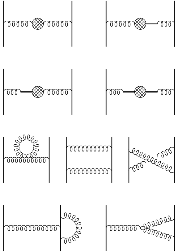
Figure 1: One loop topologies contributing to the static potential.

We now turn to the one loop corrections of (4.8). A representative set of topologies for this calculation is given in Figure $1$ where we have displayed the full set of corrections to the $2$-point functions. In those first four graphs the blob represents all the one loop corrections. However, due to the mixed propagator the correction to the $\xi^{ab}_{\mu}$ $2$-point function occurs even though there is no direct source $\xi^{ab}_{\mu}$ coupling. The two box diagrams are important for the exponentiation implied in the definition of the static potential, (4.4), and the asscociated issues with have been discussed at length in [48, 49, 50, 62, 63]. Therefore, it remains merely to compute the diagrams explicitly. Essential to this is the automatic Feynman diagram package Qgraf, [37], where the graphs are generated electronically and then converted into Form input notation. The algorithm we use is to break up all the Feynman graphs into simple master integrals and then identify the explicit functions for three dimensional spacetime. A comprehensive analysis of such masters to three loops are given in [39]. However, for our situation there are only two main integrals but there is the complication of having to work with a non-standard propagator which induces the canonical propagator to have a width after application of simple partial fractions, such as

$$\frac{p^{2}}{[(p^{2})^{2}+C_{A}\gamma^{4}]}~{}=~{}\frac{1}{2}\left[\frac{1}{[p^{2}+i\sqrt{C_{A}}\gamma^{2}]}~{}+~{}\frac{1}{2}\frac{1}{[p^{2}-i\sqrt{C_{A}}\gamma^{2}]}\right]$$ (4.12)

where now the momentum can involve the external momentum. In four dimensions the explicit expressions for Feynman integrals involved masses, $m$, and momenta, $p$, appearing in the form $m^{2}$ and $p^{2}$ respectively. However, in our three dimensional case with the drop in one unit of the dimensionality of the integral measure, the dependence is purely in terms of $m$ and $\sqrt{p^{2}}$. As discussed earlier for fields with a canonical mass term this is not a significant issue but when there is a width present one has to find the square root of the corresponding squared mass of the propagator. We follow the procedure used previously but allowing for the presence of the external momentum. Again ultimately one should obtain real and not complex expressions which is a check on our reasoning. So, for example, we have used the following intermediate expressions

$$\int_{k}\frac{1}{k^{2}[(k-p)^{2}+i\sqrt{C_{A}}\gamma^{2}]} = \frac{\sqrt{p^{2}}}{4\pi p^{2}}\tan^{-1}\left[\frac{\sqrt{p^{2}}}{\sqrt{i\sqrt{C_{A}}\gamma^{2}}}\right]$$

$$\int_{k}\frac{1}{[k^{2}+i\sqrt{C_{A}}\gamma^{2}][(k-p)^{2}+i\sqrt{C_{A}}\gamma^{2}]} = \frac{\sqrt{p^{2}}}{4\pi p^{2}}\tan^{-1}\left[\frac{\sqrt{p^{2}}}{2\sqrt{i\sqrt{C_{A}}\gamma^{2}}}\right]$$

$$\int_{k}\frac{1}{[k^{2}+i\sqrt{C_{A}}\gamma^{2}][(k-p)^{2}-i\sqrt{C_{A}}\gamma^{2}]} = \frac{\sqrt{p^{2}}}{4\pi p^{2}}\tan^{-1}\left[\frac{\sqrt{p^{2}}}{[\sqrt{i\sqrt{C_{A}}\gamma^{2}}+\sqrt{-i\sqrt{C_{A}}\gamma^{2}}}\right]$$ (4.13)

by adapting the results of [39] in the same way as before, where $\int_{k}$ $=$ $d^{d}k/(2\pi)^{d}$. In (4.13) we will use our simplification identities which allow us to write the functions of a complex variable in terms of a real and imaginary part. Although the three dimensional theory is finite, we still work in dimensional regularization with $d$ $=$ $3$ $-$ $2\epsilon$ as some of the master diagrams have poles in $\epsilon$, [39]. However, whilst the theory is ultraviolet finite we have been careful to check that there no (spurious) infrared infinities arise as a consequence of breaking the Feynman graphs up into scalar master integrals. For instance, such divergences could arise from the $1/p^{2}$ part of the propagators in the transverse projector or its powers but again we have checked that such potential terms cancel among themselves. This finiteness, at least to one loop, ensures that there is no source gluon renormalization constant as there is in the four dimensional arbitrary gauge calculation.

Given these considerations we are now in a position to record the one loop correction to (4.8) for (2.6). We find

$$\tilde{V}(\mathbf{p}) = -~{}\frac{C_{F}\mathbf{p}^{2}g^{2}}{[(\mathbf{p}^{2})^{2}+C_{A}\gamma^{4}]}$$ (4.14)

$$+~{}\left[\left[\frac{1}{2048}\eta_{1}(\mathbf{p}^{2})-\frac{1}{4096}\eta_{3}(\mathbf{p}^{2})\right]\frac{\sqrt{\mathbf{p}^{2}}}{\gamma^{4}}-\frac{\sqrt{2}C_{A}^{5/4}\gamma}{256[(\mathbf{p}^{2})^{2}+C_{A}\gamma^{4}]}-\frac{\sqrt{2}C_{A}^{5/4}\gamma}{4[(\mathbf{p}^{2})^{2}+16C_{A}\gamma^{4}]}\right.$$

$$\left.~{}~{}~{}~{}~{}+~{}\frac{\sqrt{2}C_{A}^{5/4}\gamma}{8[(\mathbf{p}^{2})^{2}-4C_{A}\gamma^{4}]}-\frac{\pi\sqrt{\mathbf{p}^{2}}T_{F}N_{\!f}C_{A}\gamma^{4}}{8[(\mathbf{p}^{2})^{2}+C_{A}\gamma^{4}]^{2}}\right.$$

$$\left.~{}~{}~{}~{}~{}+~{}\left[\frac{545}{2048}\eta_{1}(\mathbf{p}^{2})+\frac{515}{4096}\eta_{3}(\mathbf{p}^{2})\right]\frac{\sqrt{\mathbf{p}^{2}}C_{A}^{2}\gamma^{4}}{[(\mathbf{p}^{2})^{2}+C_{A}\gamma^{4}]^{2}}+\frac{49\pi\sqrt{\mathbf{p}^{2}}C_{A}^{2}\gamma^{4}}{1024[(\mathbf{p}^{2})^{2}+C_{A}\gamma^{4}]^{2}}\right.$$

$$\left.~{}~{}~{}~{}~{}-~{}\frac{13\sqrt{2}C_{A}^{9/4}\gamma^{5}}{384[(\mathbf{p}^{2})^{2}+C_{A}\gamma^{4}]^{2}}+\frac{\pi\sqrt{\mathbf{p}^{2}}T_{F}N_{\!f}}{8[(\mathbf{p}^{2})^{2}+C_{A}\gamma^{4}]}\right.$$

$$\left.~{}~{}~{}~{}~{}+~{}\left[\frac{11}{256}\eta_{2}(\mathbf{p}^{2})-\frac{313}{1024}\eta_{1}(\mathbf{p}^{2})-\frac{121}{2048}\eta_{3}(\mathbf{p}^{2})\right]\frac{\sqrt{\mathbf{p}^{2}}C_{A}}{[(\mathbf{p}^{2})^{2}+C_{A}\gamma^{4}]}\right.$$

$$\left.~{}~{}~{}~{}~{}-~{}\frac{49\pi\sqrt{\mathbf{p}^{2}}C_{A}}{1024[(\mathbf{p}^{2})^{2}+C_{A}\gamma^{4}]}-\frac{\sqrt{\mathbf{p}^{2}}C_{A}}{512(\mathbf{p}^{2})^{2}}\eta_{2}(\mathbf{p}^{2})\right.$$

$$\left.~{}~{}~{}~{}~{}-~{}\left[\frac{21}{1024}\eta_{4}(\mathbf{p}^{2})+\frac{3}{128}\eta_{5}(\mathbf{p}^{2})\right]\frac{\sqrt{C_{A}\mathbf{p}^{2}}}{\mathbf{p}^{2}\gamma^{2}}+\frac{\sqrt{2}C_{A}^{3/4}}{512\gamma\mathbf{p}^{2}}\right.$$

$$\left.~{}~{}~{}~{}~{}+~{}\left[\frac{11}{512}\eta_{4}(\mathbf{p}^{2})+\frac{47}{2048}\eta_{5}(\mathbf{p}^{2})\right]\frac{\sqrt{C_{A}}(\mathbf{p}^{2})^{3/2}}{[(\mathbf{p}^{2})^{2}+C_{A}\gamma^{4}]\gamma^{2}}-\frac{131\sqrt{2}C_{A}^{3/4}\mathbf{p}^{2}}{1024\gamma[(\mathbf{p}^{2})^{2}+C_{A}\gamma^{4}]}\right.$$

$$\left.~{}~{}~{}~{}~{}+~{}\frac{\sqrt{2}C_{A}^{3/4}\mathbf{p}^{2}}{16\gamma[(\mathbf{p}^{2})^{2}+16C_{A}\gamma^{4}]}+\frac{\sqrt{2}C_{A}^{3/4}\mathbf{p}^{2}}{16\gamma[(\mathbf{p}^{2})^{2}-4C_{A}\gamma^{4}]}-\frac{265C_{A}^{3/4}\gamma^{2}(\mathbf{p}^{2})^{3/2}}{2048[(\mathbf{p}^{2})^{2}+C_{A}\gamma^{4}]^{2}}\eta_{5}(\mathbf{p}^{2})\right.$$

$$\left.~{}~{}~{}~{}~{}+~{}\frac{121\sqrt{2}C_{A}^{7/4}\gamma^{3}\mathbf{p}^{2}}{3072[(\mathbf{p}^{2})^{2}+C_{A}\gamma^{4}]^{2}}\right]\frac{C_{F}g^{4}}{\pi}~{}+~{}O(g^{6})$$

where we have defined the intermediate functions $\eta_{i}(p^{2})$ by

$$\eta_{1}(p^{2}) = \tan^{-1}\left[\frac{\sqrt{2p^{2}}}{2C_{A}^{1/4}\gamma}\right]~{}~{}~{},~{}~{}~{}\eta_{2}(p^{2})~{}=~{}\tan^{-1}\left[\frac{\sqrt{2\sqrt{C_{A}}\gamma^{2}p^{2}}}{[\sqrt{C_{A}}\gamma^{2}-p^{2}]}\right]$$

$$\eta_{3}(p^{2}) = \tan^{-1}\left[\frac{2\sqrt{2\sqrt{C_{A}}\gamma^{2}p^{2}}}{[4\sqrt{C_{A}}\gamma^{2}-p^{2}]}\right]~{}~{}~{},~{}~{}~{}\eta_{4}(p^{2})~{}=~{}\ln\left[\frac{p^{2}+\sqrt{C_{A}}\gamma^{2}-\sqrt{2\sqrt{C_{A}}\gamma^{2}p^{2}}}{p^{2}+\sqrt{C_{A}}\gamma^{2}+\sqrt{2\sqrt{C_{A}}\gamma^{2}p^{2}}}\right]$$

$$\eta_{5}(p^{2}) = \ln\left[\frac{p^{2}+4\sqrt{C_{A}}\gamma^{2}-2\sqrt{2\sqrt{C_{A}}\gamma^{2}p^{2}}}{p^{2}+4\sqrt{C_{A}}\gamma^{2}+2\sqrt{2\sqrt{C_{A}}\gamma^{2}p^{2}}}\right]~{}.$$ (4.15)

Essentially these arise from taking the real and imaginary parts of expressions such as those given in (4.13).

As a check on (4.14) if we take the $\gamma$ $\rightarrow$ $0$ limit we recover the one loop expression of [53, 61] given in (4.1). We stress though that whilst (4.1) was computed in an arbitrary linear covariant gauge we have been restricted to the Landau gauge as we have incorporated the Gribov problem within the Lagrangian. However, (4.14) represents the first non-trivial check on (4.1). Given that (2.6) is supposed to represent a confining theory we can now examine (4.14) to see if the dominant behaviour in the zero momentum limit could deliver a behaviour leading to a linearly rising potential. In three dimensions this would correspond to an $O(\sqrt{p^{2}}/(p^{2})^{2})$ type term and in (4.14) there is one term which appears with such a singularity. However, its numerator involves the function $\eta_{2}(p^{2})$ which vanishes at zero momentum and therefore, the appropriate singular behaviour does not seem to emerge. More concretely as $p^{2}$ $\rightarrow$ $0$ we have

$$\tilde{V}(\mathbf{p})~{}=~{}-~{}\frac{C_{F}\mathbf{p}^{2}g^{2}}{C_{A}\gamma^{4}}~{}-~{}C_{F}\left[\frac{\sqrt{2}C_{A}^{1/4}}{48\gamma^{3}}~{}+~{}\frac{113\sqrt{2}\mathbf{p}^{2}}{1920\pi C_{A}^{1/4}\gamma^{5}}\right]g^{4}~{}+~{}O((\mathbf{p}^{2})^{2};g^{6})~{}.$$ (4.16)

Therefore, similar to the four dimensional case, [25], the one loop correction freezes to a finite value, which is

$$\tilde{V}(0)~{}=~{}-~{}\frac{\sqrt{2}C_{F}C_{A}^{1/4}g^{4}}{48\pi\gamma^{3}}~{}+~{}O(g^{6})$$ (4.17)

and there is no net divergence whose presence would at least be necessary for a rising potential. There is a degree of irony with this observation in that the $\gamma$ $=$ $0$ potential at one loop has a Fourier transform which produces a linearly rising potential. Though in that case in is not clear what would transpire at two loops given the dimensionality of the coupling constant. However, as noted in [24, 25] the more appropriate route to proceed down would be to analyse the zero momentum behaviour of the propagators of the localizing fields. Whilst the fermionic ghosts are both enhanced at zero momentum in (2.6), it has recently been shown that the same is true for certain colour components of the Bose ghost, [24, 25]. This property is independent of the spacetime dimension, [25], but it has not been fully determined what the implications are for the static potential.

5 Formal propagator corrections.

We turn now to the enhancement of the Bose ghost fields. Recently the structure of these fields was analysed non-perturbatively by Zwanziger in [24] where it was demonstrated that there was enhancement in certain colour channels. The result is based on the spontaneous breaking of the BRST symmetry but given the presence of the horizon condition, which equates to a constraint on the gluon and $\xi^{ab}_{\mu}$ fields, this requires a more careful analysis than usual. One key outcome is that the associated Goldstone bosons of this spontaneous breaking generate massless excitations non-perturbatively but crucially in the context of the Gribov-Zwanziger Lagrangian, these fields are enhanced in the infrared. One consequence is that this enhancement is present order by order in perturbation theory and this was confirmed by explicit one loop calculations in four dimensions in the $\overline{\mbox{MS}}$ scheme, [25]. However, in [25] the main emphasis was on the transverse part of the propagators since the interest was in examining the implications for the static potential for heavy coloured objects. The longitudinal piece of the exchanged particle does not contribute in the particular configuration considered for the Wilson loop. In this section we provide the formal construction of the full propagator for the gluon and $\xi^{ab}_{\mu}$ fields prior to considering the behaviour in the infrared limit when the gap equation is realised which is given specifically in the next section. Although we concentrate primarily on three dimensions in this article we will also include the analysis for four dimensions in this section. This is because the general reasoning of [24] is dimension independent and we confirm this at one loop by considering both dimensions within our analysis here.

We begin by recalling how enhancement occurs for the simple situation of the Faddeev-Popov ghost, $c^{a}$. As was demonstrated in Gribov’s seminal contribution, [5], one computes the ghost $2$-point function at one loop when the horizon condition is implemented in the path integral. The consequent presence of the Gribov mass in the gluon propagator produces an expression which differs from what one would obtain using a canonical propagator. Expanding the finite function of the momentum in a Taylor series around zero momentum it transpires that the leading term is equivalent to the one loop correction to the Gribov mass gap equation. As the theory has no meaning as a gauge theory unless $\gamma$ satisfies the gap equation, this implies that the leading term of the $2$-point function in this limit is not $O(p^{2})$ but $O\left((p^{2})^{2}\right)$. Hence, the low energy behaviour of Faddeev-Popov ghost propagator is not the usual perturbative form but the enhanced dipole form. Subsequently, this property of ghost enhancement has been translated into the Kugo-Ojima confinement condition. This was originally established in [12, 13] for the Landau gauge version of Yang-Mills involving only Faddeev-Popov ghosts. More recently the criterion has been extended to the Gribov-Zwanziger context where there are additional fermionic ghosts, $\omega^{ab}_{\mu}$, which are clearly absent in the original Kugo-Ojima BRST analysis, as well as the Bose ghosts, $\rho^{ab}_{\mu}$ and $\xi^{ab}_{\mu}$, [14]. In the context of (2.6) it has now been established that $\omega^{ab}_{\mu}$ also enhances. It has been demonstrated in the full analysis of [24, 36] and in explicit two loop $\overline{\mbox{MS}}$ computations in four dimensions, [23]. We note at this point that we have repeated the latter calculations for $\omega^{ab}_{\mu}$ in the three dimensional version of (2.6) and have verified that when $\gamma$ satisfies the two loop gap equation, (3.8), the fermionic ghost enhances.

In focusing on the Faddeev-Popov enhancement derivation the key ingredient is the zero momentum limit of the $2$-point functions. As we have evaluated the $2$-point function corrections exactly at one loop for all the fields we can now consider the situation for the Bose ghost fields. For ease we consider the $\rho^{ab}_{\mu}$ field first. In the zero momentum limit we have,

$$\langle\rho^{ab}_{\mu}(p)\rho^{cd}_{\nu}(-p)\rangle^{-1}~{}=~{}-~{}\delta^{ac}\delta^{bd}\eta_{\mu\nu}\left[1~{}-~{}\frac{\sqrt{2}C_{A}^{3/4}g^{2}}{12\pi\gamma}~{}+~{}\frac{\sqrt{2}C_{A}^{1/4}g^{2}}{60\pi\gamma^{3}}p^{2}~{}+~{}O\left((p^{2})^{2}\right)\right]p^{2}~{}+~{}O(g^{4})$$ (5.1)

whence it is elementary to observe that the leading one loop correction is precisely that which appears in the gap equation, (3.8). Hence, when $\gamma$ fulfils that condition the leading term of the $2$-point function is the $O\left((p^{2})^{2}\right)$ part of the one loop term. Consequently when one inverts the coefficient of the $\eta_{\mu\nu}$ tensor in this zero momentum limit then the $\rho^{ab}_{\mu}$ field enhances. One could, of course, consider the transverse and longitudinal parts of (5.1) separately which is how the $A^{a}_{\mu}$ and $\xi^{ab}_{\mu}$ system was considered in [25]. However, the upshot is that the $\rho^{ab}_{\mu}$ propagator at low momentum is

$$\langle\rho^{ab}_{\mu}(p)\rho^{cd}_{\nu}(-p)\rangle~{}\sim~{}-~{}\frac{30\sqrt{2}\pi\gamma^{3}}{C_{A}^{1/4}(p^{2})^{2}g^{2}}\delta^{ac}\delta^{bd}\eta_{\mu\nu}~{}.$$ (5.2)

Although the explicit expressions for the two loop corrections to the $2$-point functions are not available, it is possible to determine their zero momentum behaviour using the vacuum bubble expansion. A similar procedure was followed in the four dimensional case and we note that at two loops the leading momentum part of the $\rho^{ab}_{\mu}$ $2$-point function is precisely the two loop gap equation (3.8). Therefore, the enhancement of $\rho^{ab}_{\mu}$ is present at next order in exact agreement with the general BRST arguments of [24].

Whilst this demonstrates that a part of the Bose ghost can enhance we need to complete the analysis by considering the imaginary component which is more involved due to it being entwined with $A^{a}_{\mu}$. In three dimensions the zero momentum limit of the $2$-point function is

$$\langle\xi^{ab}_{\mu}(p)\xi^{cd}_{\nu}(-p)\rangle^{-1} = -~{}\left[\delta^{ac}\delta^{bd}\left[1~{}-~{}\frac{\sqrt{2}C_{A}^{3/4}g^{2}}{12\pi\gamma}\right]p^{2}~{}+~{}\frac{7\sqrt{2}g^{2}}{2880\pi C_{A}^{1/4}\gamma}f^{ace}f^{bde}p^{2}\right.$$ (5.3)

$$\left.~{}~{}~{}~{}+~{}\frac{\sqrt{2}g^{2}}{720\pi C_{A}^{1/4}\gamma}f^{abe}f^{cde}p^{2}~{}+~{}\frac{7\sqrt{2}g^{2}}{480\pi C_{A}^{5/4}\gamma}d_{A}^{abcd}p^{2}~{}+~{}O(g^{4})\right]P_{\mu\nu}(p)$$

$$-~{}\left[\delta^{ac}\delta^{bd}\left[1~{}-~{}\frac{\sqrt{2}C_{A}^{3/4}g^{2}}{12\pi\gamma}\right]p^{2}~{}+~{}\frac{\sqrt{2}g^{2}}{180\pi C_{A}^{1/4}\gamma}f^{ace}f^{bde}p^{2}\right.$$

$$\left.~{}~{}~{}~{}-~{}\frac{\sqrt{2}g^{2}}{360\pi C_{A}^{1/4}\gamma}f^{abe}f^{cde}p^{2}~{}+~{}\frac{\sqrt{2}g^{2}}{30\pi C_{A}^{5/4}\gamma}d_{A}^{abcd}p^{2}~{}+~{}O(g^{4})\right]L_{\mu\nu}(p)$$

$$+~{}O\left((p^{2})^{2}\right)~{}.$$

Clearly the piece analogous to (5.1) would equate to enhancement if one could perform the zero momentum inversion of (5.3) in the absence of the additional colour channels. However, not only would this not be correct it would ignore the fact that the construction of the propagators actually requires $A^{a}_{\mu}$ to be included due to the mixed quadratic term of (2.6). In order to do this we consider the problem of the inversion in a general context. First, we recall the procedure for the transverse sector, [25], and define the matrix of colour amplitudes of the $2$-point functions of the set of fields $\{A^{a}_{\mu},\xi^{ab}_{\mu},\rho^{ab}_{\mu}\}$ by

$$\Lambda^{\{ab|cd\}}~{}=~{}\left(\begin{array}[]{ccc}{\cal X}\delta^{ac}&{\cal U}f^{acd}&0\\ {\cal U}f^{cab}&{\cal Q}^{abcd}_{\xi}&0\\ 0&0&{\cal Q}^{abcd}_{\rho}\\ \end{array}\right)$$ (5.4)

where

$${\cal Q}^{abcd}_{\xi} = {\cal Q}_{\xi}\delta^{ac}\delta^{bd}~{}+~{}{\cal W}_{\xi}f^{ace}f^{bde}~{}+~{}{\cal R}_{\xi}f^{abe}f^{cde}~{}+~{}{\cal S}_{\xi}d_{A}^{abcd}~{}+~{}{\cal P}_{\xi}\delta^{ab}\delta^{cd}~{}+~{}{\cal T}_{\xi}\delta^{ad}\delta^{bc}$$

$${\cal Q}^{abcd}_{\rho} = {\cal Q}_{\rho}\delta^{ac}\delta^{bd}~{}+~{}{\cal W}_{\rho}f^{ace}f^{bde}~{}+~{}{\cal R}_{\rho}f^{abe}f^{cde}~{}+~{}{\cal S}_{\rho}d_{A}^{abcd}~{}+~{}{\cal P}_{\rho}\delta^{ab}\delta^{cd}~{}+~{}{\cal T}_{\rho}\delta^{ad}\delta^{bc}$$

and, [64],

$$d_{A}^{abcd}~{}=~{}\frac{1}{6}\mbox{Tr}\left(T_{A}^{a}T_{A}^{(b}T_{A}^{c}T_{A}^{d)}\right)$$ (5.6)

is totally symmetric. The subscript on the group generator $T_{A}^{a}$ indicates that it is in the adjoint representation. We have omitted the common transverse projector from (5.4). Including $\rho^{ab}_{\mu}$ in the basis here may not appear to be necessary since (5.4) is block diagonal, and we have treated it already, but it is relevant when we examine the longitudinal sector since not all the corresponding zero entries of (5.4) remain zero. In introducing general amplitudes for the colour decomposition we note that each represents the leading term of the $2$-point function as well as the loop corrections. In each of the rank four colour decompositions we have included structures which do not arise in the explicit computations at one loop. Aside from ensuring we work with a complete basis such structures may occur at a higher loop order but they will also give us an insight into the effect such pieces have on the form of the inverse of the matrix which is the propagators. For this we formally define the inverse in a similar way with

$$\Pi^{\{cd|pq\}}~{}=~{}\left(\begin{array}[]{ccc}{\cal A}\delta^{cp}&{\cal B}f^{cpq}&0\\ {\cal B}f^{pcd}&{\cal D}^{cdpq}_{\xi}&0\\ 0&0&{\cal D}^{cdpq}_{\rho}\\ \end{array}\right)$$ (5.7)

where

$${\cal D}^{cdpq}_{\xi} = {\cal D}_{\xi}\delta^{cp}\delta^{dq}~{}+~{}{\cal J}_{\xi}f^{cpe}f^{dqe}~{}+~{}{\cal K}_{\xi}f^{cde}f^{pqe}~{}+~{}{\cal L}_{\xi}d_{A}^{cdpq}~{}+~{}{\cal M}_{\xi}\delta^{cd}\delta^{pq}~{}+~{}{\cal N}_{\xi}\delta^{cq}\delta^{dp}$$

$${\cal D}^{cdpq}_{\rho} = {\cal D}_{\rho}\delta^{cp}\delta^{dq}~{}+~{}{\cal J}_{\rho}f^{cpe}f^{dqe}~{}+~{}{\cal K}_{\rho}f^{cde}f^{pqe}~{}+~{}{\cal L}_{\rho}d_{A}^{cdpq}~{}+~{}{\cal M}_{\rho}\delta^{cd}\delta^{pq}~{}+~{}{\cal N}_{\rho}\delta^{cq}\delta^{dp}$$

and the transverse projector is again omitted. As $\Pi^{\{ab|cd\}}$ is the inverse colour matrix, it satisfies

$$\Lambda^{\{ab|cd\}}\Pi^{\{cd|pq\}}~{}=~{}\left(\begin{array}[]{ccc}\delta^{cp}&0&0\\ 0&\delta^{cp}\delta^{dq}&0\\ 0&0&\delta^{cp}\delta^{dq}\\ \end{array}\right)$$ (5.9)

where the right hand side is the unit matrix in the colour vector space of the basis of fields we use. For the inversion relating to the Lorentz structure, we recall the trivial identity

$$\eta_{\mu\nu}~{}=~{}P_{\mu\nu}(p)~{}+~{}L_{\mu\nu}(p)$$ (5.10)

and note that the first term on the right side is where our current focus is.

The method to find the formal inverse is to multiply out the matrices and solve the resulting relations between the amplitudes algebraically. In order to do this we note that the products involving $d_{A}^{abcd}$ can be simplified with the relations, [25],

$$d_{A}^{abpq}d_{A}^{cdpq} = a_{1}\delta^{ab}\delta^{cd}~{}+~{}a_{2}\left(\delta^{ac}\delta^{bd}~{}+~{}\delta^{ad}\delta^{bc}\right)~{}+~{}a_{3}\left(f^{ace}f^{bde}~{}+~{}f^{ade}f^{bce}\right)~{}+~{}a_{4}d_{A}^{abcd}$$

$$f^{ape}f^{bqe}d_{A}^{cdpq} = b_{1}\delta^{ab}\delta^{cd}~{}+~{}b_{2}\left(\delta^{ac}\delta^{bd}~{}+~{}\delta^{ad}\delta^{bc}\right)$$ (5.11)

$$+~{}b_{3}\left(f^{ace}f^{bde}~{}+~{}f^{ade}f^{bce}\right)~{}+~{}b_{4}d_{A}^{abcd}$$

where the coefficients are defined by, [25],

$$a_{1} = -~{}\left[540C_{A}^{2}N_{\!A}(N_{\!A}-3)d_{A}^{abcd}d_{A}^{cdpq}d_{A}^{abpq}+144(2N_{\!A}+19)\left(d_{A}^{abcd}d_{A}^{abcd}\right)^{2}\right.$$

$$\left.~{}~{}~{}~{}-~{}150C_{A}^{4}N_{\!A}(3N_{\!A}+11)d_{A}^{abcd}d_{A}^{abcd}+625C_{A}^{8}N_{\!A}^{2}\right]$$

$$~{}~{}~{}\times~{}\frac{1}{54N_{\!A}(N_{\!A}-3)[12(N_{\!A}+2)d_{A}^{efgh}d_{A}^{efgh}-25C_{A}^{4}N_{\!A}]}$$

$$a_{2} = \left[144(11N_{\!A}-8)\left(d_{A}^{abcd}d_{A}^{abcd}\right)^{2}\right.-1080C_{A}^{2}N_{\!A}(N_{\!A}-3)d_{A}^{abcd}d_{A}^{cdpq}d_{A}^{abpq}$$

$$\left.~{}+~{}625C_{A}^{8}N_{\!A}^{2}-3000C_{A}^{4}N_{\!A}d_{A}^{abcd}d_{A}^{abcd}\right]$$

$$\times~{}\frac{1}{108N_{\!A}(N_{\!A}-3)[12(N_{\!A}+2)d_{A}^{efgh}d_{A}^{efgh}-25C_{A}^{4}N_{\!A}]}$$

$$a_{3} = \frac{[12(N_{\!A}+2)d_{A}^{abcd}d_{A}^{abcd}-25C_{A}^{4}N_{\!A}]}{54C_{A}N_{\!A}(N_{\!A}-3)}$$

$$a_{4} = \frac{[216(N_{\!A}+2)d_{A}^{abcd}d_{A}^{cdpq}d_{A}^{abpq}-125C_{A}^{6}N_{\!A}-360C_{A}^{2}d_{A}^{abcd}d_{A}^{abcd}]}{18[12(N_{\!A}+2)d_{A}^{efgh}d_{A}^{efgh}-25C_{A}^{4}N_{\!A}]}$$ (5.12)

and

$$b_{1}~{}=~{}-~{}2b_{2}~{}=~{}\frac{[5C_{A}^{4}N_{\!A}-12d_{A}^{abcd}d_{A}^{abcd}]}{9C_{A}N_{\!A}(N_{\!A}-3)}~{}~{},~{}~{}b_{3}~{}=~{}\frac{[6(N_{\!A}-1)d_{A}^{abcd}d_{A}^{abcd}-5C_{A}^{4}N_{\!A}]}{9C_{A}^{2}N_{\!A}(N_{\!A}-3)}~{}~{},~{}~{}b_{4}~{}=~{}\frac{C_{A}}{3}~{}.$$ (5.13)

Multiplying out the matrices results in the relations

$$1 = {\cal AX}~{}+~{}C_{A}{\cal UB}~{}~{}~{},~{}~{}~{}0~{}=~{}{\cal XB}~{}+~{}\left({\cal D}_{\xi}-{\cal N}_{\xi}+C_{A}{\cal K}_{\xi}+\frac{1}{2}C_{A}{\cal J}_{\xi}\right){\cal U}$$

$$0 = {\cal A}{\cal U}~{}+~{}\left({\cal Q}_{\xi}+C_{A}{\cal R}_{\xi}+\frac{1}{2}C_{A}{\cal W}_{\xi}-{\cal T}_{\xi}\right){\cal B}$$

$$1 = {\cal Q}_{\xi}{\cal D}_{\xi}~{}+~{}b_{2}{\cal L}_{\xi}{\cal W}_{\xi}~{}+~{}b_{2}{\cal S}_{\xi}{\cal J}_{\xi}~{}+~{}a_{2}{\cal S}_{\xi}{\cal L}_{\xi}~{}+~{}{\cal T}_{\xi}{\cal N}_{\xi}$$

$$0 = \left({\cal Q}_{\xi}+C_{A}{\cal W}_{\xi}+\frac{5}{6}C_{A}^{2}{\cal S}_{\xi}+N_{\!A}{\cal P}_{\xi}+{\cal T}_{\xi}\right){\cal M}_{\xi}~{}+~{}\left(C_{A}{\cal J}_{\xi}+\frac{5}{6}C_{A}^{2}{\cal L}_{\xi}+{\cal D}_{\xi}+{\cal N}_{\xi}\right){\cal P}_{\xi}$$

$$+~{}b_{1}{\cal W}_{\xi}{\cal L}_{\xi}~{}+~{}b_{1}{\cal S}_{\xi}{\cal J}_{\xi}~{}+~{}a_{1}{\cal S}_{\xi}{\cal L}_{\xi}$$

$$0 = b_{2}{\cal L}_{\xi}{\cal W}_{\xi}~{}+~{}b_{2}{\cal S}_{\xi}{\cal J}_{\xi}~{}+~{}a_{2}{\cal S}_{\xi}{\cal L}_{\xi}~{}+~{}{\cal Q}_{\xi}{\cal N}_{\xi}~{}+~{}{\cal T}_{\xi}{\cal D}_{\xi}$$

$$0 = {\cal Q}_{\xi}{\cal L}_{\xi}~{}+~{}{\cal W}_{\xi}{\cal J}_{\xi}~{}+~{}{\cal S}_{\xi}{\cal D}_{\xi}~{}+~{}b_{4}{\cal W}_{\xi}{\cal L}_{\xi}~{}+~{}b_{4}{\cal S}_{\xi}{\cal J}_{\xi}~{}+~{}a_{4}{\cal S}_{\xi}{\cal L}_{\xi}~{}+~{}{\cal S}_{\xi}{\cal N}_{\xi}~{}+~{}{\cal T}_{\xi}{\cal L}_{\xi}$$

$$0 = {\cal W}_{\xi}{\cal D}_{\xi}~{}+~{}{\cal Q}_{\xi}{\cal J}_{\xi}~{}+~{}\frac{1}{6}C_{A}{\cal W}_{\xi}{\cal J}_{\xi}~{}+~{}2b_{3}{\cal S}_{\xi}{\cal J}_{\xi}~{}+~{}2a_{3}{\cal S}_{\xi}{\cal L}_{\xi}~{}+~{}2b_{3}{\cal W}_{\xi}{\cal L}_{\xi}~{}+~{}{\cal W}_{\xi}{\cal N}_{\xi}~{}+~{}{\cal T}_{\xi}{\cal J}_{\xi}$$

$$0 = {\cal UB}~{}+~{}{\cal Q}_{\xi}{\cal K}_{\xi}~{}+~{}\frac{1}{6}C_{A}{\cal W}_{\xi}{\cal J}_{\xi}~{}+~{}\frac{1}{2}C_{A}{\cal W}_{\xi}{\cal K}_{\xi}~{}+~{}\frac{1}{2}C_{A}{\cal R}_{\xi}{\cal J}_{\xi}~{}+~{}C_{A}{\cal R}_{\xi}{\cal K}_{\xi}~{}-~{}b_{3}{\cal W}_{\xi}{\cal L}_{\xi}$$ (5.14)

$$-~{}{\cal W}_{\xi}{\cal N}_{\xi}~{}+~{}{\cal R}_{\xi}{\cal D}_{\xi}~{}-~{}{\cal R}_{\xi}{\cal N}_{\xi}~{}-~{}b_{3}{\cal S}_{\xi}{\cal J}_{\xi}~{}-~{}a_{3}{\cal S}_{\xi}{\cal L}_{\xi}~{}-~{}{\cal T}_{\xi}{\cal J}_{\xi}~{}-~{}{\cal T}_{\xi}{\cal K}_{\xi}$$

for the $A^{a}_{\mu}$ and $\xi^{ab}_{\mu}$ sector. The full set for the $\rho^{ab}_{\mu}$ sector is

$$1 = {\cal Q}_{\rho}{\cal D}_{\rho}~{}+~{}b_{2}{\cal L}_{\rho}{\cal W}_{\rho}~{}+~{}b_{2}{\cal S}_{\rho}{\cal J}_{\rho}~{}+~{}a_{2}{\cal S}_{\rho}{\cal L}_{\rho}~{}+~{}{\cal T}_{\rho}{\cal N}_{\rho}$$

$$0 = \left({\cal Q}_{\rho}+C_{A}{\cal W}_{\rho}+\frac{5}{6}C_{A}^{2}{\cal S}_{\rho}+N_{\!A}{\cal P}_{\rho}+{\cal T}_{\rho}\right){\cal M}_{\rho}~{}+~{}\left(C_{A}{\cal J}_{\rho}+\frac{5}{6}C_{A}^{2}{\cal L}_{\rho}+{\cal D}_{\rho}+{\cal N}_{\rho}\right){\cal P}_{\rho}$$

$$+~{}b_{1}{\cal W}_{\rho}{\cal L}_{\rho}~{}+~{}b_{1}{\cal S}_{\rho}{\cal J}_{\rho}~{}+~{}a_{1}{\cal S}_{\rho}{\cal L}_{\rho}$$

$$0 = b_{2}{\cal L}_{\rho}{\cal W}_{\rho}~{}+~{}b_{2}{\cal S}_{\rho}{\cal J}_{\rho}~{}+~{}a_{2}{\cal S}_{\rho}{\cal L}_{\rho}~{}+~{}{\cal Q}_{\rho}{\cal N}_{\rho}~{}+~{}{\cal T}_{\rho}{\cal D}_{\rho}$$

$$0 = {\cal Q}_{\rho}{\cal L}_{\rho}~{}+~{}{\cal W}_{\rho}{\cal J}_{\rho}~{}+~{}{\cal S}_{\rho}{\cal D}_{\rho}~{}+~{}b_{4}{\cal W}_{\rho}{\cal L}_{\rho}~{}+~{}b_{4}{\cal S}_{\rho}{\cal J}_{\rho}~{}+~{}a_{4}{\cal S}_{\rho}{\cal L}_{\rho}~{}+~{}{\cal S}_{\rho}{\cal N}_{\rho}~{}+~{}{\cal T}_{\rho}{\cal L}_{\rho}$$

$$0 = {\cal W}_{\rho}{\cal D}_{\rho}~{}+~{}{\cal Q}_{\rho}{\cal J}_{\rho}~{}+~{}\frac{1}{6}C_{A}{\cal W}_{\rho}{\cal J}_{\rho}~{}+~{}2b_{3}{\cal S}_{\rho}{\cal J}_{\rho}$$

$$+~{}2a_{3}{\cal S}_{\rho}{\cal L}_{\rho}~{}+~{}2b_{3}{\cal W}_{\rho}{\cal L}_{\rho}~{}+~{}{\cal W}_{\rho}{\cal N}_{\rho}~{}+~{}{\cal T}_{\rho}{\cal J}_{\rho}$$

$$0 = {\cal Q}_{\rho}{\cal K}_{\rho}~{}+~{}\frac{1}{6}C_{A}{\cal W}_{\rho}{\cal J}_{\rho}~{}+~{}\frac{1}{2}C_{A}{\cal W}_{\rho}{\cal K}_{\rho}~{}+~{}\frac{1}{2}C_{A}{\cal R}_{\rho}{\cal J}_{\rho}~{}+~{}C_{A}{\cal R}_{\rho}{\cal K}_{\rho}~{}-~{}b_{3}{\cal W}_{\rho}{\cal L}_{\rho}$$ (5.15)

$$-~{}{\cal W}_{\rho}{\cal N}_{\rho}~{}+~{}{\cal R}_{\rho}{\cal D}_{\rho}~{}-~{}{\cal R}_{\rho}{\cal N}_{\rho}~{}-~{}b_{3}{\cal S}_{\rho}{\cal J}_{\rho}~{}-~{}a_{3}{\cal S}_{\rho}{\cal L}_{\rho}~{}-~{}{\cal T}_{\rho}{\cal J}_{\rho}~{}-~{}{\cal T}_{\rho}{\cal K}_{\rho}~{}.$$

Whilst this set appears formally similar to the corresponding equations of the $A^{a}_{\mu}$ and $\xi^{ab}_{\mu}$ subset, the final equation has one fewer term.

For an arbitrary colour group the full solution to both sets of equations are cumbersome. For instance, by way of illustration for the slightly simpler case of the $\rho^{ab}_{\mu}$ sector we have recorded the full expressions for $SU(N_{c})$ in Appendix C. For the top sector the gluon and mixed propagators are simple for an arbitrary colour group giving

$${\cal A} = \frac{[{\cal Q}_{\xi}+C_{A}{\cal R}_{\xi}+\mbox{\small{$\frac{1}{2}$}}C_{A}{\cal W}_{\xi}]}{[({\cal Q}_{\xi}+C_{A}{\cal R}_{\xi}+\mbox{\small{$\frac{1}{2}$}}C_{A}{\cal W}_{\xi}){\cal X}-C_{A}{\cal U}^{2}]}$$

$${\cal B} = -~{}\frac{{\cal U}}{[({\cal Q}_{\xi}+C_{A}{\cal R}_{\xi}+\mbox{\small{$\frac{1}{2}$}}C_{A}{\cal W}_{\xi}){\cal X}-C_{A}{\cal U}^{2}]}~{}.$$ (5.16)

However, for the $\xi^{ab}_{\mu}$ propagator we only present the expressions for $SU(3)$ which are

$${\cal D}_{\xi} = \frac{1}{2{\cal Q}_{\xi}}\left[3(3{\cal S}_{\xi}-2{\cal W}_{\xi})({\cal S}_{\xi}+2{\cal W}_{\xi})({\cal S}_{\xi}+{\cal W}_{\xi})+8(7{\cal S}_{\xi}+3{\cal W}_{\xi}){\cal Q}_{\xi}^{2}\right.$$

$$\left.~{}~{}~{}~{}~{}+~{}16{\cal Q}_{\xi}^{3}+2(27{\cal S}_{\xi}^{3}+20{\cal S}_{\xi}{\cal W}_{\xi}-8{\cal W}_{\xi}^{2}){\cal Q}_{\xi}\right]$$

$$~{}\times\left[2{\cal Q}_{\xi}+3{\cal S}_{\xi}+3{\cal W}_{\xi}\right]^{-1}\left[2{\cal Q}_{\xi}+3{\cal S}_{\xi}-2{\cal W}_{\xi}\right]^{-1}\left[2{\cal Q}_{\xi}+{\cal S}_{\xi}+2{\cal W}_{\xi}\right]^{-1}$$

$${\cal J}_{\xi} = -~{}\frac{4{\cal W}_{\xi}}{[2{\cal Q}_{\xi}+3{\cal S}_{\xi}+3{\cal W}_{\xi}][2{\cal Q}_{\xi}+3{\cal S}_{\xi}-2{\cal W}_{\xi}]}$$

$${\cal K}_{\xi} = \frac{1}{{\cal Q}_{\xi}}\left[(4(3{\cal S}_{\xi}-{\cal W}_{\xi}){\cal Q}_{\xi}+3(3{\cal S}_{\xi}-2{\cal W}_{\xi})({\cal S}_{\xi}+{\cal W}_{\xi}))(2{\cal U}^{2}-{\cal W}_{\xi}{\cal X}-2{\cal R}_{\xi}{\cal X})\right.$$

$$\left.~{}~{}~{}~{}-~{}8({\cal R}_{\xi}{\cal X}-{\cal U})^{2}{\cal Q}_{\xi}^{2}\right]$$

$$~{}\times\left[2{\cal Q}_{\xi}{\cal X}+6{\cal R}_{\xi}{\cal X}-6{\cal U}^{2}+3{\cal W}_{\xi}{\cal X}\right]^{-1}\left[2{\cal Q}_{\xi}+3{\cal S}_{\xi}+3{\cal W}_{\xi}\right]^{-1}\left[2{\cal Q}_{\xi}+3{\cal S}_{\xi}-2{\cal W}_{\xi}\right]^{-1}$$

$${\cal L}_{\xi} = -~{}4\left[2{\cal Q}_{\xi}{\cal S}_{\xi}+(3{\cal S}_{\xi}+2{\cal W}_{\xi})({\cal S}_{\xi}-{\cal W}_{\xi})\right]$$

$$~{}~{}\times\left[2{\cal Q}_{\xi}+3{\cal S}_{\xi}+3{\cal W}_{\xi}\right]^{-1}\left[2{\cal Q}_{\xi}+3{\cal S}_{\xi}-2{\cal W}_{\xi}\right]^{-1}\left[2{\cal Q}_{\xi}+{\cal S}_{\xi}+2{\cal W}_{\xi}\right]^{-1}$$

$${\cal M}_{\xi} = 6\left[21{\cal S}_{\xi}^{3}+{\cal S}_{\xi}^{2}{\cal W}_{\xi}-12{\cal S}_{\xi}{\cal W}_{\xi}^{2}-4{\cal W}_{\xi}^{3}+2(7{\cal S}_{\xi}+4{\cal W}_{\xi}){\cal Q}_{\xi}{\cal S}_{\xi}\right]\left[2{\cal Q}_{\xi}+15{\cal S}_{\xi}+6{\cal W}_{\xi}\right]^{-1}$$

$$\times\left[2{\cal Q}_{\xi}+3{\cal S}_{\xi}+3{\cal W}_{\xi}\right]^{-1}\left[2{\cal Q}_{\xi}+3{\cal S}_{\xi}-2{\cal W}_{\xi}\right]^{-1}\left[2{\cal Q}_{\xi}+{\cal S}_{\xi}+2{\cal W}_{\xi}\right]^{-1}$$

$${\cal N}_{\xi} = -~{}\frac{3}{2{\cal Q}_{\xi}}\left[(3{\cal S}_{\xi}-2{\cal W}_{\xi})({\cal S}_{\xi}+2{\cal W}_{\xi})({\cal S}_{\xi}+{\cal W}_{\xi})+2({\cal S}_{\xi}+4{\cal W}_{\xi}){\cal Q}_{\xi}{\cal S}_{\xi}\right]$$ (5.17)

$$~{}~{}~{}\times\left[2{\cal Q}_{\xi}+3{\cal S}_{\xi}+3{\cal W}_{\xi}\right]^{-1}\left[2{\cal Q}_{\xi}+3{\cal S}_{\xi}-2{\cal W}_{\xi}\right]^{-1}\left[2{\cal Q}_{\xi}+{\cal S}_{\xi}+2{\cal W}_{\xi}\right]^{-1}~{}.$$

Next we formally repeat the procedure for the longitudinal part of the matrix of $2$-point functions and denote the corresponding quantities with a superscript ^L. For instance, the matrix of $2$-point functions is now

$$\Lambda^{L\,\{ab|cd\}}~{}=~{}\left(\begin{array}[]{ccc}{\cal X}^{L}\delta^{ac}&{\cal U}^{L}f^{acd}&{\cal V}^{L}f^{acd}\\ {\cal U}^{L}f^{cab}&{\cal Q}^{L\,abcd}_{\xi}&0\\ {\cal V}^{L}f^{cab}&0&{\cal Q}^{L\,abcd}_{\rho}\\ \end{array}\right)$$ (5.18)

where

$${\cal Q}^{L\,abcd}_{\xi} = {\cal Q}^{L}_{\xi}\delta^{ac}\delta^{bd}~{}+~{}{\cal W}^{L}_{\xi}f^{ace}f^{bde}~{}+~{}{\cal R}^{L}_{\xi}f^{abe}f^{cde}~{}+~{}{\cal S}^{L}_{\xi}d_{A}^{abcd}~{}+~{}{\cal P}^{L}_{\xi}\delta^{ab}\delta^{cd}~{}+~{}{\cal T}^{L}_{\xi}\delta^{ad}\delta^{bc}$$

$${\cal Q}^{L\,abcd}_{\rho} = {\cal Q}^{L}_{\rho}\delta^{ac}\delta^{bd}~{}+~{}{\cal W}^{L}_{\rho}f^{ace}f^{bde}~{}+~{}{\cal R}^{L}_{\rho}f^{abe}f^{cde}~{}+~{}{\cal S}^{L}_{\rho}d_{A}^{abcd}~{}+~{}{\cal P}^{L}_{\rho}\delta^{ab}\delta^{cd}~{}+~{}{\cal T}^{L}_{\rho}\delta^{ad}\delta^{bc}~{}.$$

In writing the formal longitudinal part we are making no assumptions at the outset concerning the form of the $2$-point functions. For instance, from (5.1) and (5.3) it is clear that

$${\cal Q}_{\xi}~{}=~{}{\cal Q}^{L}_{\xi}~{}+~{}O(a^{2})~{}=~{}{\cal Q}_{\rho}~{}+~{}O(a^{2})~{}=~{}{\cal Q}^{L}_{\rho}~{}+~{}O(a^{2})$$ (5.20)

to one loop but we do not impose that condition initially. There is a non-zero entry in the $A^{a}_{\mu}$-$\rho^{ab}_{\mu}$ slot due to a non-zero one loop contribution to the longitudinal part of this $2$-point function. Thus the inverse has to be more general than that for the transverse sector and we take

$$\Pi^{L\,\{cd|pq\}}~{}=~{}\left(\begin{array}[]{ccc}{\cal A}^{L}\delta^{cp}&{\cal B}^{L}f^{cpq}&{\cal C}^{L}f^{cpq}\\ {\cal B}^{L}f^{pcd}&{\cal D}^{L\,cdpq}_{\xi}&{\cal E}^{L\,cdpq}_{\xi}\\ {\cal C}^{L}f^{pcd}&{\cal E}^{L\,cdpq}_{\xi}&{\cal E}^{L\,cdpq}_{\rho}\\ \end{array}\right)$$ (5.21)

where

$${\cal D}^{L\,cdpq}_{\xi} = {\cal D}^{L}_{\xi}\delta^{cp}\delta^{dq}~{}+~{}{\cal J}^{L}_{\xi}f^{cpe}f^{dqe}~{}+~{}{\cal K}^{L}_{\xi}f^{cde}f^{pqe}~{}+~{}{\cal L}^{L}_{\xi}d_{A}^{cdpq}~{}+~{}{\cal M}^{L}_{\xi}\delta^{cd}\delta^{pq}~{}+~{}{\cal N}^{L}_{\xi}\delta^{cq}\delta^{dp}$$

$${\cal E}^{L\,cdpq}_{\xi} = {\cal E}^{L}_{\xi}\delta^{cp}\delta^{dq}~{}+~{}{\cal F}^{L}_{\xi}f^{cpe}f^{dqe}~{}+~{}{\cal G}^{L}_{\xi}f^{cde}f^{pqe}~{}+~{}{\cal H}^{L}_{\xi}d_{A}^{cdpq}~{}+~{}{\cal Y}^{L}_{\xi}\delta^{cd}\delta^{pq}~{}+~{}{\cal Z}^{L}_{\xi}\delta^{cq}\delta^{dp}$$

$${\cal E}^{L\,cdpq}_{\rho} = {\cal E}^{L}_{\rho}\delta^{cp}\delta^{dq}~{}+~{}{\cal F}^{L}_{\rho}f^{cpe}f^{dqe}~{}+~{}{\cal G}^{L}_{\rho}f^{cde}f^{pqe}~{}+~{}{\cal H}^{L}_{\rho}d_{A}^{cdpq}~{}+~{}{\cal Y}^{L}_{\rho}\delta^{cd}\delta^{pq}~{}+~{}{\cal Z}^{L}_{\rho}\delta^{cq}\delta^{dp}~{}.$$

The inverse containing the longitudinal sector of the propagators satisfies a similar equation to that for the transverse sector,

$$\Lambda^{L\,\{ab|cd\}}\Pi^{L\,\{cd|pq\}}~{}=~{}\left(\begin{array}[]{ccc}\delta^{cp}&0&0\\ 0&\delta^{cp}\delta^{dq}&0\\ 0&0&\delta^{cp}\delta^{dq}\\ \end{array}\right)~{}.$$ (5.23)

However, in order to reduce the size of the algebraic equations we will have to solve eventually, for the longitudinal sector we set

$${\cal W}^{L}_{\rho}~{}=~{}{\cal R}^{L}_{\rho}~{}=~{}{\cal S}^{L}_{\rho}~{}=~{}{\cal P}^{L}_{\rho}~{}=~{}{\cal T}^{L}_{\rho}~{}=~{}0$$ (5.24)

at the outset since it is evident from the explicit computations at one loop that these relations are valid. If at higher loop order it turns out that any of these is non-zero then one would have a different set of equations to solve for the propagators. We find

$$1 = {\cal A}^{L}{\cal X}^{L}~{}+~{}C_{A}{\cal U}^{L}{\cal B}^{L}~{}+~{}C_{A}{\cal V}^{L}{\cal C}^{L}$$

$$0 = {\cal X}^{L}{\cal B}^{L}~{}+~{}\left({\cal D}^{L}_{\xi}-{\cal N}^{L}_{\xi}+C_{A}{\cal K}^{L}_{\xi}+\frac{1}{2}C_{A}{\cal J}^{L}_{\xi}\right){\cal U}^{L}~{}+~{}\left({\cal E}^{L}_{\xi}-{\cal Z}^{L}_{\xi}+C_{A}{\cal G}^{L}_{\xi}+\frac{1}{2}C_{A}{\cal F}^{L}_{\xi}\right){\cal V}^{L}$$

$$0 = {\cal X}^{L}{\cal C}^{L}~{}+~{}\left({\cal E}^{L}_{\xi}-{\cal Z}^{L}_{\xi}+C_{A}{\cal G}^{L}_{\xi}+\frac{1}{2}C_{A}{\cal F}^{L}_{\xi}\right){\cal U}^{L}~{}+~{}\left({\cal E}^{L}_{\rho}-{\cal Z}^{L}_{\rho}+C_{A}{\cal G}^{L}_{\rho}+\frac{1}{2}C_{A}{\cal F}^{L}_{\rho}\right){\cal V}^{L}$$

$$0 = {\cal A}^{L}{\cal U}^{L}~{}+~{}\left({\cal Q}^{L}_{\xi}+C_{A}{\cal R}^{L}_{\xi}+\frac{1}{2}C_{A}{\cal W}^{L}_{\xi}-{\cal T}^{L}_{\xi}\right){\cal B}^{L}$$

$$1 = {\cal Q}^{L}_{\xi}{\cal D}^{L}_{\xi}~{}+~{}b_{2}{\cal L}^{L}_{\xi}{\cal W}^{L}_{\xi}~{}+~{}b_{2}{\cal S}^{L}_{\xi}{\cal J}^{L}_{\xi}~{}+~{}a_{2}{\cal S}^{L}_{\xi}{\cal L}^{L}_{\xi}~{}+~{}{\cal T}^{L}_{\xi}{\cal N}^{L}_{\xi}$$

$$0 = \left({\cal Q}^{L}_{\xi}+C_{A}{\cal W}^{L}_{\xi}+\frac{5}{6}C_{A}^{2}{\cal S}^{L}_{\xi}+N_{\!A}{\cal P}^{L}_{\xi}+{\cal T}^{L}_{\xi}\right){\cal M}^{L}_{\xi}~{}+~{}\left(C_{A}{\cal J}^{L}_{\xi}+\frac{5}{6}C_{A}^{2}{\cal L}^{L}_{\xi}+{\cal D}^{L}_{\xi}+{\cal N}^{L}_{\xi}\right){\cal P}^{L}_{\xi}$$

$$+~{}b_{1}{\cal W}^{L}_{\xi}{\cal L}^{L}_{\xi}~{}+~{}b_{1}{\cal S}^{L}_{\xi}{\cal J}^{L}_{\xi}~{}+~{}a_{1}{\cal S}^{L}_{\xi}{\cal L}^{L}_{\xi}$$

$$0 = b_{2}{\cal L}^{L}_{\xi}{\cal W}^{L}_{\xi}~{}+~{}b_{2}{\cal S}^{L}_{\xi}{\cal J}^{L}_{\xi}~{}+~{}a_{2}{\cal S}^{L}_{\xi}{\cal L}^{L}_{\xi}~{}+~{}{\cal Q}^{L}_{\xi}{\cal N}^{L}_{\xi}~{}+~{}{\cal T}^{L}_{\xi}{\cal D}^{L}_{\xi}$$

$$0 = {\cal Q}^{L}_{\xi}{\cal L}^{L}_{\xi}~{}+~{}{\cal W}^{L}_{\xi}{\cal J}^{L}_{\xi}~{}+~{}{\cal S}^{L}_{\xi}{\cal D}^{L}_{\xi}~{}+~{}b_{4}{\cal W}^{L}_{\xi}{\cal L}^{L}_{\xi}~{}+~{}b_{4}{\cal S}^{L}_{\xi}{\cal J}^{L}_{\xi}~{}+~{}a_{4}{\cal S}^{L}_{\xi}{\cal L}^{L}_{\xi}~{}+~{}{\cal S}^{L}_{\xi}{\cal N}^{L}_{\xi}~{}+~{}{\cal T}^{L}_{\xi}{\cal L}^{L}_{\xi}$$

$$0 = {\cal W}^{L}_{\xi}{\cal D}^{L}_{\xi}~{}+~{}{\cal Q}^{L}_{\xi}{\cal J}^{L}_{\xi}~{}+~{}\frac{1}{6}C_{A}{\cal W}^{L}_{\xi}{\cal J}^{L}_{\xi}~{}+~{}2b_{3}{\cal S}^{L}_{\xi}{\cal J}^{L}_{\xi}$$

$$+~{}2a_{3}{\cal S}^{L}_{\xi}{\cal L}^{L}_{\xi}~{}+~{}2b_{3}{\cal W}^{L}_{\xi}{\cal L}^{L}_{\xi}~{}+~{}{\cal W}^{L}_{\xi}{\cal N}^{L}_{\xi}~{}+~{}{\cal T}^{L}_{\xi}{\cal J}^{L}_{\xi}$$

$$0 = {\cal U}^{L}{\cal B}^{L}~{}+~{}{\cal Q}^{L}_{\xi}{\cal K}^{L}_{\xi}~{}+~{}\frac{1}{6}C_{A}{\cal W}^{L}_{\xi}{\cal J}^{L}_{\xi}~{}+~{}\frac{1}{2}C_{A}{\cal W}^{L}_{\xi}{\cal K}^{L}_{\xi}~{}+~{}\frac{1}{2}C_{A}{\cal R}^{L}_{\xi}{\cal J}^{L}_{\xi}$$

$$+~{}C_{A}{\cal R}^{L}_{\xi}{\cal K}^{L}_{\xi}~{}-~{}b_{3}{\cal W}^{L}_{\xi}{\cal L}^{L}_{\xi}~{}-~{}{\cal W}^{L}_{\xi}{\cal N}^{L}_{\xi}~{}+~{}{\cal R}^{L}_{\xi}{\cal D}^{L}_{\xi}~{}-~{}{\cal R}^{L}_{\xi}{\cal N}^{L}_{\xi}$$

$$-~{}b_{3}{\cal S}^{L}_{\xi}{\cal J}^{L}_{\xi}~{}-~{}a_{3}{\cal S}^{L}_{\xi}{\cal L}^{L}_{\xi}~{}-~{}{\cal T}^{L}_{\xi}{\cal J}^{L}_{\xi}~{}-~{}{\cal T}^{L}_{\xi}{\cal K}^{L}_{\xi}$$

$$0 = {\cal Q}^{L}_{\xi}{\cal E}^{L}_{\xi}~{}+~{}b_{2}{\cal H}^{L}_{\xi}{\cal W}^{L}_{\xi}~{}+~{}b_{2}{\cal S}^{L}_{\xi}{\cal F}^{L}_{\xi}~{}+~{}a_{2}{\cal S}^{L}_{\xi}{\cal H}^{L}_{\xi}~{}+~{}{\cal T}^{L}_{\xi}{\cal Z}^{L}_{\xi}$$

$$0 = \left({\cal Q}^{L}_{\xi}+C_{A}{\cal W}^{L}_{\xi}+\frac{5}{6}C_{A}^{2}{\cal S}^{L}_{\xi}+N_{\!A}{\cal P}^{L}_{\xi}+{\cal T}^{L}_{\xi}\right){\cal Y}^{L}_{\xi}~{}+~{}\left(C_{A}{\cal F}^{L}_{\xi}+\frac{5}{6}C_{A}^{2}{\cal H}^{L}_{\xi}+{\cal E}^{L}_{\xi}+{\cal Z}^{L}_{\xi}\right){\cal P}^{L}_{\xi}$$

$$+~{}b_{1}{\cal W}^{L}_{\xi}{\cal H}^{L}_{\xi}~{}+~{}b_{1}{\cal S}^{L}_{\xi}{\cal F}^{L}_{\xi}~{}+~{}a_{1}{\cal H}^{L}_{\xi}{\cal L}^{L}_{\xi}$$

$$0 = b_{2}{\cal H}^{L}_{\xi}{\cal W}^{L}_{\xi}~{}+~{}b_{2}{\cal S}^{L}_{\xi}{\cal F}^{L}_{\xi}~{}+~{}a_{2}{\cal S}^{L}_{\xi}{\cal H}^{L}_{\xi}~{}+~{}{\cal Q}^{L}_{\xi}{\cal Z}^{L}_{\xi}~{}+~{}{\cal T}^{L}_{\xi}{\cal E}^{L}_{\xi}$$

$$0 = {\cal Q}^{L}_{\xi}{\cal L}^{L}_{\xi}~{}+~{}{\cal W}^{L}_{\xi}{\cal F}^{L}_{\xi}~{}+~{}{\cal S}^{L}_{\xi}{\cal E}^{L}_{\xi}~{}+~{}b_{4}{\cal W}^{L}_{\xi}{\cal H}^{L}_{\xi}~{}+~{}b_{4}{\cal S}^{L}_{\xi}{\cal F}^{L}_{\xi}~{}+~{}a_{4}{\cal S}^{L}_{\xi}{\cal H}^{L}_{\xi}~{}+~{}{\cal S}^{L}_{\xi}{\cal Z}^{L}_{\xi}~{}+~{}{\cal T}^{L}_{\xi}{\cal H}^{L}_{\xi}$$

$$0 = {\cal W}^{L}_{\xi}{\cal E}^{L}_{\xi}~{}+~{}{\cal Q}^{L}_{\xi}{\cal F}^{L}_{\xi}~{}+~{}\frac{1}{6}C_{A}{\cal W}^{L}_{\xi}{\cal F}^{L}_{\xi}~{}+~{}2b_{3}{\cal S}^{L}_{\xi}{\cal F}^{L}_{\xi}$$

$$+~{}2a_{3}{\cal S}^{L}_{\xi}{\cal H}^{L}_{\xi}~{}+~{}2b_{3}{\cal W}^{L}_{\xi}{\cal H}^{L}_{\xi}~{}+~{}{\cal W}^{L}_{\xi}{\cal Z}^{L}_{\xi}~{}+~{}{\cal T}^{L}_{\xi}{\cal F}^{L}_{\xi}$$

$$0 = {\cal U}^{L}{\cal C}^{L}~{}+~{}{\cal Q}^{L}_{\xi}{\cal G}^{L}_{\xi}~{}+~{}\frac{1}{6}C_{A}{\cal W}^{L}_{\xi}{\cal F}^{L}_{\xi}~{}+~{}\frac{1}{2}C_{A}{\cal W}^{L}_{\xi}{\cal G}^{L}_{\xi}~{}+~{}\frac{1}{2}C_{A}{\cal R}^{L}_{\xi}{\cal F}^{L}_{\xi}$$

$$+~{}C_{A}{\cal R}^{L}_{\xi}{\cal G}^{L}_{\xi}~{}-~{}b_{3}{\cal W}^{L}_{\xi}{\cal H}^{L}_{\xi}~{}-~{}{\cal W}^{L}_{\xi}{\cal Z}^{L}_{\xi}~{}+~{}{\cal R}^{L}_{\xi}{\cal E}^{L}_{\xi}~{}-~{}{\cal R}^{L}_{\xi}{\cal Z}^{L}_{\xi}$$

$$-~{}b_{3}{\cal S}^{L}_{\xi}{\cal F}^{L}_{\xi}~{}-~{}a_{3}{\cal S}^{L}_{\xi}{\cal H}^{L}_{\xi}~{}-~{}{\cal T}^{L}_{\xi}{\cal F}^{L}_{\xi}~{}-~{}{\cal T}^{L}_{\xi}{\cal G}^{L}_{\xi}$$

$$0 = {\cal V}^{L}{\cal A}^{L}~{}+~{}{\cal Q}^{L}_{\rho}{\cal C}^{L}~{}~{}~{},~{}~{}~{}0~{}=~{}{\cal Q}^{L}_{\rho}{\cal E}^{L}~{}~{}~{},~{}~{}~{}0~{}=~{}{\cal Q}^{L}_{\rho}{\cal Y}^{L}_{\xi}~{}~{}~{},~{}~{}~{}0~{}=~{}{\cal Q}^{L}_{\rho}{\cal Z}^{L}_{\xi}~{}~{}~{},~{}~{}~{}0~{}=~{}{\cal Q}^{L}_{\rho}{\cal H}^{L}_{\xi}$$

$$0 = {\cal Q}^{L}_{\rho}{\cal F}^{L}_{\xi}~{}~{}~{},~{}~{}~{}0~{}=~{}{\cal V}^{L}{\cal B}^{L}~{}+~{}{\cal Q}^{L}_{\rho}{\cal G}^{L}_{\xi}~{}~{}~{},~{}~{}~{}1~{}=~{}{\cal Q}^{L}_{\rho}{\cal E}^{L}_{\rho}~{}~{}~{},~{}~{}~{}0~{}=~{}{\cal Q}^{L}_{\rho}{\cal Y}^{L}_{\rho}~{}~{}~{},~{}~{}~{}0~{}=~{}{\cal Q}^{L}_{\rho}{\cal Z}^{L}_{\rho}$$

$$0 = {\cal Q}^{L}_{\rho}{\cal H}^{L}_{\rho}~{}~{}~{},~{}~{}~{}0~{}=~{}{\cal Q}^{L}_{\rho}{\cal F}^{L}_{\rho}~{}~{}~{},~{}~{}~{}0~{}=~{}{\cal V}^{L}{\cal C}^{L}~{}+~{}{\cal Q}^{L}_{\rho}{\cal G}^{L}_{\rho}~{}.$$ (5.25)

These are clearly more involved than the transverse sector and lead to more complicated forms for the explicit amplitudes. In addition to our earlier nullifications, with ${\cal T}^{L}_{\xi}$ $=$ $0$ at the outset we find

$${\cal A}^{L} = \frac{[{\cal Q}^{L}_{\xi}+C_{A}{\cal R}^{L}_{\xi}+\mbox{\small{$\frac{1}{2}$}}C_{A}{\cal W}^{L}_{\xi}]{\cal Q}^{L}_{\rho}}{\left[{\cal Q}^{L}_{\rho}[({\cal Q}^{L}_{\xi}+C_{A}{\cal R}^{L}_{\xi}+\mbox{\small{$\frac{1}{2}$}}C_{A}{\cal W}^{L}_{\xi}){\cal X}^{L}-C_{A}({\cal U}^{L})^{2}]-C_{A}[{\cal Q}^{L}_{\xi}+C_{A}{\cal R}^{L}_{\xi}+\mbox{\small{$\frac{1}{2}$}}C_{A}{\cal W}^{L}_{\xi}]({\cal V}^{L})^{2}\right]}$$

$${\cal B}^{L} = -~{}\frac{{\cal U}^{L}{\cal Q}^{L}_{\rho}}{\left[{\cal Q}^{L}_{\rho}[({\cal Q}^{L}_{\xi}+C_{A}{\cal R}^{L}_{\xi}+\mbox{\small{$\frac{1}{2}$}}C_{A}{\cal W}^{L}_{\xi}){\cal X}^{L}-C_{A}({\cal U}^{L})^{2}]-C_{A}[{\cal Q}^{L}_{\xi}+C_{A}{\cal R}^{L}_{\xi}+\mbox{\small{$\frac{1}{2}$}}C_{A}{\cal W}^{L}_{\xi}]({\cal V}^{L})^{2}\right]}$$

$${\cal C}^{L} = -~{}\frac{[{\cal Q}^{L}_{\xi}+C_{A}{\cal R}^{L}_{\xi}+\mbox{\small{$\frac{1}{2}$}}C_{A}{\cal W}^{L}_{\xi}]{\cal V}^{L}}{\left[{\cal Q}^{L}_{\rho}[({\cal Q}^{L}_{\xi}+C_{A}{\cal R}^{L}_{\xi}+\mbox{\small{$\frac{1}{2}$}}C_{A}{\cal W}^{L}_{\xi}){\cal X}^{L}-C_{A}({\cal U}^{L})^{2}]-C_{A}[{\cal Q}^{L}_{\xi}+C_{A}{\cal R}^{L}_{\xi}+\mbox{\small{$\frac{1}{2}$}}C_{A}{\cal W}^{L}_{\xi}]({\cal V}^{L})^{2}\right]}$$

for an arbitrary colour group. For the remaining amplitudes restricting to $SU(3)$ produces

$${\cal D}^{L}_{\xi} = \frac{1}{2{\cal Q}^{L}_{\xi}}\left[3(3{\cal S}^{L}_{\xi}-2{\cal W}^{L}_{\xi})({\cal S}^{L}_{\xi}+2{\cal W}^{L}_{\xi})({\cal S}^{L}_{\xi}+{\cal W}^{L}_{\xi})+8(7{\cal S}^{L}_{\xi}+3{\cal W}^{L}_{\xi})({\cal Q}^{L}_{\xi})^{2}\right.$$

$$\left.~{}~{}~{}~{}~{}+~{}16({\cal Q}^{L}_{\xi})^{3}+2(27({\cal S}^{L}_{\xi})^{3}+20{\cal S}^{L}_{\xi}{\cal W}^{L}_{\xi}-8({\cal W}^{L}_{\xi})^{2}){\cal Q}^{L}_{\xi}\right]$$

$$~{}\times\left[2{\cal Q}^{L}_{\xi}+3{\cal S}^{L}_{\xi}+3{\cal W}^{L}_{\xi}\right]^{-1}\left[2{\cal Q}^{L}_{\xi}+3{\cal S}^{L}_{\xi}-2{\cal W}^{L}_{\xi}\right]^{-1}\left[2{\cal Q}^{L}_{\xi}+{\cal S}^{L}_{\xi}+2{\cal W}^{L}_{\xi}\right]^{-1}$$

$${\cal J}^{L}_{\xi} = -~{}\frac{4{\cal W}^{L}_{\xi}}{[2{\cal Q}^{L}_{\xi}+3{\cal S}^{L}_{\xi}+3{\cal W}^{L}_{\xi}][2{\cal Q}^{L}_{\xi}+3{\cal S}^{L}_{\xi}-2{\cal W}^{L}_{\xi}]}$$

$${\cal K}^{L}_{\xi} = -~{}\frac{1}{{\cal Q}^{L}_{\xi}}\left[8({\cal Q}^{L}_{\xi})^{2}{\cal Q}^{L}_{\rho}{\cal R}^{L}_{\xi}{\cal X}^{L}-8({\cal Q}^{L}_{\xi})^{2}{\cal Q}^{L}_{\rho}({\cal U}^{L})^{2}-24({\cal Q}^{L}_{\xi})^{2}{\cal R}^{L}_{\xi}({\cal V}^{L})^{2}+24{\cal Q}^{L}_{\xi}{\cal Q}^{L}_{\rho}{\cal R}^{L}_{\xi}{\cal S}^{L}_{\xi}{\cal X}^{L}\right.$$

$$\left.~{}~{}~{}~{}~{}~{}~{}~{}~{}-~{}8{\cal Q}^{L}_{\xi}{\cal Q}^{L}_{\rho}{\cal R}^{L}_{\xi}{\cal W}^{L}_{\xi}{\cal X}^{L}-24{\cal Q}^{L}_{\xi}{\cal Q}^{L}_{\rho}{\cal S}^{L}_{\xi}({\cal U}^{L})^{2}+12{\cal Q}^{L}_{\xi}{\cal Q}^{L}_{\rho}{\cal S}^{L}_{\xi}{\cal W}^{L}_{\xi}{\cal X}^{L}\right.$$

$$\left.~{}~{}~{}~{}~{}~{}~{}~{}~{}+~{}8{\cal Q}^{L}_{\xi}{\cal Q}^{L}_{\rho}{\cal W}^{L}_{\xi}({\cal U}^{L})^{2}-4{\cal Q}^{L}_{\xi}{\cal Q}^{L}_{\rho}{\cal X}^{L}({\cal W}^{L}_{\xi})^{2}-72{\cal Q}^{L}_{\xi}{\cal R}^{L}_{\xi}{\cal S}^{L}_{\xi}({\cal V}^{L})^{2}\right.$$

$$\left.~{}~{}~{}~{}~{}~{}~{}~{}~{}+~{}24{\cal Q}^{L}_{\xi}{\cal R}^{L}_{\xi}{\cal W}^{L}_{\xi}({\cal V}^{L})^{2}-36{\cal Q}^{L}_{\xi}{\cal S}^{L}_{\xi}{\cal W}^{L}_{\xi}({\cal V}^{L})^{2}+12{\cal Q}^{L}_{\xi}({\cal V}^{L})^{2}({\cal W}^{L}_{\xi})^{2}\right.$$

$$\left.~{}~{}~{}~{}~{}~{}~{}~{}~{}+~{}18{\cal Q}^{L}_{\rho}{\cal R}^{L}_{\xi}({\cal S}^{L}_{\xi})^{2}{\cal X}^{L}+6{\cal Q}^{L}_{\rho}{\cal R}^{L}_{\xi}{\cal S}^{L}_{\xi}{\cal W}^{L}_{\xi}{\cal X}^{L}-12{\cal Q}^{L}_{\rho}{\cal R}^{L}_{\xi}({\cal W}^{L}_{\xi})^{2}{\cal X}^{L}\right.$$

$$\left.~{}~{}~{}~{}~{}~{}~{}~{}~{}-~{}18{\cal Q}^{L}_{\rho}({\cal S}^{L}_{\xi})^{2}({\cal U}^{L})^{2}+9{\cal Q}^{L}_{\rho}{\cal W}^{L}_{\xi}({\cal S}^{L}_{\xi})^{2}{\cal X}^{L}-6{\cal Q}^{L}_{\rho}{\cal W}^{L}_{\xi}({\cal U}^{L})^{2}{\cal S}^{L}_{\xi}\right.$$

$$\left.~{}~{}~{}~{}~{}~{}~{}~{}~{}+~{}3{\cal Q}^{L}_{\rho}{\cal S}^{L}_{\xi}({\cal W}^{L}_{\xi})^{2}{\cal X}^{L}+12{\cal Q}^{L}_{\rho}({\cal W}^{L}_{\xi})^{2}({\cal U}^{L})^{2}-6{\cal Q}^{L}_{\rho}({\cal W}^{L}_{\xi})^{3}{\cal X}^{L}\right.$$

$$\left.~{}~{}~{}~{}~{}~{}~{}~{}~{}-~{}54{\cal R}^{L}_{\xi}({\cal S}^{L}_{\xi})^{2}({\cal V}^{L})^{2}-18{\cal R}^{L}_{\xi}{\cal S}^{L}_{\xi}({\cal V}^{L})^{2}{\cal W}^{L}_{\xi}+36{\cal R}^{L}_{\xi}({\cal V}^{L})^{2}({\cal W}^{L}_{\xi})^{2}\right.$$

$$\left.~{}~{}~{}~{}~{}~{}~{}~{}~{}-~{}27{\cal W}^{L}_{\xi}({\cal V}^{L})^{2}({\cal S}^{L}_{\xi})^{2}-9{\cal S}^{L}_{\xi}({\cal V}^{L})^{2}({\cal W}^{L}_{\xi})^{2}+18({\cal V}^{L})^{2}({\cal W}^{L}_{\xi})^{3}\right]$$

$$~{}~{}\times\left[2{\cal Q}^{L}_{\xi}{\cal Q}^{L}_{\rho}{\cal X}^{L}-6{\cal Q}^{L}_{\rho}({\cal V}^{L})^{2}+6{\cal Q}^{L}_{\rho}{\cal R}^{L}_{\xi}{\cal X}^{L}-6{\cal Q}^{L}({\cal U}^{L})^{2}+3{\cal Q}^{L}_{\rho}{\cal W}^{L}_{\xi}{\cal X}^{L}\right.$$

$$\left.~{}~{}~{}~{}~{}~{}-18{\cal R}^{L}_{\xi}({\cal V}^{L})^{2}-9({\cal V}^{L})^{2}{\cal W}^{L}_{\xi}\right]^{-1}\left[2{\cal Q}^{L}_{\xi}+3{\cal S}^{L}_{\xi}+3{\cal W}^{L}_{\xi}\right]^{-1}\left[2{\cal Q}^{L}_{\xi}+3{\cal S}^{L}_{\xi}-2{\cal W}^{L}_{\xi}\right]^{-1}$$

$${\cal L}^{L}_{\xi} = -~{}4\left[2{\cal Q}^{L}_{\xi}{\cal S}^{L}_{\xi}+(3{\cal S}^{L}_{\xi}+2{\cal W}^{L}_{\xi})({\cal S}^{L}_{\xi}-{\cal W}^{L}_{\xi})\right]$$

$$~{}~{}\times\left[2{\cal Q}^{L}_{\xi}+3{\cal S}^{L}_{\xi}+3{\cal W}^{L}_{\xi}\right]^{-1}\left[2{\cal Q}^{L}_{\xi}+3{\cal S}^{L}_{\xi}-2{\cal W}^{L}_{\xi}\right]^{-1}\left[2{\cal Q}^{L}_{\xi}+{\cal S}^{L}_{\xi}+2{\cal W}^{L}_{\xi}\right]^{-1}$$

$${\cal M}^{L}_{\xi} = 6\left[21({\cal S}^{L}_{\xi})^{3}+({\cal S}^{L}_{\xi})^{2}{\cal W}^{L}_{\xi}-12{\cal S}^{L}_{\xi}({\cal W}^{L}_{\xi})^{2}-4({\cal W}^{L}_{\xi})^{3}+2(7{\cal S}^{L}_{\xi}+4{\cal W}^{L}_{\xi}){\cal Q}^{L}_{\xi}{\cal S}^{L}_{\xi}\right]$$

$$\times\left[2{\cal Q}^{L}_{\xi}+15{\cal S}^{L}_{\xi}+6{\cal W}^{L}_{\xi}\right]^{-1}\left[2{\cal Q}^{L}_{\xi}+3{\cal S}^{L}_{\xi}+3{\cal W}^{L}_{\xi}\right]^{-1}$$

$$\times\left[2{\cal Q}^{L}_{\xi}+3{\cal S}^{L}_{\xi}-2{\cal W}^{L}_{\xi}\right]^{-1}\left[2{\cal Q}^{L}_{\xi}+{\cal S}^{L}_{\xi}+2{\cal W}_{\xi}\right]^{-1}$$

$${\cal N}^{L}_{\xi} = -~{}\frac{3}{2{\cal Q}^{L}_{\xi}}\left[(3{\cal S}^{L}_{\xi}-2{\cal W}^{L}_{\xi})({\cal S}^{L}_{\xi}+2{\cal W}^{L}_{\xi})({\cal S}^{L}_{\xi}+{\cal W}^{L}_{\xi})+2({\cal S}^{L}_{\xi}+4{\cal W}^{L}_{\xi}){\cal Q}^{L}_{\xi}{\cal S}^{L}_{\xi}\right]$$

$$~{}~{}~{}\times\left[2{\cal Q}^{L}_{\xi}+3{\cal S}^{L}_{\xi}+3{\cal W}^{L}_{\xi}\right]^{-1}\left[2{\cal Q}^{L}_{\xi}+3{\cal S}^{L}_{\xi}-2{\cal W}^{L}_{\xi}\right]^{-1}\left[2{\cal Q}_{\xi}+{\cal S}_{\xi}+2{\cal W}_{\xi}\right]^{-1}$$

$${\cal E}^{L}_{\xi} = {\cal F}^{L}_{\xi}~{}=~{}{\cal H}^{L}_{\xi}~{}=~{}{\cal Y}^{L}_{\xi}~{}=~{}{\cal Z}^{L}_{\xi}~{}=~{}0$$

$${\cal G}^{L}_{\xi} = 2{\cal U}^{L}{\cal V}^{L}\left[2[{\cal Q}^{L}_{\rho}{\cal X}^{L}-3({\cal V}^{L})^{2}]{\cal Q}^{L}_{\xi}-9[2{\cal R}^{L}_{\xi}+{\cal W}^{L}_{\xi}]\right.$$

$$\left.~{}~{}~{}~{}~{}~{}~{}~{}~{}~{}-~{}3[2({\cal U}^{L})^{2}-{\cal W}^{L}_{\xi}{\cal X}^{L}-2{\cal R}^{L}_{\xi}{\cal X}^{L}]{\cal Q}^{L}_{\rho}\right]^{-1}({\cal Q}^{L}_{\rho})^{-1}$$

$${\cal E}^{L}_{\rho} = \frac{1}{{\cal Q}^{L}_{\rho}}~{}~{}~{},~{}~{}~{}{\cal F}^{L}_{\rho}~{}=~{}{\cal H}^{L}_{\rho}~{}=~{}{\cal Y}^{L}_{\rho}~{}=~{}{\cal Z}^{L}_{\rho}~{}=~{}0$$

$${\cal G}^{L}_{\rho} = \left[3[2{\cal R}^{L}_{\xi}+{\cal W}^{L}_{\xi}]+2{\cal Q}^{L}_{\xi}\right]({\cal V}^{L})^{2}({\cal Q}^{L}_{\rho})^{-1}$$

$$\times\left[2[{\cal Q}^{L}_{\rho}{\cal X}^{L}-3({\cal V}^{L})^{2}]{\cal Q}^{L}_{\xi}-9[2{\cal R}^{L}_{\xi}+{\cal W}^{L}_{\xi}]-3[2({\cal U}^{L})^{2}-{\cal W}^{L}_{\xi}{\cal X}^{L}-2{\cal R}^{L}_{\xi}{\cal X}^{L}]{\cal Q}^{L}_{\rho}\right]^{-1}~{}.$$

As a check on these solutions we have verified that the actual propagators, (2.10), are correctly reproduced when the $a$ independent values of the $2$-point function are inserted.

6 $\xi^{ab}_{\mu}$ and $\rho^{ab}_{\mu}$ enhancement.

Equipped with these solutions for both sectors we can now examine the specific problem of enhancement. For the transverse sector it is a straightforward exercise to substitute the explicit zero momentum behaviour from the $2$-point functions (5.1) and (5.3). As was noted in [25] this produces an enhanced $\xi^{ab}_{\mu}$ propagator in the transverse sector as expected given our parallel reasoning for the Faddeev-Popov ghost propagator. Moreover, the enhancement in the three dimensional case is similar to that of the four dimensional analysis, [25]. For the longitudinal sector the derivation of the zero momentum behaviour for $\xi^{ab}_{\mu}$ requires care. Whilst the explicit expressions for the colour channel amplitudes in the longitudinal sector are general they mask the fact that ultimately we are in the Landau gauge. As is well known in order to construct the Landau gauge propagators in the non-Gribov scenario the gauge fixing term includes a parameter, $\alpha$. When this vanishes one is in the Landau gauge. However, such a term is required in order to prevent a non-singular matrix inversion such as that needed for deriving (2.8). As $\alpha$ occurs in the longitudinal term in that case, we cannot omit it in the inversion for the full set of longitudinal $2$-point functions. Specifically, the leading term of ${\cal X}^{L}$ is the only place where $\alpha$ appears. However, in order to extract the correct zero momentum behaviour of the propagators one must be careful in taking the limit to the Landau gauge. It transpires that this must be taken first in all our expressions for the propagator amplitudes and then the zero momentum limit taken. The order of the limits is not commutative. Though to examine the problem of enhancement we must set the gap equation initially. Following this procedure we find the zero momentum behaviour of the propagators is

$$\langle\xi^{ab}_{\mu}(p)\xi^{cd}_{\nu}(-p)\rangle \sim \frac{15\sqrt{2}\pi\gamma^{5}}{C_{A}^{1/4}(p^{2})^{2}g^{2}}\left[\delta^{ad}\delta^{bc}-\delta^{ac}\delta^{bd}\right]\eta_{\mu\nu}~{}+~{}\frac{30\sqrt{2}\pi\gamma^{5}}{C_{A}^{5/4}(p^{2})^{2}g^{2}}f^{abe}f^{cde}P_{\mu\nu}(p)$$

$$\langle\rho^{ab}_{\mu}(p)\rho^{cd}_{\nu}(-p)\rangle \sim -~{}\frac{30\sqrt{2}\pi\gamma^{5}}{C_{A}^{1/4}(p^{2})^{2}g^{2}}\delta^{ac}\delta^{bd}\eta_{\mu\nu}~{}.$$ (6.1)

Clearly the colour structures of the transverse and longitudinal parts of the $\xi^{ab}_{\mu}$ propagator are different. However, if one contracts either field of either propagator with a structure function then the enhancement disappears. This loss of enhancement for this colour projection is completely in accord with Zwanziger’s all orders observations from the BRST symmetry considerations in [24]. Though it should be noted that there are $O(1/p^{2})$ pieces which remain. More specifically, retaining the next term of the expansion as $p^{2}$ $\rightarrow$ $0$, we have

$$\langle A^{a}_{\mu}(p)A^{b}_{\nu}(-p)\rangle \sim -~{}\frac{\sqrt{2}p^{2}g^{2}}{384\pi C_{A}^{1/4}\gamma^{5}}\delta^{ab}P_{\mu\nu}(p)$$

$$\langle A^{a}_{\mu}(p)\xi^{bc}_{\nu}(-p)\rangle \sim \frac{i}{C_{A}\gamma^{2}}\left[1+\frac{\sqrt{2}C_{A}^{1/4}g^{2}}{12\pi\gamma}\right]f^{abc}P_{\mu\nu}(p)$$

$$\langle A^{a}_{\mu}(p)\rho^{bc}_{\nu}(-p)\rangle = 0$$

$$\langle\xi^{ab}_{\mu}(p)\xi^{cd}_{\nu}(-p)\rangle \sim -~{}\left[\frac{15\sqrt{2}\pi\gamma^{3}}{C_{A}^{1/4}(p^{2})^{2}g^{2}}\right.$$

$$\left.~{}~{}~{}~{}~{}-~{}\frac{5\sqrt{2}\pi\gamma}{21C_{A}^{3/4}p^{2}g^{2}}\left[6C_{A}^{4}a_{4}-12C_{A}^{4}b_{3}+C_{A}^{5}b_{4}-432C_{A}^{2}a_{3}b_{4}\right.\right.$$

$$\left.\left.~{}~{}~{}~{}~{}~{}~{}~{}~{}~{}~{}~{}~{}~{}~{}~{}~{}~{}~{}~{}~{}~{}~{}~{}~{}~{}-~{}72C_{A}^{3}a_{3}-108a_{2}b_{3}+9C_{A}a_{2}b_{4}\right.\right.$$

$$\left.\left.~{}~{}~{}~{}~{}~{}~{}~{}~{}~{}~{}~{}~{}~{}~{}~{}~{}~{}~{}~{}~{}~{}~{}~{}~{}~{}-~{}9C_{A}a_{4}b_{2}+432C_{A}^{2}a_{4}b_{3}+108a_{3}b_{2}\right]\right.$$

$$\left.~{}~{}~{}~{}~{}~{}~{}~{}~{}\times\left[12a_{2}b_{3}-C_{A}a_{2}b_{4}-12a_{3}b_{2}+C_{A}a_{4}b_{2}\right]^{-1}\frac{}{}\right]\delta^{ac}\delta^{bd}P_{\mu\nu}(p)$$

$$-~{}\left[\frac{15\sqrt{2}\pi\gamma^{3}}{C_{A}^{1/4}(p^{2})^{2}g^{2}}\right.$$

$$\left.~{}~{}~{}~{}~{}-~{}\frac{5\sqrt{2}\pi\gamma}{336C_{A}^{3/4}p^{2}g^{2}}\left[42C_{A}^{4}a_{4}-84C_{A}^{4}b_{3}+7C_{A}^{5}b_{4}-3024C_{A}^{2}a_{3}b_{4}\right.\right.$$

$$\left.\left.~{}~{}~{}~{}~{}~{}~{}~{}~{}~{}~{}~{}~{}~{}~{}~{}~{}~{}~{}~{}~{}~{}~{}~{}~{}~{}-~{}504C_{A}^{3}a_{3}-1728a_{2}b_{3}+144C_{A}a_{2}b_{4}\right.\right.$$

$$\left.\left.~{}~{}~{}~{}~{}~{}~{}~{}~{}~{}~{}~{}~{}~{}~{}~{}~{}~{}~{}~{}~{}~{}~{}~{}~{}~{}-~{}144C_{A}a_{4}b_{2}+3024C_{A}^{2}a_{4}b_{3}+1728a_{3}b_{2}\right]\right.$$

$$\left.~{}~{}~{}~{}~{}~{}~{}~{}~{}\times\left[12a_{2}b_{3}-C_{A}a_{2}b_{4}-12a_{3}b_{2}+C_{A}a_{4}b_{2}\right]^{-1}\frac{}{}\right]\delta^{ac}\delta^{bd}L_{\mu\nu}(p)$$

$$+~{}\frac{20\sqrt{2}\pi C_{A}^{5/4}\gamma[72a_{3}-6C_{A}a_{4}+12C_{A}b_{3}-C_{A}^{2}b_{4}]}{7[12a_{2}b_{3}-C_{A}a_{2}b_{4}-12a_{3}b_{2}+C_{A}a_{4}b_{2}]p^{2}g^{2}}f^{ace}f^{bde}P_{\mu\nu}(p)$$

$$+~{}\frac{5\sqrt{2}\pi C_{A}^{5/4}\gamma[72a_{3}-6C_{A}a_{4}+12C_{A}b_{3}-C_{A}^{2}b_{4}]}{2[12a_{2}b_{3}-C_{A}a_{2}b_{4}-12a_{3}b_{2}+C_{A}a_{4}b_{2}]p^{2}g^{2}}f^{ace}f^{bde}L_{\mu\nu}(p)$$

$$+~{}\left[\frac{30\sqrt{2}\pi\gamma^{3}}{C_{A}^{5/4}(p^{2})^{2}g^{2}}\right.$$

$$\left.~{}~{}~{}~{}~{}-~{}\frac{10\sqrt{2}\pi\gamma}{7C_{A}^{7/4}p^{2}g^{2}}\left[6C_{A}^{4}a_{4}-12C_{A}^{4}b_{3}+C_{A}^{5}b_{4}-3C_{A}a_{2}b_{4}\right.\right.$$

$$\left.\left.~{}~{}~{}~{}~{}~{}~{}~{}~{}~{}~{}~{}~{}~{}~{}~{}~{}~{}~{}~{}~{}~{}~{}~{}+~{}36a_{2}b_{3}-72C_{A}^{3}a_{3}-36a_{3}b_{2}+3C_{A}a_{4}b_{2}\right]\right.$$

$$\left.~{}~{}~{}~{}~{}~{}~{}~{}~{}\times\left[12a_{2}b_{3}-C_{A}a_{2}b_{4}-12a_{3}b_{2}+C_{A}a_{4}b_{2}\frac{}{}\right]^{-1}\right]f^{abe}f^{cde}P_{\mu\nu}(p)$$

$$-~{}\frac{5\sqrt{2}\pi C_{A}^{5/4}\gamma[72a_{3}-6C_{A}a_{4}+12C_{A}b_{3}-C_{A}^{2}b_{4}]}{2[12a_{2}b_{3}-C_{A}a_{2}b_{4}-12a_{3}b_{2}+C_{A}a_{4}b_{2}]p^{2}g^{2}}f^{abe}f^{cde}L_{\mu\nu}(p)$$

$$+~{}\frac{120\sqrt{2}\pi C_{A}^{5/4}\gamma[C_{A}b_{4}-12C_{A}b_{3}]}{7[12a_{2}b_{3}-C_{A}a_{2}b_{4}-12a_{3}b_{2}+C_{A}a_{4}b_{2}]p^{2}g^{2}}d_{A}^{abcd}P_{\mu\nu}(p)$$

$$+~{}\frac{15\sqrt{2}\pi C_{A}^{5/4}\gamma[C_{A}b_{4}-12C_{A}b_{3}]}{[12a_{2}b_{3}-C_{A}a_{2}b_{4}-12a_{3}b_{2}+C_{A}a_{4}b_{2}]p^{2}g^{2}}d_{A}^{abcd}L_{\mu\nu}(p)$$

$$+~{}\frac{120\sqrt{2}\pi\gamma[12a_{1}b_{3}-C_{A}a_{1}b_{4}-12a_{3}b_{1}+C_{A}a_{4}b_{1}]}{7C_{A}^{3/4}[12a_{2}b_{3}-C_{A}a_{2}b_{4}-12a_{3}b_{2}+C_{A}a_{4}b_{2}]p^{2}g^{2}}\delta^{ab}\delta^{cd}P_{\mu\nu}(p)$$

$$+~{}\frac{15\sqrt{2}\pi\gamma[12a_{1}b_{3}-C_{A}a_{1}b_{4}-12a_{3}b_{1}+C_{A}a_{4}b_{1}]}{2C_{A}^{3/4}[12a_{2}b_{3}-C_{A}a_{2}b_{4}-12a_{3}b_{2}+C_{A}a_{4}b_{2}]p^{2}g^{2}}\delta^{ab}\delta^{cd}L_{\mu\nu}(p)$$

$$+~{}\left[\frac{15\sqrt{2}\pi\gamma^{3}}{C_{A}^{1/4}(p^{2})^{2}g^{2}}\right.$$

$$\left.~{}~{}~{}~{}~{}+~{}\frac{5\sqrt{2}\pi\gamma}{21C_{A}^{3/4}p^{2}g^{2}}\left[6C_{A}^{4}a_{4}-12C_{A}^{4}b_{3}+C_{A}^{5}b_{4}-432C_{A}^{2}a_{3}b_{4}\right.\right.$$

$$\left.\left.~{}~{}~{}~{}~{}~{}~{}~{}~{}~{}~{}~{}~{}~{}~{}~{}~{}~{}~{}~{}~{}~{}~{}~{}~{}~{}-~{}72C_{A}^{3}a_{3}+108a_{2}b_{3}-9C_{A}a_{2}b_{4}\right.\right.$$

$$\left.\left.~{}~{}~{}~{}~{}~{}~{}~{}~{}~{}~{}~{}~{}~{}~{}~{}~{}~{}~{}~{}~{}~{}~{}~{}~{}~{}+~{}9C_{A}a_{4}b_{2}+432C_{A}^{2}a_{4}b_{3}-108a_{3}b_{2}\right]\right.$$

$$\left.~{}~{}~{}~{}~{}~{}~{}~{}~{}\times\left[12a_{2}b_{3}-C_{A}a_{2}b_{4}-12a_{3}b_{2}+C_{A}a_{4}b_{2}\right]^{-1}\frac{}{}\right]\delta^{ad}\delta^{bc}P_{\mu\nu}(p)$$

$$+~{}\left[\frac{15\sqrt{2}\pi\gamma^{3}}{C_{A}^{1/4}(p^{2})^{2}g^{2}}\right.$$

$$\left.~{}~{}~{}~{}~{}+~{}\frac{5\sqrt{2}\pi\gamma}{336C_{A}^{3/4}p^{2}g^{2}}\left[42C_{A}^{4}a_{4}-84C_{A}^{4}b_{3}+7C_{A}^{5}b_{4}-3024C_{A}^{2}a_{3}b_{4}\right.\right.$$

$$\left.\left.~{}~{}~{}~{}~{}~{}~{}~{}~{}~{}~{}~{}~{}~{}~{}~{}~{}~{}~{}~{}~{}~{}~{}~{}~{}~{}~{}-~{}504C_{A}^{3}a_{3}+1728a_{2}b_{3}-144C_{A}a_{2}b_{4}\right.\right.$$

$$\left.\left.~{}~{}~{}~{}~{}~{}~{}~{}~{}~{}~{}~{}~{}~{}~{}~{}~{}~{}~{}~{}~{}~{}~{}~{}~{}~{}~{}+~{}144C_{A}a_{4}b_{2}+3024C_{A}^{2}a_{4}b_{3}-1728a_{3}b_{2}\right]\right.$$

$$\left.~{}~{}~{}~{}~{}~{}~{}~{}~{}\times\left[12a_{2}b_{3}-C_{A}a_{2}b_{4}-12a_{3}b_{2}+C_{A}a_{4}b_{2}\right]^{-1}\frac{}{}\right]\delta^{ad}\delta^{bc}L_{\mu\nu}(p)$$

$$\langle\xi^{ab}_{\mu}(p)\rho^{cd}_{\nu}(-p)\rangle = 0$$

$$\langle\rho^{ab}_{\mu}(p)\rho^{cd}_{\nu}(-p)\rangle \sim -~{}\left[\frac{30\sqrt{2}\pi\gamma^{3}}{C_{A}^{1/4}(p^{2})^{2}g^{2}}~{}+~{}\frac{30\sqrt{2}\pi\gamma}{7C_{A}^{3/4}p^{2}g^{2}}\right]\delta^{ac}\delta^{bd}\eta_{\mu\nu}$$

$$\langle\omega^{ab}_{\mu}(p)\bar{\omega}^{cd}_{\nu}(-p)\rangle \sim -~{}\left[\frac{30\sqrt{2}\pi\gamma^{3}}{C_{A}^{1/4}(p^{2})^{2}g^{2}}~{}+~{}\frac{30\sqrt{2}\pi\gamma}{7C_{A}^{3/4}p^{2}g^{2}}\right]\delta^{ac}\delta^{bd}\eta_{\mu\nu}~{}.$$ (6.2)

In order to compare with the colour adjoint projection of [24] the leading behaviour of the bosonic ghost in the zero momentum limit for an arbitrary colour group is

$$f^{apq}f^{brs}\langle\xi^{pq}_{\mu}(p)\xi^{rs}_{\nu}(-p)\rangle \sim -~{}\delta^{ab}\left[\frac{p^{2}}{\gamma^{4}}~{}+~{}\frac{53\sqrt{2}C_{A}^{5/4}g^{2}}{384\gamma^{3}}~{}-~{}\frac{[21C_{A}-64T_{F}N_{\!f}]\sqrt{p^{2}}g^{2}}{512\gamma^{4}}\right]P_{\mu\nu}(p)$$ (6.3)

$$-~{}\delta^{ab}\left[\frac{30\sqrt{2}\pi C_{A}^{3/4}\gamma^{3}}{(p^{2})^{2}g^{2}}~{}+~{}\frac{30\sqrt{2}C_{A}^{1/4}\pi\gamma}{7p^{2}g^{2}}\right.$$

$$\left.~{}~{}~{}~{}~{}~{}~{}~{}~{}+~{}\frac{100\sqrt{2}\pi}{49C_{A}^{1/4}\gamma g^{2}}\right]L_{\mu\nu}(p)~{}.$$

Not only does the enhancement disappear but the simple pole is also absent leaving a finite non-zero value at zero momentum. Although the tree term is absent at zero momentum the loop corrections lead to a finite value in this limit. Whilst it is tempting to assert that the freezing of the transverse part of this correlation of a spin-$1$ field carrying one adjoint colour label is what is observed on the lattice and regarded as the frozen gluon propagator of the decoupling solution, the absence of a transverse propagator would exclude this as an alternative explanation. As far as we are aware numerical work observes a tranverse infrared frozen gluon propagator with no longitudinal part which is enhanced or otherwise. Moreover, the enhancement of the Faddeev-Popov ghost still remains contrary to what the lattice observes, [26, 27, 28, 29, 30, 31, 32]. Just for completeness if we perform the same colour contraction on the original propagator, (2.10), we have

$$f^{apq}f^{brs}\langle\xi^{pq}_{\mu}(p)\xi^{rs}_{\nu}(-p)\rangle~{}=~{}-~{}\frac{C_{A}p^{2}}{[(p^{2})^{2}+C_{A}\gamma^{4}]}\delta^{ab}P_{\mu\nu}(p)~{}-~{}\frac{C_{A}}{p^{2}}\delta^{ab}L_{\mu\nu}(p)~{}.$$ (6.4)

So that the effect of implementing the gap equation in deriving the zero momentum behaviour of the propagator, appears to reduce the momentum structure of both the transverse and longitudinal components by one power of momentum for this specific limit. Though writing the original propagator with the adjoint projection in this way demonstrates the existence of a massless pole only in the longitudinal sector. So given that massless poles seem to lead to enhancement in other situations, (6.3) seems to be consistent with this observation. As an aside we draw attention to the contrasting structures of (6.4) and our earlier naive effective propagator, (3.19).

Whilst we have concentrated on the zero momentum behaviour for the propagators when the gap equation has been implemented, it is worth noting some general features of the full one loop corrections to the gluon propagator itself. In (6.2) we gave the leading order behaviour of the gluon. Unlike the localizing fields there is no divergence in the zero momentum limit. Moreover, the propagator vanishes at one loop similar to the original propagator derived from the Lagrangian. This is in keeping with [24] which showed that the gluon form factor vanishes and hence is the key to showing positivity violation for (2.6). That our calculations reproduced this at one loop is in fact a consistency check on [24]. However, given the form of the equations for the longitudinal sector of the previous sector, it also turns out that there is no longitudinal component for the gluon propagator which therefore remains transverse at one loop similar to the original propagator. In fact this is due to the longitudinal correction being proportional to the gauge parameter which vanishes for the Landau gauge. Hence, these remarks are independent of the dimension and the same property is present for the four dimensional gluon propagator in (2.6). Equally the mixed $A^{a}_{\mu}$-$\xi^{bc}_{\nu}$ propagator remains transverse at one loop in the Feynman gauge in either spacetime dimension.

As [25] only considered the enhancement of the transverse propagator, because the focus was on the implications for the static potential, we also record the situation with the enhanced propagators in four dimensions. At leading order in the zero momentum limit we have

$$\langle\xi^{ab}_{\mu}(p)\xi^{cd}_{\nu}(-p)\rangle \sim \frac{4\gamma^{2}}{\pi\sqrt{C_{A}}(p^{2})^{2}a}\left[\delta^{ad}\delta^{bc}-\delta^{ac}\delta^{bd}\right]\eta_{\mu\nu}~{}+~{}\frac{8\gamma^{2}}{\pi C_{A}^{3/2}(p^{2})^{2}a}f^{abe}f^{cde}P_{\mu\nu}(p)$$

$$\langle\rho^{ab}_{\mu}(p)\rho^{cd}_{\nu}(-p)\rangle \sim -~{}\frac{8\gamma^{2}}{\pi\sqrt{C_{A}}(p^{2})^{2}a}\delta^{ac}\delta^{bd}\eta_{\mu\nu}~{}.$$ (6.5)

Thus the propagators have the same colour structure as the three dimensional case and so the colour adjoint projected fields are clearly not enhanced in this situation either. Including the subsequent term in the series we have, for a general colour group,

$$\langle A^{a}_{\mu}(p)A^{b}_{\nu}(-p)\rangle \sim -~{}\frac{p^{2}a}{16\gamma^{4}}\delta^{ab}P_{\mu\nu}(p)$$

$$\langle A^{a}_{\mu}(p)\xi^{bc}_{\nu}(-p)\rangle \sim \frac{i}{C_{A}\gamma^{2}}\left[1+\left[\frac{5}{8}-\frac{3}{8}\ln\left[\frac{C_{A}\gamma^{4}}{\mu^{4}}\right]\right]C_{A}a\right]f^{abc}P_{\mu\nu}(p)$$

$$\langle A^{a}_{\mu}(p)\rho^{bc}_{\nu}(-p)\rangle = 0$$

$$\langle\xi^{ab}_{\mu}(p)\xi^{cd}_{\nu}(-p)\rangle \sim -~{}\left[\frac{4\gamma^{2}}{\pi\sqrt{C_{A}}(p^{2})^{2}a}\right.$$

$$\left.~{}~{}~{}~{}~{}-~{}\frac{1}{42\pi^{2}C_{A}p^{2}a}\left[6\pi^{2}C_{A}^{4}a_{4}-12\pi^{2}C_{A}^{4}b_{3}+\pi^{2}C_{A}^{5}b_{4}-432\pi^{2}C_{A}^{2}a_{3}b_{4}\right.\right.$$

$$\left.\left.~{}~{}~{}~{}~{}~{}~{}~{}~{}~{}~{}~{}~{}~{}~{}~{}~{}~{}~{}~{}~{}~{}~{}~{}~{}~{}-~{}72\pi^{2}C_{A}^{3}a_{3}+432\pi^{2}C_{A}^{2}a_{4}b_{3}+84C_{A}a_{2}b_{4}\right.\right.$$

$$\left.\left.~{}~{}~{}~{}~{}~{}~{}~{}~{}~{}~{}~{}~{}~{}~{}~{}~{}~{}~{}~{}~{}~{}~{}~{}~{}~{}-~{}84C_{A}a_{4}b_{2}-1008a_{2}b_{3}+1008a_{3}b_{2}\right]\right.$$

$$\left.~{}~{}~{}~{}~{}~{}~{}~{}~{}\times\left[12a_{2}b_{3}-C_{A}a_{2}b_{4}-12a_{3}b_{2}+C_{A}a_{4}b_{2}\right]^{-1}\frac{}{}\right]\delta^{ac}\delta^{bd}P_{\mu\nu}(p)$$

$$-~{}\left[\frac{4\gamma^{2}}{\pi\sqrt{C_{A}}(p^{2})^{2}a}\right.$$

$$\left.~{}~{}~{}~{}~{}-~{}\frac{1}{90\pi^{2}C_{A}p^{2}a}\left[6\pi^{2}C_{A}^{4}a_{4}-12\pi^{2}C_{A}^{4}b_{3}+\pi^{2}C_{A}^{5}b_{4}-432\pi^{2}C_{A}^{2}a_{3}b_{4}\right.\right.$$

$$\left.\left.~{}~{}~{}~{}~{}~{}~{}~{}~{}~{}~{}~{}~{}~{}~{}~{}~{}~{}~{}~{}~{}~{}~{}~{}~{}~{}-~{}72\pi^{2}C_{A}^{3}a_{3}+432\pi^{2}C_{A}^{2}a_{4}b_{3}+84C_{A}a_{2}b_{4}\right.\right.$$

$$\left.\left.~{}~{}~{}~{}~{}~{}~{}~{}~{}~{}~{}~{}~{}~{}~{}~{}~{}~{}~{}~{}~{}~{}~{}~{}~{}~{}-~{}180C_{A}a_{4}b_{2}-2160a_{2}b_{3}+2160a_{3}b_{2}\right]\right.$$

$$\left.~{}~{}~{}~{}~{}~{}~{}~{}~{}\times\left[12a_{2}b_{3}-C_{A}a_{2}b_{4}-12a_{3}b_{2}+C_{A}a_{4}b_{2}\right]^{-1}\frac{}{}\right]\delta^{ac}\delta^{bd}L_{\mu\nu}(p)$$

$$+~{}\frac{2C_{A}[72a_{3}-6C_{A}a_{4}+12C_{A}b_{3}-C_{A}^{2}b_{4}]}{7[12a_{2}b_{3}-C_{A}a_{2}b_{4}-12a_{3}b_{2}+C_{A}a_{4}b_{2}]p^{2}a}f^{ace}f^{bde}P_{\mu\nu}(p)$$

$$+~{}\frac{2C_{A}[72a_{3}-6C_{A}a_{4}+12C_{A}b_{3}-C_{A}^{2}b_{4}]}{15[12a_{2}b_{3}-C_{A}a_{2}b_{4}-12a_{3}b_{2}+C_{A}a_{4}b_{2}]p^{2}a}f^{ace}f^{bde}L_{\mu\nu}(p)$$

$$+~{}\left[\frac{8\gamma^{2}}{\pi\sqrt{C_{A}}(p^{2})^{2}a}\right.$$

$$\left.~{}~{}~{}~{}~{}-~{}\frac{1}{7\pi^{2}C_{A}^{2}p^{2}a}\left[6\pi^{2}C_{A}^{4}a_{4}-12\pi^{2}C_{A}^{4}b_{3}+\pi^{2}C_{A}^{5}b_{4}-72\pi^{2}C_{A}^{3}a_{3}\right.\right.$$

$$\left.\left.~{}~{}~{}~{}~{}~{}~{}~{}~{}~{}~{}~{}~{}~{}~{}~{}~{}~{}~{}~{}~{}~{}~{}~{}+~{}336a_{2}b_{3}-28C_{A}a_{2}b_{4}-336a_{3}b_{2}+28C_{A}a_{4}b_{2}\right]\right.$$

$$\left.~{}~{}~{}~{}~{}~{}~{}~{}~{}\times\left[12a_{2}b_{3}-C_{A}a_{2}b_{4}-12a_{3}b_{2}+C_{A}a_{4}b_{2}\right]^{-1}\frac{}{}\right]f^{abe}f^{cde}P_{\mu\nu}(p)$$

$$-~{}\frac{2C_{A}[72a_{3}-6C_{A}a_{4}+12C_{A}b_{3}-C_{A}^{2}b_{4}]}{15[12a_{2}b_{3}-C_{A}a_{2}b_{4}-12a_{3}b_{2}+C_{A}a_{4}b_{2}]p^{2}a}f^{abe}f^{cde}L_{\mu\nu}(p)$$

$$+~{}\frac{12C_{A}[C_{A}b_{4}-12C_{A}b_{3}]}{7[12a_{2}b_{3}-C_{A}a_{2}b_{4}-12a_{3}b_{2}+C_{A}a_{4}b_{2}]p^{2}a}d_{A}^{abcd}P_{\mu\nu}(p)$$

$$+~{}\frac{4C_{A}[C_{A}b_{4}-12C_{A}b_{3}]}{5[12a_{2}b_{3}-C_{A}a_{2}b_{4}-12a_{3}b_{2}+C_{A}a_{4}b_{2}]p^{2}a}d_{A}^{abcd}L_{\mu\nu}(p)$$

$$+~{}\frac{12[12a_{1}b_{3}-C_{A}a_{1}b_{4}-12a_{3}b_{1}+C_{A}a_{4}b_{1}]}{7C_{A}[12a_{2}b_{3}-C_{A}a_{2}b_{4}-12a_{3}b_{2}+C_{A}a_{4}b_{2}]p^{2}a}\delta^{ab}\delta^{cd}P_{\mu\nu}(p)$$

$$+~{}\frac{4[12a_{1}b_{3}-C_{A}a_{1}b_{4}-12a_{3}b_{1}+C_{A}a_{4}b_{1}]}{5C_{A}[12a_{2}b_{3}-C_{A}a_{2}b_{4}-12a_{3}b_{2}+C_{A}a_{4}b_{2}]p^{2}a}\delta^{ab}\delta^{cd}L_{\mu\nu}(p)$$

$$+~{}\left[\frac{4\gamma^{2}}{\pi\sqrt{C_{A}}(p^{2})^{2}a}\right.$$

$$\left.~{}~{}~{}~{}~{}+~{}\frac{1}{42\pi^{2}C_{A}p^{2}a}\left[6\pi^{2}C_{A}^{4}a_{4}-12\pi^{2}C_{A}^{4}b_{3}+\pi^{2}C_{A}^{5}b_{4}-432\pi^{2}C_{A}^{2}a_{3}b_{4}\right.\right.$$

$$\left.\left.~{}~{}~{}~{}~{}~{}~{}~{}~{}~{}~{}~{}~{}~{}~{}~{}~{}~{}~{}~{}~{}~{}~{}~{}~{}~{}-~{}72\pi^{2}C_{A}^{3}a_{3}+432\pi^{2}C_{A}^{2}a_{4}b_{3}-84C_{A}a_{2}b_{4}\right.\right.$$

$$\left.\left.~{}~{}~{}~{}~{}~{}~{}~{}~{}~{}~{}~{}~{}~{}~{}~{}~{}~{}~{}~{}~{}~{}~{}~{}~{}~{}+~{}84C_{A}a_{4}b_{2}+1008a_{2}b_{3}-1008a_{3}b_{2}\right]\right.$$

$$\left.~{}~{}~{}~{}~{}~{}~{}~{}~{}\times\left[12a_{2}b_{3}-C_{A}a_{2}b_{4}-12a_{3}b_{2}+C_{A}a_{4}b_{2}\right]^{-1}\frac{}{}\right]\delta^{ad}\delta^{bc}P_{\mu\nu}(p)$$

$$+~{}\left[\frac{4\gamma^{2}}{\pi\sqrt{C_{A}}(p^{2})^{2}a}\right.$$

$$\left.~{}~{}~{}~{}~{}+~{}\frac{1}{90\pi^{2}C_{A}p^{2}a}\left[6\pi^{2}C_{A}^{4}a_{4}-12\pi^{2}C_{A}^{4}b_{3}+\pi^{2}C_{A}^{5}b_{4}-432\pi^{2}C_{A}^{2}a_{3}b_{4}\right.\right.$$

$$\left.\left.~{}~{}~{}~{}~{}~{}~{}~{}~{}~{}~{}~{}~{}~{}~{}~{}~{}~{}~{}~{}~{}~{}~{}~{}~{}~{}-~{}72\pi^{2}C_{A}^{3}a_{3}+432\pi^{2}C_{A}^{2}a_{4}b_{3}-180C_{A}a_{2}b_{4}\right.\right.$$

$$\left.\left.~{}~{}~{}~{}~{}~{}~{}~{}~{}~{}~{}~{}~{}~{}~{}~{}~{}~{}~{}~{}~{}~{}~{}~{}~{}~{}+~{}180C_{A}a_{4}b_{2}+2168a_{2}b_{3}-2168a_{3}b_{2}\right]\right.$$

$$\left.~{}~{}~{}~{}~{}~{}~{}~{}~{}\times\left[12a_{2}b_{3}-C_{A}a_{2}b_{4}-12a_{3}b_{2}+C_{A}a_{4}b_{2}\right]^{-1}\frac{}{}\right]\delta^{ad}\delta^{bc}L_{\mu\nu}(p)$$

$$\langle\xi^{ab}_{\mu}(p)\rho^{cd}_{\nu}(-p)\rangle = 0$$

$$\langle\rho^{ab}_{\mu}(p)\rho^{cd}_{\nu}(-p)\rangle \sim -~{}\left[\frac{8\sqrt{C_{A}}\gamma^{2}}{\pi C_{A}(p^{2})^{2}a}~{}+~{}\frac{4}{\pi^{2}C_{A}p^{2}a}\right]\delta^{ac}\delta^{bd}\eta_{\mu\nu}$$

$$\langle\omega^{ab}_{\mu}(p)\bar{\omega}^{cd}_{\nu}(-p)\rangle \sim -~{}\left[\frac{8\sqrt{C_{A}}\gamma^{2}}{\pi C_{A}(p^{2})^{2}a}~{}+~{}\frac{4}{\pi^{2}C_{A}p^{2}a}\right]\delta^{ac}\delta^{bd}\eta_{\mu\nu}$$ (6.6)

For the colour group $SU(3)$ the Bose ghost propagator at $O(1/p^{2})$ becomes

$$\left.\langle\xi^{ab}_{\mu}(p)\xi^{cd}_{\nu}(-p)\rangle\right|_{SU(3)} \sim -~{}\left[\frac{4\gamma^{2}}{\sqrt{3}\pi(p^{2})^{2}a}~{}+~{}\frac{2[7+78\pi^{2}]}{21\pi^{2}p^{2}a}\right]\delta^{ac}\delta^{bd}P_{\mu\nu}(p)$$ (6.7)

$$+~{}\frac{16}{7p^{2}a}f^{ace}f^{bde}P_{\mu\nu}(p)$$

$$+~{}\left[\frac{8\gamma^{2}}{3\sqrt{3}\pi(p^{2})^{2}a}~{}+~{}\frac{4[7-18\pi^{2}]}{63\pi^{2}p^{2}a}\right]f^{abe}f^{cde}P_{\mu\nu}(p)$$

$$+~{}\frac{32}{7p^{2}a}d_{A}^{abcd}P_{\mu\nu}(p)~{}-~{}\frac{24}{7p^{2}a}\delta^{ab}\delta^{cd}P_{\mu\nu}(p)$$

$$+~{}\left[\frac{4\gamma^{2}}{\sqrt{3}(p^{2})^{2}a}~{}+~{}\frac{2[7-78\pi^{2}]}{21\pi^{2}p^{2}a}\right]\delta^{ad}\delta^{bc}P_{\mu\nu}(p)$$

$$-~{}\left[\frac{4\gamma^{2}}{\sqrt{3}\pi(p^{2})^{2}a}~{}+~{}\frac{2[5+26\pi^{2}]}{15\pi^{2}p^{2}a}\right]\delta^{ac}\delta^{bd}L_{\mu\nu}(p)$$

$$+~{}\frac{16}{15p^{2}a}f^{ace}f^{bde}L_{\mu\nu}(p)~{}-~{}\frac{8}{15p^{2}a}f^{abe}f^{cde}L_{\mu\nu}(p)$$

$$+~{}\frac{32}{15p^{2}a}d_{A}^{abcd}L_{\mu\nu}(p)~{}-~{}\frac{8}{5p^{2}a}\delta^{ab}\delta^{cd}L_{\mu\nu}(p)$$

$$+~{}\left[\frac{4\gamma^{2}}{\sqrt{3}(p^{2})^{2}a}~{}+~{}\frac{2[5-26\pi^{2}]}{15\pi^{2}p^{2}a}\right]\delta^{ad}\delta^{bc}L_{\mu\nu}(p)$$

as $p^{2}$ $\rightarrow$ $0$. Repeating the analogous calculation to (6.3), we find a similar structure in four dimensions since

$$f^{apq}f^{brs}\langle\xi^{pq}_{\mu}(p)\xi^{rs}_{\nu}(-p)\rangle \sim -~{}\delta^{ab}\left[\frac{p^{2}}{\gamma^{4}}~{}+~{}\frac{69\pi C_{A}^{2}a}{128\sqrt{C_{A}}\gamma^{2}}\right]P_{\mu\nu}(p)$$ (6.8)

$$-~{}\delta^{ab}\left[\frac{8C_{A}\gamma^{2}}{\pi\sqrt{C_{A}}(p^{2})^{2}a}~{}+~{}\frac{4}{\pi^{2}p^{2}a}~{}+~{}\frac{2}{\pi^{3}\sqrt{C_{A}}\gamma^{2}a}\right]L_{\mu\nu}(p)$$

for the leading order behaviour for each structure. Again the transverse enhancement disappears and overall the transverse projection also freezes to a non-zero value. There is longitudinal enhancement in keeping with [24] and our observation on the massless poles in the original propagator.

7 Discussion.

The main motivation of the article was to provide the loop analysis of the three dimensional Gribov-Zwanziger Lagrangian, (2.6), to the same order in perturbation theory which is currently available in four dimensions. In having achieved this we note that many of the key properties are preserved. For example, the enhancement of the fermionic ghosts and certain colour channels of the imaginary part of the Bose localizing field is evident. Moreover, we have provided the complete analysis of the construction of the latter to one loop for both the transverse and longitudinal parts. This additional enhancement of a Bose field is in keeping with the Kugo-Ojima ethos underlying (2.6), [12, 13, 14, 24], which has been argued to be a necessary criterion for confinement. However, the actual mechanism of how this is realised in practical terms in (2.6) is still not resolved. In the pioneering ideas of Mandelstam and others, [65, 66, 67, 68], for four dimensional Yang-Mills it was believed that the rising potential was due to the single exchange of a colour valued field between heavy quarks whose propagator was of a dipole form in the infrared. Then it was the matter of a simple Fourier transform to coordinate space to produce the rising potential. With the emergence of the enhancement of certain colour channels of the $\xi^{ab}_{\mu}$ propagator observed in [24, 25] the exchange of this colour quanta was explored to see if the dipole behaviour emerged. However, it transpired that the vertex colour structure nullified the colour structure of the associated dipole term of the infrared part of the propagator. In addition the momentum dependence of the vertex would also have led to a diminishing of the power of the momentum in the exchange. In repeating the analogous analysis here we have confirmed at one loop an underlying feature of Zwanziger’s all orders BRST reasoning. That is the enhancement of the Bose ghost is independent of the spacetime dimension. In other words one retains the dipole behaviour in the infrared. If one were to have the exchange of a dipole type term to produce a linearly rising potential in three dimensions then it is clear that the single Bose ghost exchange would not be the simple explanation. This is simply because one has to have a $1/(p^{2})^{3/2}$ behaviour in the infrared for the zero momentum limit in order to have a linear dependence on the radial distance upon performing the Fourier transform. Of course, this is on the understanding that the underlying mechanism is effectively dimension independent. To manufacture the necessary extra powers of momentum to alter the $\xi^{ab}_{\mu}$ enhanced form via say vertex correction momentum dependence would appear to be difficult because to be balanced one would have to have two factors of $(p^{2})^{1/4}$.

Whilst anomalous dimensions of vertices and fields can in principle acquire large corrections in the infrared, to explore this further would require a summation of a significant set of Feynman diagrams, for instance. Moreover, this would seem an unlikely avenue since the three dimensional theory is superrenormalizable being less ultraviolet divergent than the four dimensional counterpart. So an anomalous dimension could be trivial in three dimensions. Instead the point of view might be that the actual dynamics of how the rising potential emerges in (2.6) rests in the enhancement of the Bose ghosts residing within Feynman diagrams themselves. Several ways to perhaps achieve this could be worth considering. One might be the summation of ladder type diagrams which could be similar to a colour flux tube. An advantage of this is that the dimensionality of the exchange required in both dimensions could be naturally accommodated by the Feynman integral measure. We have already touched on another possibility when we rewrote the definition of the horizon condition purely in terms of the Bose ghost which enhances. One could conceive of some sort of effective infrared theory involving only the fields which enhance. The canonical gauge potential which determines the ultraviolet dynamics would appear as a bound state of the Bose ghost, $\xi^{ab}_{\mu}$. Such a scenario of the gluon or gauge potential being regarded as a bound state has been considered before but in other contexts. For instance, in [69] the gluon was interpreted as the bound state of quarks. Whilst the analogous interpretation here would be a bound state of $\xi^{ab}_{\mu}$ fields, the work of [69] demonstrated that the (perturbative) structure of $d$-dimensional QCD was equivalent to the non-abelian Thirring model for calculations. Although this was primarily true only at a non-trivial fixed point of the renormalization group flow in $d$-dimensions, one could in effect use the simpler non-abelian Thirring model. In other words it was an effective theory but which is non-renormalizable in dimensions greater than two. It is not inconceivable therefore, that underlying the Gribov-Zwanziger theory there is a similar but clearly more complicated non-renormalizable effective theory which could have the structure of a nonlinear $\sigma$ model with an infinite set of interactions. In essence the quark gluon vertex could be replaced by quarks interacting with $n$ $\xi^{ab}_{\mu}$ fields. However, it is difficult to see how such speculative ideas could be realised practically in the short-term. In passing we note the curiosity that the non-abelian Thirring model has a formulation which involves a dimension two operator built from a spin-$1$ auxiliary field carrying an adjoint colour index.

Acknowledgement. The author thanks Prof. Y. Schröder and Prof. D. Zwanziger for useful discussions.

Appendix A Transverse parts.

In this appendix we record the explicit one loop contributions to the transverse parts of the $2$-point functions. We have

$$X = \left[~{}-~{}\frac{\pi}{8}T_{F}N_{\!f}~{}+~{}\frac{21\pi}{512}C_{A}~{}+~{}\left[\frac{1}{32}\eta_{1}(p^{2})-\frac{5}{256}\eta_{2}(p^{2})+\frac{69}{512}\eta_{3}(p^{2})\right]C_{A}\right.$$ (A.1)

$$\left.~{}+~{}\left[\frac{9}{128}\eta_{1}(p^{2})+\frac{5}{256}\eta_{2}(p^{2})\right]\frac{C_{A}^{2}\gamma^{4}}{(p^{2})^{2}}~{}+~{}\left[\frac{9}{512}\eta_{4}(p^{2})+\frac{25}{256}\eta_{5}(p^{2})\right]\frac{C_{A}^{3/2}\gamma^{2}}{p^{2}}\right.$$

$$\left.~{}+~{}\left[-~{}\frac{3}{512}\eta_{4}(p^{2})+\frac{19}{1024}\eta_{5}(p^{2})\right]\frac{\sqrt{C_{A}}p^{2}}{\gamma^{2}}\right.$$

$$\left.~{}+~{}\left[-~{}\frac{25}{2048}\eta_{1}(p^{2})+\frac{1}{128}\eta_{2}(p^{2})+\frac{9}{4096}\eta_{3}(p^{2})\right]\frac{(p^{2})^{2}}{\gamma^{4}}~{}-~{}\frac{\pi}{256}\frac{(p^{2})^{2}}{\gamma^{4}}\right.$$

$$\left.~{}-~{}\frac{3\sqrt{2}C_{A}^{5/4}\gamma}{512\sqrt{p^{2}}}~{}-~{}\frac{7\sqrt{2}C_{A}^{7/4}\gamma^{3}}{128\sqrt{(p^{2})^{3}}}~{}+~{}\frac{81\sqrt{2}C_{A}^{3/4}\sqrt{p^{2}}}{1024\gamma}\right]\frac{\sqrt{p^{2}}}{\pi}g^{2}~{}+~{}O(g^{4})$$

$$U = -~{}i\left[~{}-~{}\left[\frac{1}{1024}\eta_{4}(p^{2})+\frac{13}{512}\eta_{5}(p^{2})\right]\frac{\sqrt{C_{A}}}{\gamma^{2}}~{}-~{}\frac{5C_{A}^{3/2}\gamma^{2}}{2048(p^{2})^{2}}\eta_{4}(p^{2})\right.$$ (A.2)

$$\left.~{}~{}~{}~{}~{}~{}+~{}\left[\frac{13}{128}\eta_{1}(p^{2})+\frac{1}{128}\eta_{2}(p^{2})\right]\frac{C_{A}}{p^{2}}~{}+~{}\left[\frac{1}{128}\eta_{2}(p^{2})-\frac{13}{512}\eta_{1}(p^{2})+\frac{7}{1024}\eta_{3}(p^{2})\right]\frac{p^{2}}{\gamma^{4}}\right.$$

$$\left.~{}~{}~{}~{}~{}~{}-~{}\frac{\pi p^{2}}{512\gamma^{4}}~{}+~{}\left[\frac{3}{2048}\eta_{4}(p^{2})-\frac{3}{4096}\eta_{5}(p^{2})\right]\frac{(p^{2})^{2}}{\sqrt{C_{A}}\gamma^{6}}\right.$$

$$\left.~{}~{}~{}~{}~{}~{}-~{}\frac{175\sqrt{2}C_{A}^{3/4}}{3072\gamma\sqrt{p^{2}}}~{}-~{}\frac{5\sqrt{2}C_{A}^{5/4}\gamma}{1024(p^{2})^{3/2}}~{}-~{}\frac{\sqrt{2}C_{A}^{1/4}\sqrt{p^{2}}}{1024\gamma^{3}}\right]\frac{\sqrt{p^{2}}}{\pi}g^{2}~{}+~{}O(g^{4})$$

$$V = W_{\rho}~{}=~{}R_{\rho}~{}=~{}S_{\rho}~{}=~{}O(g^{4})$$ (A.3)

$$Q_{\xi} = Q_{\rho}~{}=~{}\left[\frac{C_{A}}{16}\eta_{2}(p^{2})~{}-~{}\frac{C_{A}^{3/2}\gamma^{2}}{64p^{2}}\eta_{4}(p^{2})~{}+~{}\frac{\sqrt{C_{A}}p^{2}}{64\gamma^{2}}\eta_{4}(p^{2})\right.$$ (A.4)

$$\left.~{}~{}~{}~{}~{}~{}~{}~{}~{}~{}~{}~{}~{}-~{}\frac{\sqrt{2}C_{A}^{5/4}\gamma}{32\sqrt{p^{2}}}~{}+~{}\frac{\sqrt{2}C_{A}^{3/4}\sqrt{p^{2}}}{32\gamma}\right]\frac{\sqrt{p^{2}}}{\pi}g^{2}~{}+~{}O(g^{4})$$

$$W_{\xi} = \left[\frac{1}{192}\eta_{1}(p^{2})~{}-~{}\frac{1}{128}\eta_{2}(p^{2})~{}-~{}\frac{1}{192}\eta_{3}(p^{2})~{}+~{}\frac{C_{A}\gamma^{4}}{768(p^{2})^{2}}\eta_{2}(p^{2})\right.$$ (A.5)

$$\left.~{}+~{}\frac{\sqrt{C_{A}}\gamma^{2}}{384p^{2}}\eta_{4}(p^{2})~{}+~{}\left[\frac{1}{1536}\eta_{5}(p^{2})-\frac{1}{384}\eta_{4}(p^{2})\right]\frac{p^{2}}{\sqrt{C_{A}}\gamma^{2}}\right.$$

$$\left.~{}+~{}\left[\frac{1}{768}\eta_{2}(p^{2})-\frac{1}{768}\eta_{1}(p^{2})\right]\frac{(p^{2})^{2}}{C_{A}\gamma^{4}}~{}-~{}\frac{\pi(p^{2})^{2}}{1536C_{A}\gamma^{4}}\right.$$

$$\left.~{}+~{}\frac{11\sqrt{2}C_{A}^{1/4}\gamma}{2304\sqrt{p^{2}}}~{}-~{}\frac{\sqrt{2}C_{A}^{3/4}\gamma^{3}}{768(p^{2})^{3/2}}~{}-~{}\frac{\sqrt{2}\sqrt{p^{2}}}{768C_{A}^{1/4}\gamma}\right]\frac{\sqrt{p^{2}}}{\pi}g^{2}~{}+~{}O(g^{4})$$

$$R_{\xi} = \left[\frac{1}{192}\eta_{1}(p^{2})~{}-~{}\frac{1}{128}\eta_{2}(p^{2})~{}-~{}\frac{1}{192}\eta_{3}(p^{2})~{}+~{}\left[\frac{1}{192}\eta_{2}(p^{2})-\frac{1}{32}\eta_{1}(p^{2})\right]\frac{C_{A}\gamma^{4}}{(p^{2})^{2}}\right.$$ (A.6)

$$\left.~{}+~{}\frac{5\sqrt{C_{A}}\gamma^{2}}{768p^{2}}\eta_{4}(p^{2})~{}+~{}\left[\frac{1}{768}\eta_{4}(p^{2})-\frac{1}{768}\eta_{5}(p^{2})\right]\frac{p^{2}}{\sqrt{C_{A}}\gamma^{2}}\right.$$

$$\left.~{}+~{}\left[\frac{1}{1536}\eta_{1}(p^{2})-\frac{1}{384}\eta_{2}(p^{2})+\frac{1}{1024}\eta_{3}(p^{2})\right]\frac{(p^{2})^{2}}{C_{A}\gamma^{4}}~{}+~{}\frac{\pi(p^{2})^{2}}{768C_{A}\gamma^{4}}\right.$$

$$\left.~{}+~{}\frac{5\sqrt{2}C_{A}^{1/4}\gamma}{576\sqrt{p^{2}}}~{}+~{}\frac{\sqrt{2}C_{A}^{3/4}\gamma^{3}}{96(p^{2})^{3/2}}~{}-~{}\frac{\sqrt{2}\sqrt{p^{2}}}{768C_{A}^{1/4}\gamma}\right]\frac{\sqrt{p^{2}}}{\pi}g^{2}~{}+~{}O(g^{4})$$

$$S_{\xi} = \left[\frac{1}{32}\eta_{1}(p^{2})~{}-~{}\frac{3}{64}\eta_{2}(p^{2})~{}-~{}\frac{1}{32}\eta_{3}(p^{2})~{}+~{}\frac{C_{A}\gamma^{4}}{128(p^{2})^{2}}\eta_{2}(p^{2})~{}+~{}\frac{\sqrt{C_{A}}\gamma^{2}}{64p^{2}}\eta_{4}(p^{2})\right.$$ (A.7)

$$\left.~{}+~{}\left[\frac{1}{256}\eta_{5}(p^{2})-\frac{1}{64}\eta_{4}(p^{2})\right]\frac{p^{2}}{\sqrt{C_{A}}\gamma^{2}}~{}+~{}\left[\frac{1}{128}\eta_{2}(p^{2})-\frac{1}{128}\eta_{1}(p^{2})\right]\frac{(p^{2})^{2}}{C_{A}\gamma^{4}}\right.$$

$$\left.~{}-~{}\frac{\pi(p^{2})^{2}}{256C_{A}\gamma^{4}}~{}+~{}\frac{11\sqrt{2}C_{A}^{1/4}\gamma}{384\sqrt{p^{2}}}~{}-~{}\frac{\sqrt{2}C_{A}^{3/4}\gamma^{3}}{128(p^{2})^{3/2}}~{}-~{}\frac{\sqrt{2}\sqrt{p^{2}}}{128C_{A}^{1/4}\gamma}\right]\frac{\sqrt{p^{2}}}{C_{A}\pi}g^{2}~{}+~{}O(g^{4})\,.$$

The zero momentum limit of these quantities is

$$X = \left[~{}-~{}\frac{\pi}{8}T_{F}N_{\!f}~{}+~{}\frac{21\pi}{512}C_{A}~{}-~{}\frac{53\sqrt{2}C_{A}^{5/4}\gamma}{384\sqrt{p^{2}}}~{}+~{}\frac{1231\sqrt{2}C_{A}^{3/4}\sqrt{p^{2}}}{7680\gamma}\right]\frac{\sqrt{p^{2}}}{\pi}g^{2}~{}+~{}O(g^{2})$$

$$U = -~{}i\left[\frac{5\sqrt{2}C_{A}^{1/4}p^{2}}{256\gamma^{3}}~{}-~{}\frac{\sqrt{2}(p^{2})^{3/2}}{512\gamma^{4}}\right]\frac{g^{2}}{\pi}~{}+~{}O(g^{4})~{}~{}~{},~{}~{}~{}V~{}=~{}W_{\rho}~{}=~{}R_{\rho}~{}=~{}S_{\rho}~{}=~{}O(g^{4})$$

$$Q_{\xi} = Q_{\rho}~{}=~{}\frac{\sqrt{2}C_{A}^{3/4}p^{2}}{12\pi\gamma}g^{2}~{}+~{}O(g^{4})~{}~{}~{},~{}~{}~{}W_{\xi}~{}=~{}-~{}\frac{7\sqrt{2}p^{2}}{2880\pi C_{A}^{1/4}\gamma}g^{2}~{}+~{}O(g^{4})$$

$$R_{\xi} = -~{}\frac{\sqrt{2}p^{2}}{720\pi C_{A}^{1/4}\gamma}g^{2}~{}+~{}O(g^{4})~{}~{}~{},~{}~{}~{}S_{\xi}~{}=~{}-~{}\frac{7\sqrt{2}p^{2}}{480\pi C_{A}^{5/4}\gamma}g^{2}~{}+~{}O(g^{4})~{}.$$ (A.8)

Appendix B Longitudinal parts.

In this appendix we record the explicit one loop contributions to the longitudinal parts of the $2$-point functions. We have

$$X^{L} = \left[\frac{47\pi}{512}C_{A}~{}-~{}\left[\frac{9}{256}\eta_{1}(p^{2})+\frac{19}{256}\eta_{2}(p^{2})\right]C_{A}~{}-~{}\left[\frac{9}{64}\eta_{1}(p^{2})+\frac{5}{128}\eta_{2}(p^{2})\right]\frac{C_{A}^{2}\gamma^{4}}{(p^{2})^{2}}\right.$$ (B.1)

$$\left.~{}+~{}\frac{7C_{A}^{3/2}\gamma^{2}}{512p^{2}}\eta_{4}(p^{2})~{}-~{}\frac{7\sqrt{2}C_{A}^{5/4}}{64\sqrt{p^{2}}}~{}+~{}\frac{7\sqrt{2}C_{A}^{7/4}\gamma^{3}}{64\sqrt{(p^{2})^{3}}}\right]\frac{\sqrt{p^{2}}}{\pi}g^{2}~{}+~{}O(g^{4})$$

$$U^{L} = -~{}i\left[~{}-~{}\frac{13\sqrt{C_{A}}}{1024\gamma^{2}}\eta_{4}(p^{2})~{}+~{}\frac{5C_{A}^{3/2}\gamma^{2}}{1024(p^{2})^{2}}\eta_{4}(p^{2})~{}+~{}\left[\frac{3}{64}\eta_{1}(p^{2})-\frac{1}{32}\eta_{2}(p^{2})\right]\frac{C_{A}}{p^{2}}\right.$$ (B.2)

$$\left.~{}~{}~{}~{}~{}~{}+~{}\left[\frac{1}{256}\eta_{2}(p^{2})-\frac{3}{256}\eta_{1}(p^{2})\right]\frac{p^{2}}{\gamma^{4}}~{}+~{}\frac{\pi p^{2}}{512\gamma^{4}}\right.$$

$$\left.~{}~{}~{}~{}~{}~{}+~{}\frac{7\sqrt{2}C_{A}^{3/4}}{1536\gamma}~{}+~{}\frac{5\sqrt{2}C_{A}^{5/4}\gamma}{512(p^{2})^{3/2}}~{}-~{}\frac{\sqrt{2}C_{A}^{1/4}\sqrt{p^{2}}}{128\gamma^{3}}\right]\frac{\sqrt{p^{2}}}{\pi}g^{2}~{}+~{}O(g^{4})$$

$$V^{L} = -~{}\left[\frac{\sqrt{C_{A}}}{128\gamma^{2}}\eta_{4}(p^{2})~{}+~{}\frac{C_{A}}{128p^{2}}\eta_{2}(p^{2})~{}-~{}\frac{p^{2}}{128\gamma^{4}}\eta_{1}(p^{2})\right.$$ (B.3)

$$\left.~{}~{}~{}~{}~{}~{}+~{}\frac{\pi p^{2}}{128\gamma^{4}}~{}-~{}\frac{\sqrt{2}C_{A}^{3/4}}{128\gamma}~{}-~{}\frac{\sqrt{2}C_{A}^{1/4}\sqrt{p^{2}}}{128\gamma^{3}}\right]\frac{\sqrt{p^{2}}}{\pi}g^{2}~{}+~{}O(g^{4})$$

$$W_{\rho}^{L} = R_{\rho}^{L}~{}=~{}S_{\rho}^{L}~{}=~{}O(g^{4})$$ (B.4)

$$Q_{\xi}^{L} = Q_{\rho}^{L}~{}=~{}\left[\frac{C_{A}}{16}\eta_{2}(p^{2})~{}-~{}\frac{C_{A}^{3/2}\gamma^{2}}{64p^{2}}\eta_{4}(p^{2})~{}+~{}\frac{\sqrt{C_{A}}p^{2}}{64\gamma^{2}}\eta_{4}(p^{2})\right.$$ (B.5)

$$\left.~{}~{}~{}~{}~{}~{}~{}~{}~{}~{}~{}~{}~{}-~{}\frac{\sqrt{2}C_{A}^{5/4}\gamma}{32\sqrt{p^{2}}}~{}+~{}\frac{\sqrt{2}C_{A}^{3/4}\sqrt{p^{2}}}{32\gamma}\right]\frac{\sqrt{p^{2}}}{\pi}g^{2}~{}+~{}O(g^{4})$$

$$W_{\xi}^{L} = \left[~{}-~{}\frac{1}{48}\eta_{2}(p^{2})~{}+~{}\frac{1}{48}\eta_{3}(p^{2})~{}-~{}\frac{C_{A}\gamma^{4}}{384(p^{2})^{2}}\eta_{2}(p^{2})~{}+~{}\frac{\sqrt{C_{A}}\gamma^{2}}{384p^{2}}\eta_{4}(p^{2})\right.$$ (B.6)

$$\left.~{}~{}+~{}\left[\frac{1}{192}\eta_{5}(p^{2})-\frac{1}{128}\eta_{4}(p^{2})\right]\frac{p^{2}}{\sqrt{C_{A}}\gamma^{2}}~{}+~{}\left[\frac{1}{384}\eta_{2}(p^{2})-\frac{1}{768}\eta_{3}(p^{2})\right]\frac{(p^{2})^{2}}{C_{A}\gamma^{4}}\right.$$

$$\left.~{}~{}-~{}\frac{\pi(p^{2})^{2}}{768C_{A}\gamma^{4}}~{}+~{}\frac{7\sqrt{2}C_{A}^{1/4}\gamma}{1152\sqrt{p^{2}}}~{}+~{}\frac{\sqrt{2}C_{A}^{3/4}\gamma^{3}}{384(p^{2})^{3/2}}~{}+~{}\frac{\sqrt{2}\sqrt{p^{2}}}{384C_{A}^{1/4}\gamma}\right]\!\frac{\sqrt{p^{2}}}{\pi}g^{2}\,+\,O(g^{4})$$

$$R_{\xi}^{L} = \left[~{}-~{}\frac{1}{32}\eta_{1}(p^{2})~{}+~{}\frac{5}{192}\eta_{2}(p^{2})~{}-~{}\frac{1}{96}\eta_{3}(p^{2})~{}+~{}\left[\frac{1}{16}\eta_{1}(p^{2})-\frac{1}{96}\eta_{2}(p^{2})\right]\frac{C_{A}\gamma^{4}}{(p^{2})^{2}}\right.$$ (B.7)

$$\left.~{}~{}-~{}\frac{5\sqrt{C_{A}}\gamma^{2}}{384p^{2}}\eta_{4}(p^{2})~{}+~{}\left[\frac{1}{128}\eta_{4}(p^{2})-\frac{1}{384}\eta_{5}(p^{2})\right]\frac{p^{2}}{\sqrt{C_{A}}\gamma^{2}}\right.$$

$$\left.~{}~{}+~{}\left[\frac{1}{256}\eta_{1}(p^{2})-\frac{1}{192}\eta_{2}(p^{2})+\frac{1}{1536}\eta_{3}(p^{2})\right]\frac{(p^{2})^{2}}{C_{A}\gamma^{4}}~{}+~{}\frac{\pi(p^{2})^{2}}{384C_{A}\gamma^{4}}\right.$$

$$\left.~{}~{}-~{}\frac{5\sqrt{2}C_{A}^{1/4}\gamma}{288\sqrt{p^{2}}}~{}-~{}\frac{\sqrt{2}C_{A}^{3/4}\gamma^{3}}{48(p^{2})^{3/2}}~{}+~{}\frac{\sqrt{2}\sqrt{p^{2}}}{384C_{A}^{1/4}\gamma}\right]\frac{\sqrt{p^{2}}}{\pi}g^{2}~{}+~{}O(g^{4})$$

$$S_{\xi}^{L} = \left[\frac{1}{8}\eta_{3}(p^{2})~{}-~{}\frac{1}{8}\eta_{2}(p^{2})~{}-~{}\frac{C_{A}\gamma^{4}}{64(p^{2})^{2}}\eta_{2}(p^{2})~{}+~{}\frac{\sqrt{C_{A}}\gamma^{2}}{64p^{2}}\eta_{4}(p^{2})\right.$$ (B.8)

$$\left.~{}+~{}\left[\frac{1}{32}\eta_{5}(p^{2})-\frac{3}{64}\eta_{4}(p^{2})\right]\frac{p^{2}}{\sqrt{C_{A}}\gamma^{2}}~{}+~{}\left[\frac{1}{64}\eta_{2}(p^{2})-\frac{1}{128}\eta_{3}(p^{2})\right]\frac{(p^{2})^{2}}{C_{A}\gamma^{4}}\right.$$

$$\left.~{}-~{}\frac{\pi(p^{2})^{2}}{128C_{A}\gamma^{4}}~{}+~{}\frac{7\sqrt{2}C_{A}^{1/4}\gamma}{192\sqrt{p^{2}}}~{}+~{}\frac{\sqrt{2}C_{A}^{3/4}\gamma^{3}}{64(p^{2})^{3/2}}~{}+~{}\frac{\sqrt{2}\sqrt{p^{2}}}{64C_{A}^{1/4}\gamma}\right]\!\frac{\sqrt{p^{2}}}{C_{A}\pi}g^{2}\,+\,O(g^{4})\,.$$

Analogously to the previous appendix, we record the respective zero momentum limits are

$$X^{L} = \left[\frac{47\pi}{512}C_{A}~{}-~{}\frac{53\sqrt{2}C_{A}^{5/4}\gamma}{384\sqrt{p^{2}}}~{}-~{}\frac{301\sqrt{2}C_{A}^{3/4}\sqrt{p^{2}}}{3840\gamma}\right]\frac{\sqrt{p^{2}}}{\pi}g^{2}~{}+~{}O(g^{2})$$

$$U^{L} = -~{}i\left[\frac{\sqrt{2}C_{A}^{1/4}p^{2}}{192\gamma^{3}}~{}+~{}\frac{\sqrt{2}(p^{2})^{3/2}}{512\gamma^{4}}\right]\frac{g^{2}}{\pi}~{}+~{}O(g^{4})$$

$$V^{L} = -~{}\left[~{}-~{}\frac{\sqrt{2}C_{A}^{1/4}p^{2}}{48\gamma^{3}}~{}+~{}\frac{(p^{2})^{3/2}}{128\gamma^{4}}\right]\frac{g^{2}}{\pi}~{}+~{}O(g^{4})~{}~{}~{},~{}~{}~{}$$

$$W_{\rho}^{L} = R_{\rho}^{L}~{}=~{}S_{\rho}^{L}~{}=~{}O(g^{4})$$

$$Q_{\xi}^{L} = Q_{\rho}^{L}~{}=~{}\frac{\sqrt{2}C_{A}^{3/4}p^{2}}{12\pi\gamma}g^{2}~{}+~{}O(g^{4})~{}~{}~{},~{}~{}~{}W_{\xi}^{L}~{}=~{}-~{}\frac{\sqrt{2}p^{2}}{180\pi C_{A}^{1/4}\gamma}g^{2}~{}+~{}O(g^{4})$$

$$R_{\xi}^{L} = \frac{\sqrt{2}p^{2}}{360\pi C_{A}^{1/4}\gamma}g^{2}~{}+~{}O(g^{4})~{}~{}~{},~{}~{}~{}S_{\xi}^{L}~{}=~{}-~{}\frac{\sqrt{2}p^{2}}{30\pi C_{A}^{5/4}\gamma}g^{2}~{}+~{}O(g^{4})~{}.$$ (B.9)

Appendix C $\rho^{ab}_{\mu}$ propagator.

In this appendix we record the formal solution of (5.15) for the case of $SU(N_{c})$ as those for an arbitrary colour group are too involved. Unlike the solution given earlier for the $A^{a}_{\mu}$ and $\xi^{ab}_{\mu}$ sector we have not set $T_{\rho}$ to zero at the outset. We have, for the transverse sector only,

$${\cal D}_{\rho} = \frac{1}{2}\left[N_{c}^{4}({\cal S}_{\rho})^{3}-9N_{c}^{3}({\cal S}_{\rho})^{2}{\cal W}_{\rho}-72N_{c}^{2}({\cal Q}_{\rho})^{2}{\cal S}_{\rho}-114N_{c}^{2}{\cal Q}_{\rho}({\cal S}_{\rho})^{2}-72N_{c}^{2}{\cal Q}_{\rho}{\cal S}_{\rho}{\cal T}_{\rho}\right.$$

$$\left.~{}~{}~{}-~{}36N_{c}^{2}({\cal S}_{\rho})^{3}-18N_{c}^{2}({\cal S}_{\rho})^{2}{\cal T}_{\rho}-216N_{c}({\cal Q}_{\rho})^{2}{\cal W}_{\rho}-360N_{c}{\cal Q}_{\rho}{\cal S}_{\rho}{\cal W}_{\rho}\right.$$

$$\left.~{}~{}~{}-~{}216N_{c}{\cal Q}_{\rho}{\cal T}_{\rho}{\cal W}_{\rho}-108N_{c}({\cal S}_{\rho})^{2}{\cal W}_{\rho}-216N_{c}{\cal S}_{\rho}{\cal T}_{\rho}{\cal W}_{\rho}+108N_{c}({\cal W}_{\rho})^{3}\right.$$

$$\left.~{}~{}~{}-~{}432({\cal Q}_{\rho})^{3}-864({\cal Q}_{\rho})^{2}{\cal S}_{\rho}-864({\cal Q}_{\rho})^{2}{\cal T}_{\rho}-432{\cal Q}_{\rho}({\cal S}_{\rho})^{2}\right.$$

$$\left.~{}~{}~{}-~{}864{\cal Q}_{\rho}{\cal S}_{\rho}{\cal T}_{\rho}-432{\cal Q}_{\rho}({\cal T}_{\rho})^{2}+432{\cal Q}_{\rho}({\cal W}_{\rho})^{2}\right]$$

$$~{}\times\left[6{\cal Q}_{\rho}+N_{c}^{2}{\cal S}_{\rho}+3N_{c}{\cal W}_{\rho}+6{\cal T}_{\rho}\right]^{-1}\left[6{\cal Q}_{\rho}+(N_{c}+6){\cal S}_{\rho}-6{\cal W}_{\rho}+{\cal T}_{\rho}\right]^{-1}$$

$$~{}\times\left[(N_{c}-6){\cal S}_{\rho}-6{\cal Q}_{\rho}-6{\cal T}_{\rho}-6{\cal W}_{\rho}\right]^{-1}\left[{\cal Q}_{\rho}-{\cal T}_{\rho}\right]^{-1}$$

$${\cal J}_{\rho} = 4\left[-N_{c}^{3}({\cal S}_{\rho})^{2}+3N_{c}^{2}{\cal S}_{\rho}{\cal W}_{\rho}+9N_{c}({\cal S}_{\rho})^{2}+18N_{c}({\cal W}_{\rho})^{2}+54{\cal Q}_{\rho}{\cal W}_{\rho}+54{\cal T}_{\rho}{\cal W}_{\rho}\right]$$

$$~{}\times\left[6{\cal Q}_{\rho}+N_{c}^{2}{\cal S}_{\rho}+3N_{c}{\cal W}_{\rho}+6{\cal T}_{\rho}\right]^{-1}\left[6{\cal Q}_{\rho}+(N_{c}+6){\cal S}_{\rho}-6{\cal W}_{\rho}+{\cal T}_{\rho}\right]^{-1}$$

$$~{}\times\left[(N_{c}-6){\cal S}_{\rho}-6{\cal Q}_{\rho}-6{\cal T}_{\rho}-6{\cal W}_{\rho}\right]^{-1}$$

$${\cal K}_{\rho} = \left[4N_{c}^{4}{\cal Q}_{\rho}{\cal R}_{\rho}({\cal S}_{\rho})^{2}+2N_{c}^{4}{\cal Q}_{\rho}({\cal S}_{\rho})^{2}{\cal W}_{\rho}-2N_{c}^{4}{\cal R}_{\rho}({\cal S}_{\rho})^{3}-4N_{c}^{4}{\cal R}_{\rho}({\cal S}_{\rho})^{2}{\cal T}_{\rho}-N_{c}^{4}({\cal S}_{\rho})^{3}{\cal W}_{\rho}\right.$$

$$\left.~{}-~{}2N_{c}^{4}({\cal S}_{\rho})^{2}{\cal T}_{\rho}{\cal W}_{\rho}+4N_{c}^{3}({\cal Q}_{\rho})^{2}({\cal S}_{\rho})^{2}-12N_{c}^{3}{\cal Q}_{\rho}{\cal R}_{\rho}{\cal S}_{\rho}{\cal W}_{\rho}-8N_{c}^{3}{\cal Q}_{\rho}({\cal S}_{\rho})^{2}{\cal T}_{\rho}\right.$$

$$\left.~{}-~{}6N_{c}^{3}{\cal Q}_{\rho}{\cal S}_{\rho}({\cal W}_{\rho})^{2}+18N_{c}^{3}{\cal R}_{\rho}({\cal S}_{\rho})^{2}{\cal W}_{\rho}+12N_{c}^{3}{\cal R}_{\rho}{\cal S}_{\rho}{\cal T}_{\rho}{\cal W}_{\rho}+4N_{c}^{3}({\cal S}_{\rho})^{2}({\cal T}_{\rho})^{2}\right.$$

$$\left.~{}+~{}9N_{c}^{3}({\cal S}_{\rho})^{2}({\cal W}_{\rho})^{2}+6N_{c}^{3}{\cal S}_{\rho}{\cal T}_{\rho}({\cal W}_{\rho})^{2}+72N_{c}^{2}({\cal Q}_{\rho})^{2}{\cal R}_{\rho}{\cal S}_{\rho}+24N_{c}^{2}({\cal Q}_{\rho})^{2}{\cal S}_{\rho}{\cal W}_{\rho}\right.$$

$$\left.~{}+~{}96N_{c}^{2}{\cal Q}_{\rho}{\cal R}_{\rho}({\cal S}_{\rho})^{2}+144N_{c}^{2}{\cal Q}_{\rho}{\cal R}_{\rho}{\cal S}_{\rho}{\cal T}_{\rho}-72N_{c}^{2}{\cal Q}_{\rho}{\cal R}_{\rho}({\cal W}_{\rho})^{2}+48N_{c}^{2}{\cal Q}_{\rho}({\cal S}_{\rho})^{2}{\cal W}_{\rho}\right.$$

$$\left.~{}+~{}96N_{c}^{2}{\cal Q}_{\rho}{\cal S}_{\rho}{\cal T}_{\rho}{\cal W}_{\rho}-36N_{c}^{2}{\cal Q}_{\rho}({\cal W}_{\rho})^{3}+72N_{c}^{2}{\cal R}_{\rho}({\cal S}_{\rho})^{3}+168N_{c}^{2}{\cal R}_{\rho}({\cal S}_{\rho})^{2}{\cal T}_{\rho}\right.$$

$$\left.~{}+~{}72N_{c}^{2}{\cal R}_{\rho}{\cal S}_{\rho}({\cal T}_{\rho})^{2}+72N_{c}^{2}{\cal R}_{\rho}{\cal T}_{\rho}({\cal W}_{\rho})^{2}+36N_{c}^{2}({\cal S}_{\rho})^{3}{\cal W}_{\rho}+84N_{c}^{2}({\cal S}_{\rho})^{2}{\cal T}_{\rho}{\cal W}_{\rho}\right.$$

$$\left.~{}+~{}24N_{c}^{2}{\cal S}_{\rho}({\cal T}_{\rho})^{2}{\cal W}_{\rho}+36N_{c}^{2}{\cal T}_{\rho}({\cal W}_{\rho})^{3}-36N_{c}({\cal Q}_{\rho})^{2}({\cal S}_{\rho})^{2}-72N_{c}({\cal Q}_{\rho})^{2}({\cal W}_{\rho})^{2}\right.$$

$$\left.~{}+~{}576N_{c}{\cal Q}_{\rho}{\cal R}_{\rho}{\cal S}_{\rho}{\cal W}_{\rho}+432N_{c}{\cal Q}_{\rho}{\cal R}_{\rho}{\cal T}_{\rho}{\cal W}_{\rho}+72N_{c}{\cal Q}_{\rho}({\cal S}_{\rho})^{2}{\cal T}_{\rho}+288N_{c}{\cal Q}_{\rho}{\cal S}_{\rho}({\cal W}_{\rho})^{2}\right.$$

$$\left.~{}+~{}360N_{c}{\cal Q}_{\rho}{\cal T}_{\rho}({\cal W}_{\rho})^{2}+216N_{c}{\cal R}_{\rho}({\cal S}_{\rho})^{2}{\cal W}_{\rho}+576N_{c}{\cal R}_{\rho}{\cal S}_{\rho}{\cal T}_{\rho}{\cal W}_{\rho}+432N_{c}{\cal R}_{\rho}({\cal T}_{\rho})^{2}{\cal W}_{\rho}\right.$$

$$\left.~{}-~{}216N_{c}{\cal R}_{\rho}({\cal W}_{\rho})^{3}-36N_{c}({\cal S}_{\rho})^{2}({\cal T}_{\rho})^{2}+108N_{c}({\cal S}_{\rho})^{2}({\cal W}_{\rho})^{2}+288N_{c}{\cal S}_{\rho}{\cal T}_{\rho}({\cal W}_{\rho})^{2}\right.$$

$$\left.~{}+~{}144N_{c}({\cal T}_{\rho})^{2}({\cal W}_{\rho})^{2}-108N_{c}({\cal W}_{\rho})^{4}+432({\cal Q}_{\rho})^{3}{\cal R}_{\rho}+864({\cal Q}_{\rho})^{2}{\cal R}_{\rho}{\cal S}_{\rho}\right.$$

$$\left.~{}+~{}1296({\cal Q}_{\rho})^{2}{\cal R}_{\rho}{\cal T}_{\rho}+432({\cal Q}_{\rho})^{2}{\cal S}_{\rho}{\cal W}_{\rho}+864({\cal Q}_{\rho})^{2}{\cal T}_{\rho}{\cal W}_{\rho}+432{\cal Q}_{\rho}{\cal R}_{\rho}({\cal S}_{\rho})^{2}\right.$$

$$\left.~{}+~{}1728{\cal Q}_{\rho}{\cal R}_{\rho}{\cal S}_{\rho}{\cal T}_{\rho}+1296{\cal Q}_{\rho}{\cal R}_{\rho}({\cal T}_{\rho})^{2}-432{\cal Q}_{\rho}{\cal R}_{\rho}({\cal W}_{\rho})^{2}+216{\cal Q}_{\rho}({\cal S}_{\rho})^{2}{\cal W}_{\rho}\right.$$

$$\left.~{}+~{}864{\cal Q}_{\rho}{\cal S}_{\rho}{\cal T}_{\rho}{\cal W}_{\rho}+864{\cal Q}_{\rho}({\cal T}_{\rho})^{2}{\cal W}_{\rho}-216{\cal Q}_{\rho}({\cal W}_{\rho})^{3}+432{\cal R}_{\rho}({\cal S}_{\rho})^{2}{\cal T}_{\rho}\right.$$

$$\left.~{}+~{}864{\cal R}_{\rho}{\cal S}_{\rho}({\cal T}_{\rho})^{2}+432{\cal R}_{\rho}({\cal T}_{\rho})^{3}-432{\cal R}_{\rho}{\cal T}_{\rho}({\cal W}_{\rho})^{2}\right.$$

$$\left.~{}+~{}216({\cal S}_{\rho})^{2}{\cal T}_{\rho}{\cal W}_{\rho}+432{\cal S}_{\rho}({\cal T}_{\rho})^{2}{\cal W}_{\rho}-216{\cal T}_{\rho}({\cal W}_{\rho})^{3}\right]$$

$$~{}\times\left[6{\cal Q}_{\rho}+N_{c}^{2}{\cal S}_{\rho}+3N_{c}{\cal W}_{\rho}+6{\cal T}_{\rho}\right]^{-1}\left[2N_{c}{\cal R}_{\rho}+N_{c}{\cal W}_{\rho}+2{\cal Q}_{\rho}-2{\cal T}_{\rho}\right]^{-1}$$

$$~{}\times\left[6{\cal Q}_{\rho}+(N_{c}+6){\cal S}_{\rho}-6{\cal W}_{\rho}+{\cal T}_{\rho}\right]^{-1}\left[(N_{c}-6){\cal S}_{\rho}-6{\cal Q}_{\rho}-6{\cal T}_{\rho}-6{\cal W}_{\rho}\right]^{-1}\!\left[{\cal Q}_{\rho}-{\cal T}_{\rho}\right]^{-1}$$

$${\cal L}_{\rho} = 12\left[N_{c}^{2}({\cal S}_{\rho})^{2}-3N_{c}{\cal S}_{\rho}{\cal W}_{\rho}+18{\cal Q}_{\rho}{\cal S}_{\rho}+18({\cal S}_{\rho})^{2}+18{\cal S}_{\rho}{\cal T}_{\rho}-18({\cal W}_{\rho})^{2}\right]$$

$$~{}\times\left[6{\cal Q}_{\rho}+N_{c}^{2}{\cal S}_{\rho}+3N_{c}{\cal W}_{\rho}+6{\cal T}_{\rho}\right]^{-1}\left[6{\cal Q}_{\rho}+(N_{c}+6){\cal S}_{\rho}-6{\cal W}_{\rho}+{\cal T}_{\rho}\right]^{-1}$$

$$~{}\times\left[(N_{c}-6){\cal S}_{\rho}-6{\cal Q}_{\rho}-6{\cal T}_{\rho}-6{\cal W}_{\rho}\right]^{-1}$$

$${\cal M}_{\rho} = 6\left[-6N_{c}^{4}{\cal P}_{\rho}({\cal S}_{\rho})^{2}-5N_{c}^{4}({\cal S}_{\rho})^{3}+18N_{c}^{3}{\cal P}_{\rho}{\cal S}_{\rho}{\cal W}_{\rho}+9N_{c}^{3}({\cal S}_{\rho})^{2}{\cal W}_{\rho}-144N_{c}^{2}{\cal P}_{\rho}{\cal Q}_{\rho}{\cal S}_{\rho}\right.$$

$$\left.~{}~{}~{}-~{}168N_{c}^{2}{\cal P}_{\rho}({\cal S}_{\rho})^{2}-144N_{c}^{2}{\cal P}_{\rho}{\cal S}_{\rho}{\cal T}_{\rho}+108N_{c}^{2}{\cal P}_{\rho}({\cal W}_{\rho})^{2}-126N_{c}^{2}{\cal Q}_{\rho}({\cal S}_{\rho})^{2}\right.$$

$$\left.~{}~{}~{}-~{}144N_{c}^{2}({\cal S}_{\rho})^{3}-126N_{c}^{2}({\cal S}_{\rho})^{2}{\cal T}_{\rho}+108N_{c}^{2}{\cal S}_{\rho}({\cal W}_{\rho})^{2}-108N_{c}{\cal P}_{\rho}{\cal Q}_{\rho}{\cal W}_{\rho}\right.$$

$$\left.~{}~{}~{}+~{}72N_{c}{\cal P}_{\rho}{\cal S}_{\rho}{\cal W}_{\rho}-108N_{c}{\cal P}_{\rho}{\cal T}_{\rho}{\cal W}_{\rho}-216N_{c}{\cal Q}_{\rho}{\cal S}_{\rho}{\cal W}_{\rho}-108N_{c}({\cal S}_{\rho})^{2}{\cal W}_{\rho}\right.$$

$$\left.~{}~{}~{}-~{}216N_{c}{\cal S}_{\rho}{\cal T}_{\rho}{\cal W}_{\rho}+108N_{c}({\cal W}_{\rho})^{3}+216{\cal P}_{\rho}({\cal Q}_{\rho})^{2}+432{\cal P}_{\rho}{\cal Q}_{\rho}{\cal S}_{\rho}+432{\cal P}_{\rho}{\cal Q}_{\rho}{\cal T}_{\rho}\right.$$

$$\left.~{}~{}~{}+~{}216{\cal P}_{\rho}({\cal S}_{\rho})^{2}+432{\cal P}_{\rho}{\cal S}_{\rho}{\cal T}_{\rho}+216{\cal P}_{\rho}({\cal T}_{\rho})^{2}-216{\cal P}_{\rho}({\cal W}_{\rho})^{2}\right]$$

$$~{}\times\left[6{\cal Q}_{\rho}+N_{c}^{2}{\cal S}_{\rho}+3N_{c}{\cal W}_{\rho}+6{\cal T}_{\rho}\right]^{-1}$$

$$~{}\times\left[6(N_{c}^{2}-6){\cal P}_{\rho}+5N_{c}^{2}{\cal S}_{\rho}+6N_{c}{\cal W}_{\rho}+6{\cal Q}_{\rho}+6{\cal T}_{\rho}\right]^{-1}$$

$$~{}\times\left[6{\cal Q}_{\rho}+(N_{c}+6){\cal S}_{\rho}-6{\cal W}_{\rho}+{\cal T}_{\rho}\right]^{-1}\left[(N_{c}-6){\cal S}_{\rho}-6{\cal Q}_{\rho}-6{\cal T}_{\rho}-6{\cal W}_{\rho}\right]^{-1}$$

$${\cal N}_{\rho} = \frac{1}{2}\left[-N_{c}^{4}({\cal S}_{\rho})^{3}+9N_{c}^{3}({\cal S}_{\rho})^{2}{\cal W}_{\rho}+18N_{c}^{2}{\cal Q}_{\rho}({\cal S}_{\rho})^{2}+72N_{c}^{2}{\cal Q}_{\rho}{\cal S}_{\rho}{\cal T}_{\rho}+36N_{c}^{2}({\cal S}_{\rho})^{3}\right.$$ (C.1)

$$\left.~{}~{}~{}+~{}114N_{c}^{2}({\cal S}_{\rho})^{2}{\cal T}_{\rho}+72N_{c}^{2}{\cal S}_{\rho}({\cal T}_{\rho})^{2}+216N_{c}{\cal Q}_{\rho}{\cal S}_{\rho}{\cal W}_{\rho}+216N_{c}{\cal Q}_{\rho}{\cal T}_{\rho}{\cal W}_{\rho}\right.$$

$$\left.~{}~{}~{}+~{}108N_{c}({\cal S}_{\rho})^{2}{\cal W}_{\rho}+360N_{c}{\cal S}_{\rho}{\cal T}_{\rho}{\cal W}_{\rho}+216N_{c}({\cal T}_{\rho})^{2}{\cal W}_{\rho}-108N_{c}({\cal W}_{\rho})^{3}\right.$$

$$\left.~{}~{}~{}+~{}432({\cal Q}_{\rho})^{2}{\cal T}_{\rho}+864{\cal Q}_{\rho}{\cal S}_{\rho}{\cal T}_{\rho}+864{\cal Q}_{\rho}({\cal T}_{\rho})^{2}+432({\cal S}_{\rho})^{2}{\cal T}_{\rho}\right.$$

$$\left.~{}~{}~{}+~{}864{\cal S}_{\rho}({\cal T}_{\rho})^{2}+432({\cal T}_{\rho})^{3}-432{\cal T}_{\rho}({\cal W}_{\rho})^{2}\right]$$

$$~{}\times\left[6{\cal Q}_{\rho}+N_{c}^{2}{\cal S}_{\rho}+3N_{c}{\cal W}_{\rho}+6{\cal T}_{\rho}\right]^{-1}\left[6{\cal Q}_{\rho}+(N_{c}+6){\cal S}_{\rho}-6{\cal W}_{\rho}+{\cal T}_{\rho}\right]^{-1}$$

$$~{}\times\left[(N_{c}-6){\cal S}_{\rho}-6{\cal Q}_{\rho}-6{\cal T}_{\rho}-6{\cal W}_{\rho}\right]^{-1}\left[{\cal Q}_{\rho}-{\cal T}_{\rho}\right]^{-1}~{}.$$

One of the reasons for recording these expressions is that they illustrate how cumbersome the full propagator structure for the two colour index field is even in the case where there is no matrix of $2$-point functions. However, a more important feature is to illustrate the role of the implementation of the gap equation to extract the enhanced propagators. In these final expressions the enhancement will derive from the factors $\left[{\cal Q}_{\rho}-{\cal T}_{\rho}\right]^{-1}$ in the ${\cal D}_{\rho}$, ${\cal K}_{\rho}$ and ${\cal N}_{\rho}$ channels. If it transpired from explicit calculations at any loop order that ${\cal T}_{\rho}$ was non-zero or not proportional to the gap equation itself then there would be no enhancement of $\rho^{ab}_{\mu}$. The same situation would occur for $\xi^{ab}_{\mu}$ but in respect of ${\cal T}_{\xi}$ in that case independent of the complication of having to analyse the $2$ $\times$ $2$ matrix for the gluon and $\xi^{ab}$ sector. Similar comments apply to the longitudinal situation as the equations for the longitudinal piece are formally similar.