Green’s function-stochastic methods framework for probing nonlinear evolution problems: Burger’s equation, the nonlinear Schrödinger’s equation, and hydrodynamic organization of near-molecular-scale vorticity

Abstract

A framework which combines Green’s function (GF) methods and techniques from the theory of stochastic processes is proposed for tackling nonlinear evolution problems. The framework, established by a series of easy-to-derive equivalences between Green’s function and stochastic representative solutions of linear drift-diffusion problems, provides a flexible structure within which nonlinear evolution problems can be analyzed and physically probed. As a preliminary test bed, two canonical, nonlinear evolution problems - Burgers’ equation and the nonlinear Schrödinger’s equation - are first treated. In the first case, the framework provides a rigorous, probabilistic derivation of the well known Cole-Hopf ansatz. Likewise, in the second, the machinery allows systematic recovery of a known soliton solution. The framework is then applied to a fairly extensive exploration of physical features underlying evolution of randomly stretched and advected Burger’s vortex sheets. Here, the governing vorticity equation corresponds to the Fokker-Planck equation of an Ornstein-Uhlenbeck process, a correspondence that motivates an investigation of sub-sheet vorticity evolution and organization. Under the assumption that weak hydrodynamic fluctuations organize disordered, near-molecular-scale, sub-sheet vorticity, it is shown that these modes consist of two weakly damped counter-propagating cross-sheet acoustic modes, a diffusive cross-sheet shear mode, and a diffusive cross-sheet entropy mode. Once a consistent picture of in-sheet vorticity evolution is established, a number of analytical results, describing the motion and spread of single, multiple, and continuous sets of Burger’s vortex sheets, evolving within deterministic and random strain rate fields, under both viscous and inviscid conditions, are obtained. In order to promote application to other nonlinear problems, a tutorial development of the framework is presented. Likewise, time-incremental solution approaches and construction of approximate, though otherwise difficult-to-obtain backward-time GF’s (useful in solution of forward-time evolution problems) are discussed.

Keywords: Green’s function methods, stochastic methods, advection-diffusion problems, Burger’s equation, nonlinear Schrödinger equation, Burger’s vortex, random strain field, Feynman-Kac solution of vorticity transport, Cole-Hopf derivation, Ornstein-Uhlenbeck model of vorticity transport, hydrodynamic organization of vorticity

1 Introduction

Parabolic evolution equations of the form

$$A(\mathbf{x},\tau,\boldsymbol{\eta})\boldsymbol{\eta}_{\tau}+B(\mathbf{x},\tau,\boldsymbol{\eta})\cdot\boldsymbol{\nabla}\boldsymbol{\eta}+C(\mathbf{x},\tau,\boldsymbol{\eta})\nabla^{2}\boldsymbol{\eta}=\mathbf{F}(\mathbf{x},\tau,\boldsymbol{\eta})$$ (1)

lie at the heart of a far-reaching set of physical theories and models. Here, $\boldsymbol{\eta},$ the variable of interest, and $A,$ $B,$ $C,$ and $F$ can represent scalar, vector, or higher order tensor quantities, and $\mathbf{x}$ and $\tau$ correspond respectively to space- and time-like variables. A limited list of examples include the Navier-Stokes equations (see, e.g., [1]), Schrödinger’s equation [2], advection-diffusion equations [3], reaction-diffusion equations [4], equations governing nonlinear pattern formation [5], a diverse set of wave equations [6, 7], Chapman-Kolmogorov equations governing evolution of Markov processes [8], and particle and continuum versions of mass, charge, and linear and angular momentum conservation [9, 10].

Finding general approaches for treating nonlinear versions of (1) drives a large field of research [11, 12, 13, 14, 15, 16, 17]. Numerical methods are typically favored in applied problems, while intense interest attaches to development of analytical techniques since these can deepen physical and mathematical insight [11, 14, 16, 17], and somewhat secondarily, allow, e.g., code benchmarking and algorithm development [18, 7].

Green’s function (GF) methods, of course, find wide application to linear (1), where the method’s versatility derives from several features: i) GF solution structure exemplifies simplicity, providing a transparent description of a linear system’s response to often complicated space- and history-dependent boundary and initial conditions, and internal forcing; ii) GF’s employ, via delta functions, space- and time-localized, but physically-lumped i.e., black-box, descriptions of typically ill-understood system interactions with these forcing agents; and iii) GF’s can often be ascribed intuitive interpretations [19, 20, 21, 22, 3, 23], promoting physical understanding.

A number of papers have used Green’s function approaches to tackle nonlinear evolution problems [11, 18, 24]. However, with the exception of a limited collection of systematic techniques, e.g., Green’s element methods [18] and the inverse scattering transform [11], work in this area remains in an early state of development.

A well-known, though little-used stochastic representative solution for the non-homogeneous Cauchy problem, a linear drift-diffusion embodiment of (1), was presented in 1931 by Kolmogorov [25, 26]. In analogy with the Green function’s circumvention of unresolved small-scale forcing, the stochastic solution rests on Wiener’s [8] physically lumped description of unresolved random forcing. The latter feature, paralleling the role played by delta functions in GF models, promotes tremendous versatility in both the reach and interpretation of stochastic process models.

This paper pursues four objectives:
A. Given the linear nonhomogeneous form of equation (1), subject to nonhomogeneous initial and boundary conditions, Kolmogorov’s stochastic representative solution can be expressed [25, 26]. Our first objective centers on highlighting a series of equalities that exist between expectations appearing in Kolmogorov’s solution and corresponding terms in the Green’s function solution. This demonstration is significant since it establishes a simple bridge between two broad fields, Green’s function methods and the theory of stochastic processes.

Importantly, recognition of this connection establishes a structure in which stochastic and Green’s function methods can be applied in concert to a range of deterministic and random evolution problems of the form in (1). We refer to this structure as the Green’s function-stochastic methods framework (GFSM).

B. Given this framework, the remainder of the paper focuses on two principal questions:

1. Can the framework be systematically applied to solve nonlinear versions of equation (1)?

2. Can the framework facilitate physical and mathematical exploration of problems characterized by some element of randomness?

With regard to the first question, since most nonlinear problems require some form of numerical attack, our second objective focuses on set-up of time-incremental solutions. The main ideas include: i) derivation of exact, space-dependent Green’s functions, valid over arbitrary, though small time increments, ii) identification of forward and backward time evolution problems and associated adjoint problems, and iii) as illustrated in Test Case 1, use of approximate forward-time Green’s functions as surrogates for hard-to-compute backward time GF’s.

C. The third objective, also addressing question a), centers on testing the viability of time-incremental attacks on nonlinear versions of (1). Two nonlinear evolution equations having exact solutions, Burger’s equation and the nonlinear Schrödinger equation, provide test beds. In both Test Cases, we start from a general, time-incremental Green’s function solution, and identify strategies for obtaining known non-incremental solutions.

D. The last objective, addressing question b), aims at illustrating how GF and stochastic process ideas can provide essential physical guidance in the analysis of nonlinear evolution problems. For this demonstration, and as presented in section 6, we study a canonical fluid mechanics problem which captures the ubiquitous, combined effects of vortex stretching, advection, and diffusion: evolution of Burger’s vortex sheets.

As described in section 6, much of the analysis pivots on gaining an understanding of near-molecular scale, sub-sheet vorticity transport and organization. Crucially, this question emerges when we observe that evolution of sheet-scale vorticity, initiated by a delta function initial condition, corresponds to evolution of the transition density for an Ornstein-Uhlenbeck process.

In other words, in making this connection, we are presented with a radically alternative, probabilistic picture: development of any given Burger’s vortex sheet, evolving within either a deterministic or random strain rate field, can be interpreted as the collective, stochastic evolution of a swarm of elemental vortex sheets (EVS).

Thus, in order to identify a reasonable physical embodiment of EVS’s, we are lead to investigate: i) the highly disorganized structure of sub-sheet, short-time-scale vorticity, and ii) the long BVS-time-scale organization of this vorticity.

Mathematically, couching analysis of BVS evolution in terms of the stochastic evolution of elemental vortex sheets likewise proves advantageous since it allows straightforward, probabilistic determination of time-dependent BVS mean position and spread. Similarly, in the case of continuous initial vorticity distributions, a stochastic vantage point leads naturally to Feynman-Kac solutions for the resulting vorticity evolution.

In closing the Introduction, and as an aid to navigating the paper, we highlight the paper’s essential five-part structure:

1. Mathematical details needed for application of the framework to linear and nonlinear evolution problems are given in sections 2 and 3.

2. Testing use of time-incremental GF’s for solving nonlinear problems is described in sections 4 and 5.

3. Application of Green’s function and stochastic process ideas as physical and mathematical probes is, as mentioned, illustrated in section 6. The paper’s final three parts correspond to three distinct elements comprising the illustration. Thus, set-up and calculation of single sheet GF’s is carried out in sections 6.1 and 6.2.

4. Sections 6.3 shows that evolution of individual Burger’s sheets can be interpreted as the stochastic evolution of a swarm of sub-sheet elemental vortex sheets, the latter representing a quasi-physical embodiment of an underlying Ornstein-Uhlenbeck process. Section 6.4 pursues a physical interpretation of this observation, and in the process, addresses the fundamental question of how highly disorganized, near-molecular-scale vorticity becomes organized on long BVS length and time scales.

5. Finally, sections 6.5 through 6.7 investigate the evolution of single, multiple, and continuous collections of Burger’s vortex sheets advected and stretched by random strain rate fields.

2 Green’s function-stochastic methods framework

As mentioned, the GFSM framework can be viewed as a union of Green’s function methods and the theory of stochastic processes, bridged by the equalities (14) through (16) derived below. This section focuses on derivation of equations (14) through (16). Section 3 and the Appendix describe time-incremental application of the framework to nonlinear problems.

Although it is likely that the approach used here – derivation of the Green’s function solution followed by comparison with the backward-time stochastic solution – has been described elsewhere, we have not located such descriptions. We note that Friedman [26], following Kolmogorov [25], derived an essential result: the representative stochastic solution of a backward time, linear, nonhomogeneous advection-diffusion problem. However, [25, 26] did not connect the stochastic solution to the equivalent Green’s function solution.

Here, we use the following non-rigorous recipe:

1. Define an appropriate forward time linear evolution problem.

2. Define the associated adjoint problem governing the Green’s function, $G.$

3. Use the adjoint problem to derive the Green’s function solution.

4. Write the linear evolution problem in backward time form and recognize that the result is a backward Kolmogorov (Fokker-Planck) equation; thus, express the solution as a representative stochastic solution [26].

5. Finally, equate corresponding terms in both solutions, i.e., equate terms involving boundary conditions, the initial condition, and the nonhomogeneous forcing term.

Remark 1: It is important to note that for divergence-free drift fields, the validity of this approach can be easily proven: under these circumstances, the adjoint problem governing $G,$ and the backward time Fokker-Planck problem governing the transition density, $p,$ are identical. Thus, the Green’s function can be interpreted as a transition density, and hence the Green’s function-stochastic solution equalities in (14) - (16) become identities.

Remark 2: For application of the GFSM to nonlinear evolution problems, the appropriate linear evolution equation simply corresponds to a linearized version of the original. As illustrated in Test Cases 1 and 2, linearization takes advantage of the fact that the solution is constructed time-incrementally.

2.1 Evolution problem template

The examples treated in this paper can be mapped in some fashion, e.g., time-incrementally for nonlinear problems, to the following linear drift-diffusion problem:

$$M\eta=-f(\mathbf{x^{\prime}},t^{\prime})\hskip 34.14322pt\mathrm{on}\ \ Q=D\times(0,t]$$ (2)

$$\eta(\mathbf{x^{\prime}},0)=\phi(\mathbf{x^{\prime}})\hskip 34.14322pt\mathrm{on}\ \ \delta Q_{o}=D\times\{t^{\prime}=0\}$$ (3)

$$\eta(\mathbf{x^{\prime}},t^{\prime})=g(\mathbf{x^{\prime}},t^{\prime})\hskip 34.14322pt\mathrm{on}\ \ \ \delta Q=\delta D\times(0,t]$$ (4)

where the operator, $M,$ is given by

$$M\eta=\nu\nabla^{{}^{\prime}2}\eta+\mathbf{b}\cdot\boldsymbol{\nabla^{\prime}}\eta-\frac{\partial\eta}{\partial t^{\prime}}$$ (5)

and where, for notational convenience, we use the backward drift $\mathbf{b}$ in place of the forward (actual) drift $\mathbf{v}$ (with $\mathbf{b}=-\mathbf{v}).$ In addition, $\phi(\mathbf{x^{\prime}})$ is the initial condition, $g(\mathbf{x^{\prime}},t^{\prime})$ is a time-varying Dirichlet condition, the differential operators $\nabla^{{}^{\prime}2}$ and $\boldsymbol{\nabla^{\prime}}$ denote derivatives taken with respect to $\mathbf{x^{\prime}},$ and $D$ is the spatial solution domain. See the Appendix for a description of forward and backward time coordinates and forward and backward evolution equations.

2.2 Representative stochastic solution

The backward time stochastic solution of the evolution problem in (2)-(5) within a space-time domain, $Q=D\times[s,T),$ subject to Dirichlet conditions, $\eta=g(\mathbf{x},s^{\prime}),$ on the boundary $\delta Q$ of $Q,$ and a final condition $\eta=\phi(\mathbf{x},s=T)$ on the final time-slice, $D\times\{s=T\},$ can be expressed in representative form as [26, 25]:

$$\eta(\mathbf{x},s)=E_{\mathbf{x},s}\big{[}g\big{(}\boldsymbol{\chi}(\tau),\tau\big{)}\big{]}+E_{\mathbf{x},s}\big{[}\phi\big{(}\boldsymbol{\chi}(T)\big{)}\big{]}+E_{\mathbf{x},s}\big{[}\int_{s}^{\tau}f\big{(}\boldsymbol{\chi}(s^{\prime}),s^{\prime}\big{)}ds^{\prime}\big{]}$$ (6)

where $s=T-t,$ is backward time, $t$ forward time, and $T$ is the backward time instant at which the field $\eta(\mathbf{x},s)$ is known. We outline a rough proof of this below. Here, $E_{\mathbf{x},s}$ is the expectation associated with the stochastic process, $\boldsymbol{\chi}(s),$ sampling respectively, Dirichlet conditions on $\delta Q,$ the final time condition, $\phi(\mathbf{x},T)$ on $D\times\{s=T\},$ and the forcing function $f$ within $Q.$ Thus, $\tau$ represents the random time at which the process meets (and is absorbed on) the Dirichlet boundary.

2.3 Bridge relations between Green’s function and stochastic solutions

In order to clearly highlight the origin of the bridge relations, we first outline well-known steps for generating the GF solution to (2) - (5), and then present a non-rigorous, though easy-to-grasp derivation of Kolmogorov’s solution, equation (6).

Green’s function solution

The Green’s function solution slightly extends the well-known derivation outlined, e.g., by Morse and Feshbach [28] and Barton [29]; the extension consists of incorporating non-zero drift, $\mathbf{v}=-\mathbf{b}$ into the governing equation for $\eta.$

The derivation, stated in tutorial fashion, is as follows:

1. Given the forward time operator $M$ defined in (5), find the corresponding adjoint operator $M^{*}$ (see, e.g., [30]), here given by [26]:

   $$M^{*}=\nu{\nabla^{\prime}}^{2}-\mathbf{b}\cdot\boldsymbol{\nabla^{\prime}}-\boldsymbol{\nabla^{\prime}}\cdot\mathbf{b}+\frac{\partial}{\partial t^{\prime}}$$ (7)

2. Define a Green’s function, $G(\mathbf{x},t|\mathbf{y},t^{\prime}),$ satisfying

   $$M^{*}G=-\delta(t-t^{\prime})\delta(\mathbf{x}-\mathbf{y})$$ (8)

   for all $\mathbf{x},\mathbf{y}\in D,$ and $0\leq t^{\prime}\leq t.$

3. Multiply (2) by $G(\mathbf{x},t|\mathbf{x^{\prime}},t^{\prime})$ and (8) by $\eta(\mathbf{x^{\prime}},t^{\prime}),$ and form:

   $$\int_{0}^{t+\epsilon}\int_{D}[G(M\eta)-\eta(M^{*}G)]dD^{\prime}dt^{\prime}=-\int_{0}^{t+\epsilon}\int_{D}[Gf-\eta\delta(\mathbf{x}-\mathbf{x^{\prime}})\delta(t-t^{\prime})]dD^{\prime}dt^{\prime}$$ (9)

   which allows application of Green’s theorem. Here, $\epsilon/t<<1,$ and $G=0$ for $t^{\prime}>t.$

4. Carry out the integrations in (9) to obtain the solution for $\eta(\mathbf{x},t):$

   $$\eta(\mathbf{x},t)=\int_{0}^{t}\int_{D}GfdD^{\prime}dt^{\prime}-\nu\int_{0}^{t}\oint_{\delta D}\eta\boldsymbol{\nabla^{\prime}}G\cdot\mathbf{n^{\prime}}dS^{\prime}dt^{\prime}+\int_{D}\phi(\mathbf{x^{\prime}})G(\mathbf{x},t|\mathbf{x^{\prime}},0)dD^{\prime}-\int_{0}^{t}\oint_{\delta D}G\mathbf{J}\cdot\mathbf{n^{\prime}}dS^{\prime}dt^{\prime}$$ (10)

   where $\mathbf{J}=\mathbf{v}\eta-\nu\boldsymbol{\nabla^{\prime}}\eta$ is the total flux of $\eta$ (and where again $\mathbf{b}=-\mathbf{v}).$

Stochastic solution

This derivation, again presented in recipe fashion, is a wholly heuristic, non-rigorous version of that given by, e.g., Friedman [26]. A non-technical approach is preferred since it provides a simple path to the desired result, equation (6).

1. Consider the differential, random, multidimensional displacement of the stochastic process, $\boldsymbol{\chi},$ over the backward time interval $ds^{\prime}:$

   $$d\boldsymbol{\chi}(s^{\prime})=\mathbf{b}(\boldsymbol{\chi}(s^{\prime}),s^{\prime})ds^{\prime}+\sqrt{2\nu}d\mathbf{w}(s^{\prime})$$ (11)

   where $\mathbf{w}$ is a multi-dimensional Wiener process. For any given realization of the random displacement, $d\boldsymbol{\chi}(s^{\prime}),$ use a Taylor expansion about the solution point, $(\mathbf{x},s),$ to compute the associated change in $\eta:$

   $$d\eta=\left[\eta_{s^{\prime}}ds^{\prime}+\mathbf{b}\cdot\boldsymbol{\nabla^{\prime}}\eta+\nu{\nabla^{\prime}}^{2}\eta\right]ds^{\prime}$$ (12)

   where, in anticipation of taking the expectation over the Wiener process, terms in $dw_{i}=w_{i}(s+ds^{\prime})-w_{i}(s),$ are set to $0$ and terms in $dw_{i}dw_{j}$ are expressed as $ds^{\prime}\delta_{ij}.$ In addition, we keep $ds^{\prime}$ small enough that quadratic and higher order terms in $ds^{\prime}$ can be neglected. Finally, since $dw_{i}$ is a zero-mean, gaussian random variable, expectations of terms involving $dw_{i}^{2+n}$ are zero for $n=1,2,3,...$ See, e.g., Gardiner [8] for further details.

2. Next, integrate (12) along the random path traced by the process $\boldsymbol{\chi}(s^{\prime})$ as it progresses from $s$ toward the backward time, $T:$

   $$\eta(\mathbf{x},s)=\eta(\boldsymbol{\chi}(\tau),\tau)-\int_{s}^{\tau}\left[\eta_{s^{\prime}}ds^{\prime}+\mathbf{b}\cdot\boldsymbol{\nabla^{\prime}}\eta+\nu{\nabla^{\prime}}^{2}\eta\right]ds^{\prime}$$ (13)

   where $T$ corresponds to the forward-time initial instant (say, $t=0),$ and where the desired term, $\eta(\mathbf{x},s),$ has been isolated. Again, in anticipation of taking expectations, terms involving $dw_{i},$ $dw_{i}dw_{j}$ with $i\neq j,$ and $dw_{i}^{2+n}$ have been excluded. Here, the time $\tau$ depends on where $\boldsymbol{\chi}(s^{\prime})$ ends up: for those realizations that impact the hyper-surface, $\delta Q=\delta D\times[0,T),$ enclosing the space-time solution domain, $Q=D\times[0,T),$ prior to reaching the final space-time slice, $D\times\{s^{\prime}=T\},$ $\tau$ is the (random) time of impact. For those realizations that survive without impacting $\delta Q,$ $\tau=T.$

3. Next, replace the argument in the last integral with the right side of (2), take expectations with respect to the process $\boldsymbol{\chi},$ and use the fact that $E_{\mathbf{x},s}\eta(\boldsymbol{\chi}(\tau),\tau)=E_{\mathbf{x},s}g\left(\boldsymbol{\chi}(\tau),\tau\right)+E_{\mathbf{x},s}\phi\left(\boldsymbol{\chi}(T)\right),$ to obtain the final result, equation (6).

In order to obtain the bridge relations, we simply recognize that in linear problems, $\eta$ at any point $(\mathbf{x},s),$ as determined by the representative stochastic solution in (6) must correspond to $\eta(\mathbf{x},t),$ as computed via the Green’s function solution in (10). Thus, comparing similar terms in (6) and (10), noting the correspondence between the backward solution time, $s,$ and the forward solution time, $t,$ we obtain the following:

$$E_{\mathbf{x},s}\ g\big{(}\boldsymbol{\chi}(\tau)\big{)}=-\nu\int_{0}^{t}\oint_{\delta D}g(\mathbf{x^{\prime}},t^{\prime})\boldsymbol{\nabla^{\prime}}G(\mathbf{x},t|\mathbf{x^{\prime}},t^{\prime})\cdot\mathbf{n}dS^{\prime}dt^{\prime}$$ (14)

$$E_{\mathbf{x},s}\ \phi(\boldsymbol{\chi}(T))=\int_{D}\phi(\mathbf{x^{\prime}})G(\mathbf{x},t|\mathbf{x^{\prime}},0)dD^{\prime}$$ (15)

$$E_{\mathbf{x},s}\int_{s}^{\tau}f\big{(}\boldsymbol{\chi}(s^{\prime}),s^{\prime}\big{)}ds^{\prime}=\int_{0}^{t}\int_{D}f(\mathbf{x^{\prime}},t^{\prime})G(\mathbf{x},t|\mathbf{x^{\prime}},t^{\prime})d\mathbf{x^{\prime}}dt^{\prime}$$ (16)

where (4) has been used in the second term on the right in (10).

Note that an equivalent form of the the equality in (15), valid for Cauchy problems in unbounded domains, is rigorously proven in Friedman [26]. Likewise, a relation equivalent to (14), and appropriate to the Dirichlet problem $M\eta=0,$ is given by Schuss [27]. In addition, in the case where drift $\mathbf{b}=-\mathbf{v}$ is everywhere zero, the solution in (10) is identical to that given by Barton [29]. Finally, stochastic representations are available for Neumann and mixed initial boundary value problems; see, e.g., [31].

3 Incremental solutions for nonlinear problems

When confronting nonlinear and/or nonhomogeneous problems, use of a time-incremental attack is immediately suggested. The idea is simple - shrink the forward solution time interval, $\Delta t^{\prime}$ (or in backward evolution problems, the backward interval $\Delta s^{\prime})$ in order to: i) allow linearization of nonlinear evolution problems, and ii) when necessary, allow nonhomogeneous sources, $\mathbf{F}(\mathbf{u_{j+1}},\mathbf{x},\tau_{j+1}),$ to be expressed as $\mathbf{F}(\mathbf{u_{j}},\mathbf{x},\tau_{j}),$ where in either forward or backward time, $\tau_{j+1}=\tau_{j}+\Delta\tau.$

In this section, and in anticipation of Test Cases 1 and 2, we write down incremental versions of the stochastic and Green’s function solutions in (6) and (10). The Appendix describes essential requirements that incremental GF’s must meet.

3.1 Incremental Green’s function and stochastic solutions (1-D case)

Test Cases 1 and 2 are initiated from an incremental version of (10). In both, we assume that the solution point $(\mathbf{x},t)\in Q$ is sufficiently removed from boundaries to allow neglect of boundary conditions. Thus, referring to (10), setting $D=(-\infty,\infty),$ and dropping boundary terms, we arrive at

$$\eta(x,t_{j+1})=\int_{-\infty}^{\infty}G(x,t_{j+1}|x^{\prime},t_{j})\eta(x^{\prime},t_{j})dx^{\prime}+\int_{t_{j}}^{t_{j+1}}\int_{-\infty}^{\infty}G(x,t|x^{\prime},t^{\prime})f(x^{\prime},t^{\prime})dx^{\prime}dt^{\prime}$$ (17)

where, to allow incorporation of linearized nonlinear terms as well as nonhomogeneous terms, the nonhomogeneous source, $f,$ is included. Physically, (17) gives the response, $\eta(x,t_{j+1}),$ at $t_{j+1}$ due to both the ’initial condition’, $\eta(x^{\prime},t_{j})$ at $t_{j},$ and the time-dependent forcing, $f(x^{\prime},t^{\prime}),$ that takes place over $\Delta t_{j}=t_{j+1}-t_{j}.$

For completeness, we also write the associated time-incremental version of the representative stochastic solution in (6):

$$\eta(x,t_{j+1})=E_{x,t_{j+1}}\eta(\chi(t_{j}),t_{j})-E_{x,t_{j+1}}\int_{t_{j+1}}^{t_{j}}f\big{(}\chi(s^{\prime}),s^{\prime}\big{)}ds^{\prime}$$ (18)

where, for notational consistency, we have stated the backward time coordinate, say $s_{k},$ in terms of its corresponding forward time coordinate, $t_{j+1}$ (thus, for example, $s_{k}\Leftrightarrow t_{j+1}$ and $s_{k+1}\Leftrightarrow t_{j}).$

Finally, note that incremental versions of the bridge relations in (14)-(16) can be easily written down by comparing like terms in, e.g., (17) and (18).

4 Test Case 1: Solution of Burger’s equation

In brief overview, this example tests application of the GFSM framework to nonlinear drift-diffusion problems. As an aid to understanding the development, we note the following essential points:

1. A minimal requirement for application of time-incremental GF’s to nonlinear problems rests on derivation of an incremental GF. By properly limiting the time step size, the difficult-to-solve backward-form adjoint equation can be recast in approximate, soluble, forward form. Section 4.2 assumes a simple stochastic process viewpoint in order to derive generic time step constraints, equations (27) and (28), that must be met when using this procedure.

2. Nonlinear problems having a space or time-dependent drift, $u,$ lead, not unexpectedly, to incremental GF’s containing the same. See (31) below. As will be shown, it is sometimes possible to transform the nonlinear GF to linear form by eliminating the a priori unknown $u.$ Here, two steps are used:

   1. Assume a transform, $\phi(u),$ having a specific parametric form in $u,$ and require that $\phi$ be governed by a simple (linear, non-advective) diffusion equation. The form of $\phi$ used is given by equation (37).

   2. Insert the assumed $\phi(u)$ into the diffusion equation and compare the result (equation (38)) with the original nonlinear governing equation ((19) below); attempt to determine a detailed form for $\phi(u)$ by forcing the former equation to match the latter.

Here, and in response to [38] who noted the arbitrary origin of the Cole-Hopf solution to Burger’s equation, we find a suitable $\phi(u)$ and thus, a fundamental derivation of the Cole-Hopf solution.

Burger’s equation,

$$u_{t}+uu_{x}-\nu u_{xx}=0$$ (19)

which gained prominence as a simplified model of compressible irrotational flow [39], has since found application in a wide range of other problems, including shock dynamics [6], nonlinear acoustics [40], magnetohydrodynamics [41], turbulence [42], traffic flow [43], dynamics of dislocations, polymer chains, and vortex lines [44], and formation of large scale cosmic structure [45]. Variants of Burger’s equation also appear in models of flame front propagation and forced diffusion [46].

In the following, the source-free Kardar-Parisi-Zhang (KPZ) equation

$$h_{t}+\frac{1}{2}h_{x}^{2}-\nu h_{xx}=0$$ (20)

appears as a useful analytical intermediary. In brief, this equation serves as a well-studied model of interfacial growth [47], where the local rate of change in interface height, $h_{t}(x,t),$ reflects surface smoothing, $\nu h_{xx},$ due to, e.g., condensation and/or evaporation, combined with growth, $h_{x}^{2},$ in the local surface-normal direction. Here, we only require the well-known transformation between the KPZ and Burger’s equations:

$$u=h_{x}$$ (21)

(where in multiple dimensions $\mathbf{u}=\boldsymbol{\nabla}h);$ see, e.g., [48]. In this case, Burger’s equation describes the nonlinear evolution of the interfacial slope.

4.1 Time step conditions allowing construction of approximate incremental $G$ for backward-form adjoint problems

The adjoint equation in $G$ is, as shown below, of backward form, and thus proves difficult to solve. However, by restating the adjoint equation in forward time form and by properly choosing the time step size, $\Delta s,$ we can obtain an approximate analytical solution. This section presents a straightforward argument for determining appropriate conditions on $\Delta s.$ The conditions obtained are general, applicable to any evolution problem in which advection and diffusion are extant.

To begin the incremental solution over $t^{\prime}\in(t_{j},t_{j+1}],$ replace both $\eta(x^{\prime},t^{\prime})$ and $-b(x^{\prime},t^{\prime})=-\mathbf{b}\cdot\mathbf{e_{x}}=u(x^{\prime},t^{\prime})$ in (2)-(5) with $u(x^{\prime},t^{\prime}),$ and set $f=g=0.$ The associated adjoint equation, from (7) and (8), then assumes the form:

$$G_{t^{\prime}}+u(x^{\prime},t^{\prime})G_{x^{\prime}}+Gu_{x^{\prime}}(x^{\prime},t^{\prime})+\nu G_{x^{\prime}x^{\prime}}=0$$ (22)

with

$$G(x,t_{j+1}|x^{\prime},t^{\prime})\rightarrow\delta(x^{\prime}-x)\ \ \mathrm{as}\ \ t^{\prime}\rightarrow t_{j+1}$$ (23)

where again $t_{j}<t^{\prime}\leq t_{j+1}.$

Restate (22) (which is in backward form in the forward time $t^{\prime})$ in forward form, in the backward time, $s^{\prime}:$

$$G_{s^{\prime}}+b(x^{\prime},t^{\prime})G_{x^{\prime}}+Gb_{x^{\prime}}(x^{\prime},t^{\prime})-\nu G_{x^{\prime}x^{\prime}}=0$$ (24)

with

$$G(x,s_{k}|x^{\prime},s^{\prime})\rightarrow\delta(x^{\prime}-x)\ \ \mathrm{as}\ \ s^{\prime}\rightarrow s_{k}$$ (25)

where $s_{k}\leq s^{\prime}<s_{k+1},$ and where $s_{k}$ and $s_{k+1}$ correspond respectively to $t_{j+1}$ and $t_{j}.$ Note, $\Delta s=s_{k+1}-s_{k}$ and $\Delta t=t_{j+1}-t_{j}.$

Next, determine conditions on $\Delta s$ that, first, allow $b(x^{\prime},s^{\prime})$ in (24) to be approximated by $b(x,s_{k}),$ and second, allow neglect of the term $Gb_{x^{\prime}};$ given these conditions, (24) can be linearized and an analytical solution obtained.

We proceed heuristically. First note that since $G$ satisfies the same (Fokker-Planck) equation and initial condition as an incremental transition density function, $p(x,s_{k}|x^{\prime},s^{\prime}),$ associated with a stochastic process

$$d\chi(s^{\prime})=b(\chi(s^{\prime}),s^{\prime})(s^{\prime}-s_{k})+\sqrt{2\nu}[w(s^{\prime})-w(s_{k})]$$ (26)

then for small $\Delta s,$ the random walk swarms governed by (26) and launched from the $x-\mathrm{axis}$ at $s^{\prime}=s_{k+1},$ toward the backward time slice $s^{\prime}=s_{k}$ (i.e., the current forward time, $t):$ i) will at $s_{k+1},$ have an approximate mean launch position $\bar{x}(s_{k+1})\approx x+b(x,s_{k})\Delta s,$ and ii) will have non-negligible probability of reaching the solution point $(x,s_{k})$ only if they lie within an approximate distance $\sqrt{\nu\Delta s}$ of $\bar{x}(s_{k+1}).$ Hence, the size of the region over which both $G=p$ and gradients in $G$ are non-negligible, is on the order of $\sqrt{\nu\Delta s}.$

Denoting the length and time scales associated with the drift field $b$ as $x_{s}$ and $t_{s},$ respectively, and noting that the respective scales of the four terms in (24) are $O(G_{s}/\Delta s),$ $O(b_{s}G_{s}/\sqrt{\nu\Delta s}),$ $O(b_{s}G_{s}/x_{s}),$ and $O(G_{s}/\Delta s),$ where $G_{s}$ and $b_{s}$ are the local Green’s function and drift scales, then we find that the first condition on $\Delta s,$ allowing neglect of the $Gb_{x^{\prime}}$ in (24), is

$$\frac{\sqrt{\nu\Delta s}}{x_{s}}<<1$$ (27)

A second condition,

$$\frac{\Delta s}{t_{s}}<<1$$ (28)

allowing replacement of $b(x^{\prime},s^{\prime})$ with $b(x,s_{k}),$ follows by expanding $b(x^{\prime},s^{\prime})$ about $(x,s_{k}):$

$$b(x^{\prime},s^{\prime})=b(x,s_{k})+O\big{[}\frac{\sqrt{\nu\Delta s}}{x_{s}},\frac{\Delta s}{t_{s}}\big{]}$$

where $x^{\prime}-x=O(\sqrt{\nu\Delta s})$ and $s^{\prime}-s=O(\Delta s).$

Assuming that $\Delta s$ is chosen so that (27) and (28) hold, then (24) can be solved via Fourier transform

$$\hat{G}(x,s_{k}|k,s^{\prime})=\int_{-\infty}^{\infty}e^{-2\pi ikx^{\prime}}G(x,s_{k}|x^{\prime},s^{\prime})dx^{\prime}$$ (29)

with the result

$$G(x,s_{k}|x^{\prime},s^{\prime})=\frac{1}{\sqrt{4\pi\nu(s^{\prime}-s_{k})}}\exp\Big{[}\frac{-\big{[}x^{\prime}-\big{(}x+b(x,s_{k})(s^{\prime}-s_{k})\big{)}]^{2}}{4\nu(s^{\prime}-s_{k})}\Big{]}$$ (30)

This can be restated in terms of physical (forward) time variables using $s^{\prime}-s_{k}=t_{j+1}-t^{\prime}$ and $b(x,s_{k})=-u(x,t_{j+1})=-u(x,t_{j})+O(\Delta t),$ to arrive at

$$G(x,t_{j+1}|x^{\prime},t^{\prime})=\frac{1}{\sqrt{4\pi\nu(t_{j+1}-t^{\prime})}}\exp\Big{[}\frac{-\big{[}x^{\prime}-\big{(}x-u(x,t_{j})(t_{j+1}-t^{\prime})\big{)}]^{2}}{4\nu(t_{j+1}-t^{\prime})}\Big{]}$$ (31)

Thus, using (31) in (17) (with $f$ again set equal to $0),$ we obtain the incremental Green’s function solution to Burger’s equation:

$$u(x,t_{j+1})=\int_{-\infty}^{\infty}u(x^{\prime},t_{j})\Big{[}\sqrt{4\nu\pi(t_{j+1}-t_{j})}\Big{]}^{-1}\exp-[(x^{\prime}-\bar{x}_{j+1})^{2}/(4\nu(t_{j+1}-t_{j}))]dx^{\prime}$$ (32)

where $\bar{x}_{j+1}=\bar{x}(t_{j+1})=x-u(x,t_{j})(t_{j+1}-t_{j}).$ Since the incremental Green’s function, $G(x,t_{j+1}|x^{\prime},t^{\prime})$ corresponds to an incremental transition density, $p(x,t_{j+1}|x^{\prime},t^{\prime}),$ then this solution can also be interpreted probabilistically as an explicit version of the representative solution in (18).

4.2 Derivation of the Cole-Hopf solution

Although the presence of the term $u(x,t_{j})$ in the exponential in (32) does not prevent, e.g., numerically-based solutions, in order to both validate the time-incremental approach as well as explore potential approaches for analytically tackling other nonlinear evolution problems, we now focus on using (32) to obtain the non-incremental Cole-Hopf solution.

The path connecting (32) to the Cole-Hopf solution is indicated by the form of the incremental solution. In particular, we recognize that finding a non-incremental solution requires, at minimum, elimination of the a priori unknown drift, $u(x^{\prime},t^{\prime}),$ from the incremental Green’s function in (31); elimination of the drift is required in order to stretch the time increment, $\Delta t^{\prime},$ to arbitrary lengths.

Thus, we introduce a surrogate, $\phi=\phi(u),$ for $u$ upon which we impose two key requirements. First, in order to take advantage of the machinery developed above, we require that $\phi(u)$ also satisfies an incremental evolution equation of the same form as (32):

$$\phi(x,t_{j+1})=\int_{-\infty}^{\infty}\phi(x^{\prime},t_{j})G^{\phi}(x,t_{j+1}|x^{\prime},t_{j})dx^{\prime}$$ (33)

where $G^{\phi}$ is the incremental Green’s function associated with the evolution of $\phi.$ Second, in order to eliminate $u$ from the incremental Green’s function, $G^{\phi},$ we require that the evolution of $\phi$ be purely diffusive:

$$\phi_{t^{\prime}}-\nu\phi_{x^{\prime}x^{\prime}}=0$$ (34)

so that the associated adjoint equation is

$$G_{t^{\prime}}^{\phi}+\nu G_{x^{\prime}x^{\prime}}^{\phi}=-\delta(t^{\prime}-t)\delta(x^{\prime}-x)$$ (35)

The Green’s function, $G^{\phi},$ is easily obtained by setting $u=0$ in (31); the detailed incremental solution in (33) then follows:

$$\phi(x,t_{j+1})=\int_{-\infty}^{\infty}\phi(x^{\prime},t_{j})\Big{[}\sqrt{4\pi\nu(t_{j+1}-t_{j})}\Big{]}^{-1}\exp-[(x^{\prime}-x)^{2}/(4\nu(t_{j+1}-t_{j}))]dx^{\prime}$$ (36)

where now $\bar{x}=x.$

In order to proceed, we next recognize that by assuming a specific parametric form for $\phi(u),$ followed by introduction of this guessed form into (34), an evolution equation in $u$ emerges. If the latter can be transformed or forced to match the actual equation for $u,$ (19), then we will have constructed a transform from the incremental to the non-incremental solution. Thus, after a few trials, we choose

$$\phi(u)=\exp(f(u))$$ (37)

Inserting (37) into (34) then yields

$$u_{t^{\prime}}-\nu u_{x^{\prime}x^{\prime}}-\nu[f^{\prime}+\frac{f^{\prime\prime}}{f^{\prime}}]u_{x}^{2}=0$$ (38)

where $f^{\prime}=df/du.$

No choice of $f(u)$ allows (38) to be placed in the form of Burger’s equation (19); however, by redefining $u$ as $h,$ and choosing

$$f^{\prime}+\frac{f^{\prime\prime}}{f^{\prime}}=-\frac{1}{2\nu}$$ (39)

we observe that (38) transforms to the KPZ equation (20). Replacing $u$ with $h$ in (38) and differentiating the result with respect to $x^{\prime}$ then yields

$$v_{t^{\prime}}-\nu v_{x^{\prime}x^{\prime}}-2\nu vv_{x^{\prime}}[f^{\prime}+\frac{f^{\prime\prime}}{f^{\prime}}]-\nu v^{3}[f^{\prime}+\frac{f^{\prime\prime}}{f^{\prime}}]^{\prime}=0$$ (40)

where, for clarity, we express $h_{x^{\prime}}$ as $v,$ and where the last bracketed term is differentiated with respect to $u.$ Thus, by (39), (40) transforms to Burger’s equation (19), and as noted, (38) transforms to the KPZ equation (20).

Although a number of solutions for $f(u)$ via (39) are available, we choose $f^{\prime}=-1/(2\nu)$ [where it is understood that $u$ in (37) now corresponds to $h$ in (20) and $v$ in (40) corresponds to $u$ in (19)]. Thus, from (37)

$$\phi(h)=\phi(x^{\prime},t^{\prime})=\exp{\big{(}\frac{-h}{2\nu}\big{)}}$$ (41)

or inverting,

$$h(x^{\prime},t^{\prime})=-2\nu ln(\phi(x^{\prime},t^{\prime}))$$ (42)

which corresponds to the Cole-Hopf transformation for the KPZ equation [48].

The corresponding Cole-Hopf transform for Burger’s equation, which we denote as $\tilde{\phi}(v),$ then follows from (41) via integration of $v=h_{x}:$

$$\tilde{\phi}(v)=\tilde{\phi}(x^{\prime},t^{\prime})=\exp{\big{(}\frac{-\int_{0}^{x^{\prime}}v(x^{\prime\prime},t^{\prime})dx^{\prime\prime}}{2\nu}\big{)}}$$ (43)

Returning to the incremental solution (33) for $\tilde{\phi}$ (with $\phi$ is restated as $\tilde{\phi}),$ we insert (43) and follow Whitham [6] by isolating $v(x,t_{j+1}):$

$$v(x,t_{j+1})=-2\nu\Big{[}\frac{\phi_{x}}{\phi}\Big{]}_{x,t_{j+1}}$$ (44)

or

$$v(x,t_{j+1})=2\nu\frac{\Big{[}\sqrt{4\pi\nu(t_{j+1}-t_{j})}\Big{]}^{-1}\int_{-\infty}^{\infty}\phi(x^{\prime},t_{j})\exp-[(x^{\prime}-x)^{2}/(4\nu(t_{j+1}-t_{j}))]\frac{(x^{\prime}-x)}{2\nu(t_{j+1}-t_{j})}dx^{\prime}}{\Big{[}\sqrt{4\pi\nu(t_{j+1}-t_{j})}\Big{]}^{-1}\int_{-\infty}^{\infty}\phi(x^{\prime},t_{j})\exp-[(x^{\prime}-x)^{2}/(4\nu(t_{j+1}-t_{j}))]dx^{\prime}}$$ (45)

Finally, set $t_{j+1}=t,$ $t_{j}=0,$ and after some manipulation, obtain the classic Cole-Hopf solution of Burger’s equation (see, e.g., [6] ):

$$v(x,t)=\frac{\int_{-\infty}^{\infty}\frac{(x-x^{\prime})}{t}\exp(-H/(2\nu))dx^{\prime}}{\int_{-\infty}^{\infty}\exp(-H/(2\nu))dx^{\prime}}$$ (46)

where $H=H(x^{\prime};,x,t)=\int_{0}^{x^{\prime}}v(y,t=0)dy+\frac{(x-x^{\prime})^{2}}{2t}.$

5 Test Case 2: Soliton solution of the nonlinear Schrödinger equation

As a second test, we consider solution of the one-dimensional nonlinear Schrödinger equation

$$i\eta_{t^{\prime}}+\eta_{x^{\prime}x^{\prime}}+\kappa|\eta|^{2}\eta=0$$ (47)

Like Burger’s equation, (47) represents a canonical nonlinear evolution equation [6], capturing in this instance nonlinearly dispersive, weakly dissipative wave propagation. As with Burger’s equation, (47) and its variants appear in a wide range of contexts, including nonlinear optics [6], hydrodynamics [49], and plasma physics [50].

Here, we wish to show how a well-known soliton solution to (47) can be obtained using the machinery developed above. In contrast to the function transform approach used in Test Case 1, however, we make the jump from incremental to non-incremental solution via asymptotics; such approaches can be considered, e.g., when nonlinear terms in the governing evolution equation are, on the scales of interest, small.

To begin, we seek a traveling wave solution [6] of the form:

$$\eta(x^{\prime},t^{\prime})=\exp(igx^{\prime}-ift^{\prime})h(X^{\prime})$$ (48)

where $X^{\prime}=x^{\prime}-Ut^{\prime}$ is a coordinate attached to the moving wave, $U$ is the wave speed, and $g$ and $f$ are constants.

We focus on determining the wave envelope shape, $h(X^{\prime}),$ and simply note that $g$ and $f$ can be determined in terms of $U$ using, e.g., Whitham’s approach [6]. Thus, (47) is re-expressed in the wave-fixed coordinate system as

$$i\eta_{t^{\prime}}-U\eta_{X^{\prime}}+\eta_{X^{\prime}X^{\prime}}+\kappa|\eta|^{2}\eta=0$$ (49)

The corresponding Green’s function, again valid over short time intervals, $\Delta t^{\prime},$ is governed by

$$-iG_{t^{\prime}}-UG_{X^{\prime}}+G_{X^{\prime}X^{\prime}}+\kappa|\eta|^{2}\eta=-\delta(X-X^{\prime})\delta(t-t^{\prime})$$ (50)

In order to determine $G,$ we take the spatial Fourier transform of (50),

$$\hat{G}=\int_{-\infty}^{\infty}\exp(-2\pi ikX^{\prime})G(x,t|X^{\prime},t^{\prime})dX^{\prime}$$

to obtain:

$$G(X,t|X^{\prime},t^{\prime})=\frac{1}{2\pi}\int_{-\infty}^{\infty}\exp[2\pi ik(X^{\prime}-X)]\exp\big{[}[-2\pi Uk+i4\pi^{2}k^{2}](t^{\prime}-t)\big{]}dk$$ (51)

The incremental solution over $\Delta t^{\prime}$ then follows from (17):

$$\eta(X,t)= \frac{e^{i(gx-ft)}}{2\pi}\int_{-\infty}^{\infty}\int_{t}^{t+\Delta t}\int_{-\infty}^{\infty}h^{3}(X^{\prime})e^{2\pi iUt}\exp\big{[}[-2\pi Uk+i4\pi^{2}k^{2}]\tau^{\prime}\big{]}dkdX^{\prime}d\tau^{\prime}+$$ (52)

$$+\int_{-\infty}^{\infty}\int_{-\infty}^{\infty}\frac{1}{2\pi}e^{2\pi ik(\Delta X^{\prime})}\exp\big{[}[-2\pi Uk+i4\pi^{2}k^{2}]\Delta t^{\prime}\big{]}h(X^{\prime})e^{gX^{\prime}-f(t+\Delta t^{\prime})}dkdX^{\prime}$$

where $\tau^{\prime}=t^{\prime}-t$ and $\Delta X^{\prime}=X^{\prime}-X.$

Focusing first on the first term on the right of (52) and carrying out the time integral, we note that since $(2\pi)^{-1}\int_{-\infty}^{\infty}e^{2\pi ik\Delta X^{\prime}}=\delta(\Delta X^{\prime})=\delta[X^{\prime}-(x-U_{o}t)],$ then this term becomes $e^{i(gx-ft)}h^{3}(X)\Delta\tau,$ where, for clarity, we write $U_{o}=-U,$ and where $\Delta\tau=\Delta t^{\prime}.$

Turning to the second term in (52) and using similar steps, we arrive at

$$\int_{-\infty}^{\infty}\int_{-\infty}^{\infty}\frac{1}{2\pi}e^{2\pi ik\Delta X^{\prime}}h(\tilde{X}^{\prime})\exp\Big{[}i\big{[}g\big{(}\tilde{X}^{\prime}+U_{o}(t+\Delta\tau)\big{)}-f(t+\Delta\tau)\big{]}\Big{]}d\tilde{X}^{\prime}dk=$$

$$\int_{-\infty}^{\infty}\delta(\Delta\tilde{X}^{\prime})h(\tilde{X}^{\prime})\exp\Big{[}i\big{[}g\big{(}\tilde{X}^{\prime}+U_{o}(t+\Delta\tau)\big{)}d\tilde{X}^{\prime}h\big{(}x-U_{o}(t+\Delta\tau)\big{)}\exp\big{[}i\big{(}gx-f(t+\Delta\tau)\big{)}\big{]}$$ (53)

where $\Delta\tilde{X}^{\prime}=\tilde{X}^{\prime}-(x-U_{o}(t+\Delta\tau)),$ and where the term $\exp[2\pi U_{o}k+i4\pi^{2}k^{2}]\Delta\tau$ has been replaced by $1+O(\Delta\tau).$

The incremental solution (52) thus assumes the form

$$h(x-U_{o}t)e^{i(gx-ft)}=\kappa\Delta\tau h^{3}(x-U_{o}t)e^{i(gx-ft)}+h(x-U_{o}(t+\Delta\tau))e^{i(gx-ft)}e^{if\Delta\tau}$$ (54)

Canceling the common exponential term and expanding the last term above about $X=x-U_{o}t,$ then yields

$$h(X)=\kappa\Delta\tau h^{3}(X)+e^{if\Delta\tau}\big{[}h(X)-h_{X}\Delta X+\frac{1}{2}h_{XX}\Delta X^{2}\big{]}+O(\delta X^{2})$$ (55)

or equivalently,

$$\frac{f^{2}\Delta\tau^{2}}{2}h(X)=\kappa\Delta\tau h^{3}(X)+\frac{1}{2}h_{XX}\Delta X^{2}-h_{X}\Delta X$$ (56)

where $\Delta X=U_{o}\Delta\tau.$

In the last expression, we observe a separation of scales, i.e., the term involving $h_{X}$ is of $O(\Delta\tau),$ while all remaining terms are either of order $\Delta\tau^{2}$ or $O(\kappa\Delta\tau).$ This becomes clear by expressing (56) in dimensionless form

$$\tilde{h}_{\tilde{X}\tilde{X}}\Delta\tilde{X}^{2}+\tilde{\kappa}\tilde{h}^{3}-\tilde{\beta}\tilde{h}-\tilde{h}_{\tilde{X}}\Delta\tilde{X}$$ (57)

where $\tilde{h}=h/h_{s},$ $\tilde{X}=X/x_{s},$ $\Delta\tilde{X}=\Delta X/\Delta x_{s},$ $\tilde{\kappa}=2\kappa\Delta\tau h_{s}^{2}x_{s}^{2}/\Delta x_{s}^{2},$ $\tilde{\beta}=f^{2}\delta\tau^{2}x_{s}^{2}/\Delta x_{s}^{2},$ $\Delta x_{s}=U_{o}\Delta\tau,$ and where $h_{s}$ and $x_{s}$ denote the amplitude and axial length scale of the wave envelope, $h(X).$ [Note, $\Delta\tilde{X}$ is $O(1).]$

Thus, expressing $\tilde{h}$ for example, as

$$\tilde{h}=\tilde{h}_{o}+\epsilon\tilde{h}_{1}+O(\epsilon^{2})$$ (58)

where $\epsilon=\Delta x_{s}/x_{s},$ and focusing on the case where $\tilde{\kappa}$ and $\tilde{\beta}$ are both positive and $O(1),$ we obtain a physically and mathematically consistent solution for $h(X):$

$$\tilde{h}_{o}=0$$ (59)

and

$$\tilde{h}_{1}=\big{(}\frac{2\tilde{\beta}}{\tilde{\kappa}}\big{)}^{1/2}sech\big{(}\frac{\tilde{\beta}}{\Delta\tilde{X}^{2}}\big{)}^{1/2}\tilde{X}$$ (60)

which is a well-known soliton solution [6] of the cubic Schrödinger equation (47).

As a closing summary to this and Test Case 1, we have shown that a systematic attack on nonlinear evolution problems can be initiated from an incremental Green’s function solution. In most problems, one would typically proceed to a numerical time integration, using the incremental GF to construct the kernel. Here, for purposes of validation, analytical integration has been pursued.

6 The GFSM as a physical probe: organization of near-molecular-scale vorticity in Burger’s vortex sheets

The last example studies physical features underlying evolution of single, multiple, and continuous sets of Burger’s vortex sheets evolving within deterministic and random strain rate fields. The example is designed to illustrate application of Green’s function and stochastic process ideas as probes for exploring linear and nonlinear evolution problems. Since the example is long, encompassing three distinct elements, we expand upon the introductory overview.

The generic problem of evolution of $N_{x}$ Burger’s vortex sheets (BVS), generated by the appearance of an arbitrary, spatially discrete, one-dimensional velocity field is first presented (section 6.1). A discrete initial velocity condition is chosen since it leads to a physically and mathematically crucial delta function initial condition on the vorticity evolution problem.

Mathematically, as detailed in section 6.2, this condition allows calculation of an essential single sheet Green’s function; the importance of this GF emerges when it is reinterpreted as a transition density and applied to compute statistical behavior of single, multiple, and continuous sets of BVS’s evolving within random strain rate fields (sections 6.5-6.7).

Physically, and as mentioned, the delta function IC allows us to interpret the vorticity transport equation as a Fokker-Planck equation for an underlying OU process (section 6.3). Presuming that the OU process describes the stochastic dynamics of a sub-BVS physical entity, viz, elemental vortex sheets, we are led to investigate vorticity dynamics within individual Burger’s sheets (section 6.4). This examination leads to the following observations and results:

1. On short acoustic time and near-molecular-length-scales, scaling shows that in-sheet vorticity is disordered, three-dimensional, and diffusive.

2. Since vorticity, on the long BVS time-scale, becomes one-dimensional and highly organized, some organizing mechanism clearly operates over the longer time scale.

3. Presuming that organization is effected by weak, in-sheet hydrodynamic modes, we investigate these modes using a simple analog: sub-sheet vorticity organization in unstrained planar vortex sheets.

4. Finally, the modal analysis suggests that three hydrodynamic mechanisms underlie in-sheet organization:

   1. weakly-damped, cross-sheet acoustic modes,

   2. a diffusive cross-sheet shear mode, and

   3. a diffusive cross-sheet entropy mode.

Burger’s vortices were first studied by Burgers in 1948 [39] who showed that such structures are capable of dissipating turbulent kinetic energy through the combined action of viscous dissipation and vortex stretching. Soon after, Townsend [51] proposed that the fine structure of high Reynolds number turbulence, i.e., the structure extant on scales smaller than the viscous dissipation scale, is characterized by random distributions of Burger’s line and sheet vortices. Since these early works, Burger’s vortex lines and sheets have been studied both as a fundamental, analytically tractable model of the combined action of viscosity, advection, and stretching on vorticity, see, e.g., [52, 53], and as a putative fundamental structure in various turbulent flows [54].

6.1 Initial conditions and governing equation

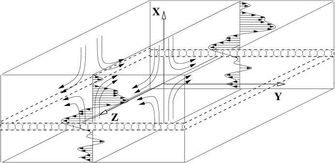
Attention is limited to the case where a series of parallel vortex sheets are formed at some instant, $t=t_{o},$ within a two dimensional potential flow, i.e., a strain rate field, given by $\mathbf{u}=[-kx,0,kz].$ See figure 1. The formation of each sheet occurs due to the appearance of a spatially varying flow component in the y-direction, given by

$$v(x,t=t_{o})=\sum_{i=1}^{N_{x}}\Delta v_{i}U(x-x_{i})$$ (61)

where $v=v_{y},$ $\Delta v_{i}$ is the incremental velocity at $x_{i},$ $U(x-x_{i})$ is the unit step function, and $N_{x}$ is the number of increments. There is no limit on the size of individual velocity increments; as shown immediately below, these determine the strength of each associated vortex sheet.

Figure 1: Continuous collection of Burger’s vortex sheets evolving under influence of an inviscid strain rate field, $v_{x}=-kx,v_{z}=kz.$ Vorticity is one-dimensional in the $z-\mathrm{direction}$ and is produced by the $y-\mathrm{velocity}$ component, $v_{y}(x,t).$

The vorticity equation assumes the linear 1-D form

$$\Omega_{t}-kx\Omega_{x}=k\Omega+\nu\Omega_{xx}$$ (62)

where $\Omega$ is directed along the $z-\mathrm{axis.}$ The initial condition associated with (61) is

$$\Omega(x,t=t_{o})=\sum_{i=1}^{N_{x}}\Delta v_{i}\delta(x-x_{i})$$ (63)

Due to the linearity of the governing equation (62), the last condition can be given a clear physical meaning: it corresponds to the superposition of $N_{x},$ infinitesimally thin vortex sheets, $\{\Omega_{i}\}_{1}^{N_{x}},$

$$\Omega(x,t=t_{o})=\sum_{i=1}^{N_{x}}\Omega_{i}(x_{i},t_{o})$$ (64)

where

$$\Omega_{i}(x_{i},t_{o})=\Delta v_{i}\delta(x-x_{i})$$ (65)

(and where units on $\delta(x-x_{i})=\frac{dU}{dx}$ are $\mathrm{length}^{-1}).$

The generic solution, describing the vorticity field produced by the $N_{x}$ sheets, is of the form:

$$\Omega(x,t)=\sum_{i=1}^{N_{x}}\Omega_{i}(x,t)$$ (66)

where the detailed form of $\Omega_{i}$ is given below.

6.2 Derivation of the single sheet Green’s function

We derive the single sheet Green’s function, $G^{(i)}(x,t|x_{i},t_{o}),$ by first normalizing (62) with the initial sheet strength, $\Delta v_{i},$ and then by noting that the resulting problem takes the form of that governing a forward time GF; see, e.g., [29]. Thus, we solve for $\Omega_{i}(x,t)/\Delta v_{i},$ and use

$$G^{(i)}(x,t|x_{o},t_{o})=\frac{\Omega_{i}(x,t)}{\Delta v_{i}}$$ (67)

where $x_{o}$ is the initial location of the infinitely thin vortex sheet. We take $t_{o}=0,$ temporarily drop superscripts and subscripts referring to sheet $i,$ and refer to the vorticity field produced as an individual Burger’s vortex sheet.

While Townsend’s 1951 paper [51] is cited by Saffman [52] as the source for a solution to a scalar transport problem occurring in a time-varying strain field of the type considered here, Townsend’s derivation, based on the method of characteristics (MOC), is apparently given elsewhere. Here, using a Fourier transform-MOC approach, representing a slightly generalized version of Gardiner’s solution for a one-dimensional OU process evolving in a steady drift field [8], we first derive a solution appropriate to time-varying strain fields of the form:

$$\mathbf{v}=-k(t)x\mathbf{e_{x}}+k(t)z\mathbf{e_{z}}$$ (68)

Fourier transforming (62) yields

$$\hat{\Omega}_{t}+k(t)\kappa\hat{\Omega}_{\kappa}+\nu\kappa^{2}\hat{\Omega}=0$$ (69)

Placing this in characteristic form then yields:

$$\frac{d\hat{\Omega}}{dt}=-\nu\kappa^{2}\hat{\Omega}\hskip 19.91684pt\mathrm{on}\hskip 19.91684pt\frac{d\kappa}{dt}=k(t)\kappa$$ (70)

Integrating along characteristics from $\kappa_{o}=\kappa(t_{o})$ to $\kappa=\kappa(t)$ yields

$$\kappa(t)=\kappa_{o}\exp[h(t)]$$ (71)

where

$$h(t)=\int_{t_{o}}^{t}k(t^{\prime})dt^{\prime}$$ (72)

Next, substituting (71) in (70) gives

$$\hat{\Omega}(\kappa,t)=\hat{\Omega}(k_{o},t_{o})\exp\big{[}-\nu k_{o}^{2}\int_{t_{o}}^{t}e^{2h(t^{\prime})}dt^{\prime}\big{]}$$ (73)

while setting the initial time $t_{o}=0$ and using the initial condition

$$\Omega(x,0)=\Delta v\delta(x-x_{o})$$ (74)

leads to

$$\hat{\Omega}(\kappa_{o},0)=\Delta ve^{i\kappa_{o}x_{o}}=\Delta v\exp[i\kappa e^{-h(t)}x_{o}]$$ (75)

Finally, letting

$$p(t)=e^{-2h(t)}\int_{0}^{t}e^{2h(t^{\prime})}dt^{\prime}$$ (76)

and taking the inverse transform of (73) leads to the final single-sheet Green’s function:

$$G(x,t|x_{o},t_{o}=0)=\frac{\Omega(x,t)}{\Delta v}=\frac{1}{\sqrt{4\pi\nu p(t)}}\exp{\big{[}\frac{-(x-x_{o}e^{-h(t)})^{2}}{4\nu p(t)}\big{]}}$$ (77)

The single sheet GF shows that peak response to the initial delta function travels to $x(t)=x_{o}e^{-h(t)}$ and spreads as $p(t).$ As a quick check, we note that in the case where $k(t)$ is constant, (77) assumes the appropriate form [53, 52].

In order to circumvent destabilizing vortex compression, it appears that for most times, $t,$ $k(t)$ must remain positive. Although short periods of vortex compression, sandwiched between long periods of stretching, can likely be stably sustained, we make no attempt to address this question. Rather, we limit attention, in the deterministic case, to $k(t)>0,$ and in the random case, $k(t)=k_{o}+k^{\prime}(t),$ to positive $k_{o},$ with $k_{o}>|k^{\prime}(t)|_{max},$ where $k_{o}$ and $k^{\prime}(t)$ are the non-random and random parts of $k(t).$

6.3 Vortex sheet evolution as an Ornstein-Uhlenbeck process

Focusing on the evolution of an individual BVS, say the $i^{th}$ sheet (having vorticity $\Omega_{i}(t))$ in a collection of $N_{x}$ sheets, again defining a normalized vorticity, $\tilde{\Omega}_{i}=\Omega_{i}/\Delta v_{i},$ and again noting the initial condition (65), we observe that equation (62) can also be interpreted as a Fokker-Planck equation governing the transition density,

$$p^{(i)}(x,t|x_{i},t_{o})=\frac{\Omega_{i}(x,t)}{\Delta v_{i}}$$ (78)

of an OU stochastic process $\chi^{(i)}(t),$ where $\chi^{(i)}$ evolves as:

$$d\chi^{(i)}(t)=-k(t)\chi^{(i)}(t)dt+\sqrt{2\nu}dw^{(i)}(t)$$ (79)

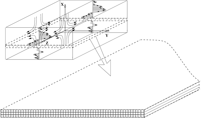
Importantly, this connection allows us to introduce a correspondence between the evolution of individual realizations of the stochastic process, $\chi^{(i)}(t),$ and evolution of individual elemental vortex sheets. In this picture, the instantaneous BVS, here the $i^{th}$ sheet, corresponds to a cloud of say $N$ elemental vortex sheets; see figure 2. Although we suppose for the moment that EVS’s are quasi-physical entities, analogous to say idealized, infinitely thin vortex sheets, we argue below that a physically reasonable embodiment of these can be defined; see section 6.4.2.

Figure 2: Decomposition of individual Burger’s vortex sheets into elemental vortex sheets.

Given a stochastic picture of BVS evolution, we can now easily write down physically meaningful expressions for the mean position of the vortex cloud $(=i^{th}$ Burger’s vortex sheet) $<\chi^{(i)}(t)>_{x},$ and it’s diffusive spread, i.e., its thickness, $<(\chi^{(i)}(t)-<\chi^{(i)}(t)>_{x})^{2}>_{x}:$

$$<\chi^{(i)}(t)>_{x}=\int_{-\infty}^{\infty}xp^{(i)}(x,t|x_{i},t_{o})dx$$ (80)

$$<(\chi^{(i)}(t)-<\chi^{(i)}(t)>_{x})^{2}>_{x}=\int_{-\infty}^{\infty}(x-<\chi^{(i)}(t)>_{x})^{2}p^{(i)}(x,t|x_{i},t_{o})dx$$ (81)

where expectations over the stochastic process, $\chi^{(i)}(t),$ are written in the notationally convenient form, $<\cdot>_{x}.$

When the strain rate $k(t)$ is random (see sections 6.6 and 6.7), equations (62), (65), (79)-(81) apply to any realization of $k(t).$ Thus, following, e.g., [55, 56, 57], the average sheet position and spread over random $k$ will be computed as:

$$\big{<}<\chi^{(i)}(t)>_{x}\big{>}=\big{<}\int_{-\infty}^{\infty}xp^{(i)}(x,t|x_{i},t_{o})dx\big{>}$$ (82)

and

$$\big{<}<(\chi^{(i)}(t)-<\chi^{(i)}(t)>_{x})^{2}>_{x}\big{>}=\big{<}\int_{-\infty}^{\infty}(x-<\chi^{(i)}(t)>_{x})^{2}p^{(i)}(x,t|x_{i},t_{o})dx\big{>}$$ (83)

where expectations taken with respect to $k$ will be denoted as $<\cdot>.$

6.4 Elemental vortex sheets

In order to develop a physically and mathematically consistent picture of EVS’s, we limit attention to incompressible flows and consider vorticity transport on length and time scales that are small relative to those associated with BVS dynamics.

In order to identify an appropriate time scale, we first appeal to the Biot-Savart law:

$$\mathbf{v_{s}}(\mathbf{x},t)=-\frac{1}{4\pi}\int\frac{\mathbf{r}\mathbf{\times}\boldsymbol{\omega}(\mathbf{y},t)}{r^{3}}d\mathbf{y}$$ (84)

where $\mathbf{r}=\mathbf{x}-\mathbf{y}.$ This kinematic result, which gives the instantaneous solenoidal (incompressible) velocity field, $\mathbf{v_{s}},$ in terms of an integral over the vorticity field, $\boldsymbol{\omega},$ indicates that the local magnitude and direction of the former instantaneously senses and responds to the integrated effects of the latter. In reality, sensing and response are acoustically mediated.

Thus, we surmise that in order to expose sub-sheet dynamics, we should focus on processes taking place on acoustic time scales. This choice, in fact, proves advantageous since the acoustic scale lies well separated from both the much longer BVS time scale, $k^{-1},$ and the much shorter molecular collision scale, $\tau_{c},$ given below; as will be shown, substantial insight into sub-sheet rotational dynamics emerges on this intermediate scale.

For the EVS length scale, we focus on lengths that are large relative to molecular scales, $d_{o},$ and small relative to the characteristic BVS thickness, $\delta_{i}(t),$ where, depending on whether the strain rate field is deterministic or not, $\delta_{i}(t)$ is given, respectively, by (81) or (83).

Thus, as a means of gaining a conceptual foothold, it proves useful to focus on the acoustic time scale, near-molecular length scale rotational dynamics and evolution of in-sheet clumps, fluid particles comprised of a fixed number of say $N_{cl}$ molecules. Limiting attention to liquids, and given a characteristic (effective) molecular diameter $d_{o},$ the characteristic clump size is $\delta_{cl}\approx N_{cl}^{1/3}d_{o}.$

For a short period, $\tau_{cl},$ any given clump remains nominally intact and experiences an incremental rotation, the magnitude of which corresponds to the average rotation of all constituent molecules. Since clump dispersion occurs due to thermal motion of constituent molecules, $\tau_{cl}\approx\delta_{cl}/v_{T},$ where $v_{T}=\sqrt{3kT/m},$ the thermal speed, is on the order of the sound speed, $a_{o}.$

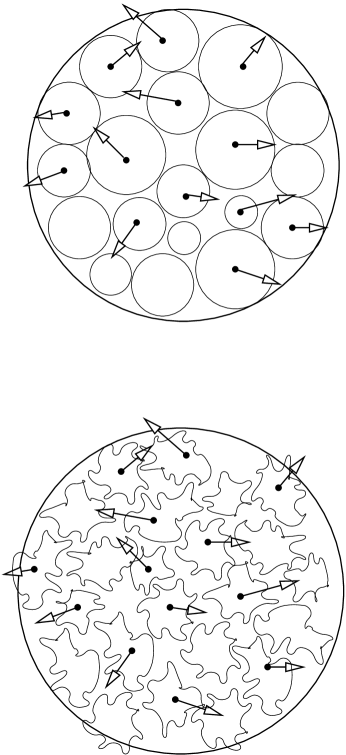
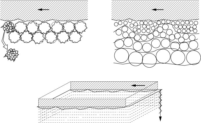
Since the ratio of $\tau_{cl}$ to the collision time scale, $\tau_{c}=O(d_{o}/v_{T}),$ is $O(N_{cl}^{1/3}),$ choosing $N_{cl}$ to be on the order of say, $10^{3},$ gives $\tau_{cl}/\tau_{c}=O(10).$ Hence, as depicted in figure 3, we envision that an initially smooth collection of clumps becomes ’bumpy’, i.e., thermally roughened, over a time interval of $O(\tau_{cl});$ likewise, as noted in the caption, individual clumps remain largely intact.

Figure 3: Over a time interval on the order of $\tau_{cl},$ an initially smooth collection of neighboring clumps begins to thermally disperse. Since the clump is large relative to individual constituent molecules, dispersion on this time scale takes place predominantly via thermal roughening and inter-penetration of surface molecules (where the latter are depicted as surface bumps). Holes within, and penetrating jets into, clumps form as well, but the fraction of molecules having sufficient energy to form these over $\tau_{cl}$ is small; thus, these are not depicted.

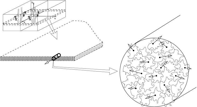
Indeed, the $\tau_{cl}-\mathrm{scale}$ inter-clump transfer of rotational momentum can be viewed as a consequence of the cog-like action of clump-surface molecules interacting with one another. Figure 4 provides a schematic representation of vortex sheet vorticity on the large BVS scale, the smaller elemental vortex scale, and on the clump-scale.

Figure 4: On acoustic time scales and on the elemental vortex length scale, vorticity corresponds to the instantaneous average rotation of $N_{cl}$ molecules comprising a fluid clump. On these short time and length scales, and under subsonic conditions, the vorticity field is three-dimensional, disordered, and strongly diffusive.

Qualitative insight into clump-scale dynamics can be gained by assuming that a continuum description applies on scales of order $\delta_{cl}$ and $\tau_{cl}.$ Recognizing that clump-scale gradients in BVS-scale velocities and vorticities are small and nondimensionalizing the full vorticity transport equation, we obtain:

$$\boldsymbol{\tilde{\omega}}_{\tilde{t}}-\mathrm{Re}^{-1}\tilde{\nabla}^{2}\boldsymbol{\tilde{\omega}}=-\mathrm{Ma}\boldsymbol{\hat{u}}\cdot\boldsymbol{\tilde{\nabla}}\cdot\boldsymbol{\tilde{\omega}}$$ (85)

where $\mathrm{Re}^{-1}=\nu/(a_{o}\delta_{cl})$ is a clump-scale Reynolds number, $\mathrm{Ma}=u_{s}/a_{o}$ is a BVS-scale mach number, $u_{s}=O(kx_{s})$ is the BVS velocity scale, $x_{s}$ is the BVS-scale sheet position, and where we have dropped a $O(\delta_{cl}/x_{s})$ term describing stretching of BVS-scale vorticity by the clump-scale velocity field.

Note first that for liquids like water, and for clumps having $O(10^{3})$ molecules, $Re=O(1).$ Under these circumstances, and under conditions where the BVS-scale mach number is small, (85) shows that, relative to diffusion, clump-scale stretching (again, dropped from (85)) and advection of vorticity are likewise small. This is consistent with a detailed analysis of organization of clump-scale vorticity by in-sheet hydrodynamic modes below (section 6.4.1); there, it is shown that diffusional smoothing via shear and entropy modes constitute two of three hydrodynamic organizing mechanisms.

Thus, from (85), the following picture of clump-scale vorticity transport emerges:

1. in low speed incompressible flows $(Ma<<1),$ transport is three dimensional and diffusive,

2. advection, important on BVS length and time scales, only emerges on the clump-scale when liquid bulk velocities are high, on the order of the sound speed, and

3. stretching remains weak to the point of nonexistence.

6.4.1 Organization of clump-scale vorticity: hydrodynamic modes

Given that vorticity transport on BVS scales is highly organized and one dimensional, evolving on these scales under the combined action of advection, stretching, and diffusion, while sub-sheet (clump-scale) transport is highly disorganized, three dimensional, and diffusive, it becomes apparent that some mechanism, acting over time and length scales long relative to $\delta_{cl}$ and $\tau_{cl},$ organizes disordered clump-scale vorticity.

We assume that the organizing mechanism is associated with weak hydrodynamic modes superposed on the bulk, BVS-scale velocity field. In order to expose the role of these modes on sub-sheet organization, we focus on a simpler analog problem, organization in unstrained vortex sheets $(k=0).$

The analysis adapts Mountain’s [58] well known approach for analyzing the small wave number, low frequency response of simple liquids to excitation via scattered inelastic light and neutron beams [58, 59, 9]. In the scattering problem, a probe beam interrogates a (nominally) static liquid, with the scattered beam then detected and analyzed.

Here, we assume that the source of excited hydrodynamic modes within the vortex sheet derives from the feature generating sheet-scale vorticity, e.g., a solid or fluid body moving relative to the initially static liquid. In contrast to the beam scattering problem [58, 59, 9], we must include the space- and time-dependent background velocity field, $\mathbf{\bar{u}}=u(y,t)\mathbf{\hat{e}_{x}},$ produced by the vortex sheet.

Model assumptions are as follows:

1. Due to homogeneity of downstream (x-direction) and cross-stream (z-direction) boundary conditions at the moving, vorticity-generating boundary or fluid interface, we assume that hydrodynamic fluctuations vary only in the cross-sheet (y-) direction.

2. For the same reason, we assume that only one hydrodynamic shear momentum current, i.e., mass weighted vorticity component, $\mu_{z}(y,t)=\rho\boldsymbol{\nabla}\mathbf{\times}\mathbf{v}\cdot\mathbf{\hat{e}_{z}},$ appears and that it is directed in the cross-stream (z-) direction.

3. Consistent with the discussion above, we assume that hydrodynamic fluctuations take place on time and length scales that are short relative to those of the vortex sheet, and long relative to $d_{o}$ and $\tau_{cl}.$

Thus, express the field variables, $s,$ $p,$ $w,$ and $\mu_{z},$ as the superposition of a slowly varying, sheet-scale component, $\bar{f}(\bar{y},\bar{t}),$ and a weak fluctuating sub-sheet component, $f^{\prime}(y,t):$

$$f(y,\bar{y},t,\bar{t})=\bar{f}(\bar{y},\bar{t})+f^{\prime}(y,t)$$ (86)

where $s,$ $p,$ and $w=\rho\boldsymbol{\nabla}\cdot\mathbf{v}=\rho\boldsymbol{\nabla}\cdot\mathbf{v^{\prime}}$ are, respectively, the entropy, pressure, and dilatational momentum currents. In order to expose sub-sheet-scale processes, sheet-scale time and position coordinates, $\bar{y}$ and $\bar{t},$ are magnified using

$$\bar{y}=\epsilon y$$

$$\bar{t}=\epsilon_{1}t$$

where $y$ and $t$ are hydrodynamic-scale coordinates and where

$$\epsilon=d_{c}/\delta_{i}$$

$$\epsilon_{1}=\tau_{cl}/(d_{c}/a_{o})$$

Thus, on the sub-sheet, hydrodynamic scale, time and space derivatives of $f$ are given by:

$$\frac{\partial f}{\partial y}=\epsilon\frac{\partial\bar{f}}{\partial\bar{y}}+\frac{\partial f^{\prime}}{\partial y}$$

$$\frac{\partial f}{\partial t}=\epsilon_{1}\frac{\partial\bar{f}}{\partial\bar{t}}+\frac{\partial f^{\prime}}{\partial t}$$ (87)

In other words, on the sub-sheet scale, variations in sheet-scale fields are small.

Extending the approach in [59] to the problem of hydrodynamic fluctuations within a planar vortex sheet, we derive the following system of equations governing $s^{\prime},$ $p^{\prime},$ $w^{\prime},$ and $\mu_{z}^{\prime}:$

$$\begin{array}[]{rcl}\left[\frac{\partial}{\partial t}-(k-1)\alpha_{T}\nabla^{2}\right]p^{\prime}(y,t)+a_{o}^{2}w^{\prime}(y,t)-\bar{\rho}\beta^{-1}(k-1)\alpha_{T}\nabla^{2}s^{\prime}(y,t)=&F_{1}&=O(\epsilon,\epsilon_{1})\\ \left[\frac{\partial}{\partial t}-(\frac{4}{3}\nu+\nu_{B})\nabla^{2}\right]w^{\prime}(y,t)+\nabla^{2}p^{\prime}(y,t)=&F_{2}&=O(\epsilon,\epsilon_{1})\\ \left[\frac{\partial}{\partial t}-\alpha_{T}\nabla^{2}\right]s^{\prime}(y,t)-\beta\bar{\rho}^{-1}\alpha_{T}\nabla^{2}p^{\prime}(y,t)=&F_{3}&=O(\epsilon,\epsilon_{1})\\ \left[\frac{\partial}{\partial t}-\nu\nabla^{2}\right]\mu_{z}^{\prime}(y,t)=&F_{4}&=O(\epsilon,\epsilon_{1})\end{array}$$ (88)

where $k=C_{p}/C_{v}$ is the ratio of specific heats, $\alpha_{T}$ is the thermal diffusivity, $a_{o}$ is the adiabatic sound speed, $\beta$ is the coefficient of thermal expansion, and $\nu=\mu/\bar{\rho}$ and $\nu_{B}=\mu_{B}/\bar{\rho},$ where $\mu$ and $\mu_{B}$ are the shear and bulk viscosity coefficients, respectively.

Prior to listing the $O(\epsilon,\epsilon_{1})$ terms on the right above, we define

$$F_{o}=\frac{1}{\bar{\rho}\bar{T}}\left[-(\rho^{\prime}\bar{T}+T^{\prime}\bar{\rho})\frac{\partial\bar{s}}{\partial t}+\boldsymbol{\Delta^{\prime}}\cdot\boldsymbol{\pi}+\boldsymbol{\Delta}\cdot\boldsymbol{\pi^{\prime}}\right]$$ (89)

where $\Delta_{ij}=(v_{i,j}+v_{j,i})/2$ is the rate of deformation tensor and $\pi_{ij}=2\eta_{1}\Delta_{ij}+\eta_{2}\Delta_{ij}\delta{ij}$ is the stress tensor, and $\eta_{1}$ and $\eta_{2}$ are the shear viscosity and dilatational viscosity, respectively (with $\eta_{1}=\mu$ and $2\eta_{1}+\eta_{2}=\frac{4}{3}\mu+\mu_{B}).$ Primes on $\Delta_{ij}$ and $\pi_{ij}$ denote tensors in the hydrodynamic velocity component; here, only derivatives in the cross-sheet $(y-)$ direction appear. It is seen that products of primed and unprimed versions of $\boldsymbol{\Delta}$ and $\boldsymbol{\pi}$ represent viscous dissipation due to weak $O(\epsilon,\epsilon_{1})$ interaction between hydrodynamic-scale and sheet-scale velocity fields.

Given $F_{o},$ the $O(\epsilon,\epsilon_{1})$ terms above can be expressed as: $F_{1}=(k-1)\bar{\rho}\beta^{-1}F_{o},$ $F_{2}=-\mathbf{\bar{v}}_{t}\cdot\rho^{\prime}-\bar{\rho}v_{j,i^{\prime}}\bar{v}_{i,j},$ $F_{3}=F_{o},$ and $F_{4}=-\bar{\rho}^{-1}\boldsymbol{\nabla}\mathbf{\times}(\rho^{\prime}\mathbf{\bar{v}}_{t})-\boldsymbol{\nabla}\mathbf{\times}[\mathbf{v^{\prime}}\cdot\boldsymbol{\nabla}\mathbf{\bar{v}}].$

Importantly, the $O(1)$ left hand side of (88) is, with the exception of the appearance of one rather than two shear momentum currents, identical to that describing the hydrodynamic response of a nominally static liquid to beam scattering. Thus, focusing on the leading order problem, we can immediately apply the results of the scattering problem to sub-sheet organization in unstrained vortex sheets. Taking the Laplace-Fourier transform of the above system

$$\hat{f^{\prime}}_{k}=\int_{0}^{\infty}\int_{-\infty}^{\infty}e^{i\mathbf{k}\cdot\mathbf{x}}e^{-st}f^{\prime}(\mathbf{x},t)d\mathbf{x}dt$$

with $\mathbf{x}=y\mathbf{\hat{e}_{y}},$ and enforcing the solvability condition leads to

$$\left|\begin{array}[]{cccc}[s+(k-1)\alpha_{T}k^{2}]&a_{o}^{2}&\bar{\rho}\beta^{-1}(k-1)\alpha_{T}k^{2}&0\\ -k^{2}&[s+\nu_{l}k^{2}]&0&0\\ \bar{\rho}^{-1}\beta k^{2}&0&[s+\alpha_{T}k^{2}]&0\\ 0&0&0&[s+\nu k^{2}]\end{array}\right|=0$$ (90)

From the original system (or (90)), it is clear that the cross-sheet shear momentum current is uncoupled from the other three modes; from (90), the associated dispersion relation

$$s_{4}=-\nu k^{2}$$ (91)

shows that this mode is purely diffusive. The remaining modes follow from (90) and are given by [58, 59]:

$$s_{1} =-\alpha_{T}k^{2}$$ (92)

$$s_{2,3} =\pm ia_{o}k-A_{o}k^{2}$$ (93)

where $A_{o}=[\nu_{l}+(k-1)\alpha_{T}]/2,$ with $\nu_{l}=\frac{4}{3}\nu+\nu_{B}.$

Thus, from (92) and (93), we surmise that, beyond cross-sheet diffusion of clump-scale vorticity, two additional sub-sheet organizing mechanisms act (respectively): thermal smoothing via a purely diffusive cross-sheet entropy mode, and acoustic smoothing via weakly damped, oppositely-directed, cross-sheet acoustic modes (with the rate of damping determined by $A_{o}).$

Physically, in the cross-sheet direction, acoustic dilatational waves tend to push out-of-plane vorticity fluctuations into a planarized configuration; likewise, within the in-sheet plane, wave reflection between neighboring vorticity fluctuations tend to align the fluctuations in the $z-\mathrm{direction}.$ Superposed on these acoustic mechanisms, diffusional smoothing of clump-scale vorticity as well diffusion of friction-generated thermal energy provide additional, strongly organizing effects. The mechanisms are depicted in figure 5; see the caption for further discussion.

Figure 5: Organization of disordered clump-scale vorticity is mediated by three hydrodynamic modes: a diffusive, cross-sheet entropy (thermal) mode (upper left), a diffusive, cross-sheet shear (vorticity) mode (upper right), and a pair of counter-propagating, weakly damped, cross-sheet acoustic modes (bottom). We depict the thermal mode in terms of the thermal degradation (dispersion) of in-sheet clumps. The vorticity mode can likewise be viewed as the hydrodynamic-time-scale clump-to-clump transfer of rotational inertia. On these time scales, clumps experience significant dispersion so that rotational transport takes place by both the cog-like interaction of adjacent ’thermal bumps’, and gross intermixing of neighboring clumps.

6.4.2 Elemental vortex sheets defined

Having developed a physical picture of sub-BVS vorticity, we can identify a reasonable physical embodiment of the sub-BVS scale stochastic processes defined by equation (79): elemental vortex sheets are defined as planar vorticity layers of thickness $O(\delta_{cl}),$ which evolve stochastically within any given BVS, on the long BVS time-scale.

Two features suggest that EVS’s can be taken as real, rather than quasi-physical, entities. First, since hydrodynamic acoustic, shear, and entropy modes organize, on long BVS length and time scales, disordered small- (clump-) scale vorticity, it is clear that these long-acting modes are likewise capable of organizing $O(\delta_{c})$ layers of vorticity. Thus, on BVS time scales, it is physically reasonable to view, at any instant, a Burger’s vortex sheet, or any vortex sheet, as being composed of $O(\delta_{i}/\delta_{cl})$ elemental vortex sheets. Additionally, it is likewise reasonable to expect that due to long-time-scale organization of short-time-scale vorticity, $O(\delta_{cl})$ layers of vorticity evolve stochastically, en mass, over long BVS time increments, $\Delta t.$

6.5 Vortex sheet evolution in non-random strain rate fields

Prior to discussing vortex sheets in random strain rate fields, we briefly consider physically interesting aspects of the solution which apply to non-random strain fields. Thus, using (77) in (66), one can write down the vorticity field produced by $N_{x}$ initially discrete Burger’s vortex sheets:

$$\Omega(x,t)=\sum_{i=1}^{N_{x}}\frac{\Delta v_{i}}{\sqrt{4\pi\nu p(t)}}\exp\big{[}\frac{-(x-x_{i}e^{-h(t)})^{2}}{4\pi\nu p(t)}\big{]},$$ (94)

where again, $\Delta v_{i}$ is the incremental change in the streamwise velocity at $x_{i}.$

Several observations follow from this solution. First, from (80) and (81), the mean position and diffusive spread of the $i^{th}$ sheet, viewed as the stochastic evolution of a cloud of elemental vortex sheets, are given respectively by:

$$<\chi_{i}(t)>_{x}=x_{i}\exp\big{(}{-h(t)}\big{)}$$ (95)

and

$$<(\chi_{i}(t)-<\chi_{i}(t)>_{x})^{2}>_{x}=2\nu p(t)$$ (96)

where $h(t)$ and $p(t)$ are given by (72) and (76). Thus, in non-random strain rate fields (and due to the linearity of the problem), each sheet (in the collection of $N_{x}$ sheets) migrates toward $x=0,$ each diffusively spreading at a spatially uniform rate; at large times, all $N_{x}$ sheets coalesce at $x=0,$ with the thickness of the collection, $\sqrt{2\nu p(t)},$ identical to that of a single sheet. In the case where $k(t)$ is constant, the above mean and variance simplify to those for the equivalent OU process considered in [8]. Likewise, identifying $\sqrt{<(\chi_{i}(t)-<\chi_{i}(t)>_{x})^{2}>_{x}}$ as the thickness of sheet $i,$ we obtain the constant strain rate expressions for sheet position and thickness given, e.g., in [53, 52].

Second, and considering the long-time strength of the composite sheet in the case where $k$ is either (a positive) constant or approaches a long-time limit, $k\rightarrow k_{\infty},$ $h(t)\rightarrow\infty$ and $p(t)\rightarrow 1/(2k_{\infty}),$ and the strength of the coalesced collection of $N_{x}$ sheets, from (94), is the sum of the initial strengths:

$$v_{\infty}=\sum_{i=1}^{N_{x}}\Delta v_{i}$$ (97)

Thus, for example, when the strength of one of the initial sheets dominates all others, corresponding to a locally large change in the initial stream-wise velocity profile, (97) shows that the final sheet strength is largely determined by the strength of this sheet. In contrast, in situations where the initial streamwise velocity profile takes on positive and negative magnitudes, and more specifically, is characterized by a limited number of Fourier modes, (97) shows that due to vorticity cancellation the final strength is small.

6.6 Single and continuous sets of Burger’s vortex sheets in random strain rate fields

Focusing first on the dynamics of a single vortex sheet $(N_{x}=1$ in (94)), we note that since equations (94), (95), and (96) apply to individual realizations of $k(t),$ then the corresponding ensemble averaged instantaneous vorticity, sheet position, and sheet thickness, taken over $k,$ can be expressed respectively as:

$$\big{<}\Omega(x,t)\big{>}=\big{<}\frac{\Delta v}{\sqrt{4\pi\nu p(t)}}\exp\big{[}\frac{-(x-x_{o}e^{-h(t)})^{2}}{4\pi\nu p(t)}\big{]}\big{>}$$ (98)

$$\big{<}<\chi(t)>_{x}\big{>}=x_{o}\big{<}\exp\big{(}{-h(t)}\big{)}\big{>}$$ (99)

and

$$\big{<}<(\chi(t)-<\chi(t)>_{x})^{2}>_{x}\big{>}=2\nu\big{<}p(t)\big{>}$$ (100)

where $h(t)$ and $p(t)$ are again given by (72) and (76), and $\Delta v$ is the incremental (step-function) change in the streamwise velocity at $x_{o}.$

Explicit formulas for these quantities can be obtained when the strain rate field is statistically stationary, has positive mean, and a gaussian random component:

$$k(t)=k_{o}+k^{\prime}(t)$$ (101)

where, for stability, we assume a condition like $k_{o}^{2}>\alpha\big{<}(k^{\prime})^{2}\big{>},$ where $\alpha$ is an undetermined positive number. Under these conditions [60]:

$$\Big{<}\exp\big{[}-\int_{0}^{t}k^{\prime}(s)ds\big{]}\Big{>}=\exp\big{[}\frac{1}{2}\int_{0}^{t}\int_{0}^{t}\big{<}k^{\prime}(s)k^{\prime}(s^{\prime})\big{>}dsds^{\prime}\big{]}$$ (102)

Inserting the correlation function, $R,$ and using the property

$$R(|\tau|)=\big{<}k^{\prime}(t^{\prime}+\tau)k^{\prime}(t^{\prime})\big{>}$$ (103)

appropriate to stationary processes, allows restatement of (102) in the form:

$$\Big{<}\exp\big{[}-\int_{0}^{t}k^{\prime}(s)ds\big{]}\Big{>}=\exp\big{[}\frac{1}{2}\int_{0}^{t}\int_{0}^{t}R(|s-s^{\prime}|)dsds^{\prime}\big{]}$$ (104)

In turn, the identity [57]

$$\frac{1}{2}\int_{0}^{t}\int_{0}^{t}R(|s-s^{\prime}|)dsds^{\prime}=\int_{0}^{t}(t-s)R(|s|)ds$$ (105)

is useful when evaluating the right side of (104).

Thus, inserting (104) and (105) in (99) yields the following formula for the (single) sheet’s ensemble average position, applicable to random strain fields of the form in (101):

$$\big{<}<\chi(t)>_{x}\big{>}=x_{o}e^{-k_{o}t}\exp\big{[}\int_{0}^{t}(t-s)R(|s|)ds\big{]}$$ (106)

In order to obtain the corresponding single sheet spread, we use (76) to write

$$\big{<}p(t)\big{>}=e^{-2k_{o}t}\big{<}\exp{\big{[}-2\int_{0}^{t}k^{\prime}(t^{\prime})dt^{\prime}\big{]}}\cdot\int_{0}^{t}\Big{(}e^{2k_{o}t^{\prime}}\exp{\big{[}2\int_{0}^{t^{\prime}}k^{\prime}(s^{\prime})ds^{\prime}\big{]}}\Big{)}dt^{\prime}\big{>}$$ (107)

and assume that the two terms separated by the center dot represent independent random variables:

$$\big{<}p(t)\big{>}=e^{-2k_{o}t}\big{<}\exp{\big{[}-2\int_{0}^{t}k^{\prime}(t^{\prime})dt^{\prime}\big{]}}\big{>}\cdot\big{<}\int_{0}^{t}\Big{(}e^{2k_{o}t^{\prime}}\exp{\big{[}2\int_{0}^{t^{\prime}}k^{\prime}(s^{\prime})ds^{\prime}\big{]}}\Big{)}dt^{\prime}\big{>}$$ (108)

or

$$\big{<}p(t)\big{>}=e^{-2k_{o}t}\big{<}\exp{\big{[}-2\int_{0}^{t}k^{\prime}(t^{\prime})dt^{\prime}\big{]}}\big{>}\cdot\int_{0}^{t}\Big{(}e^{2k_{o}t^{\prime}}\big{<}\exp{\big{[}2\int_{0}^{t^{\prime}}k^{\prime}(s^{\prime})ds^{\prime}\big{]}}\big{>}\Big{)}dt^{\prime}$$ (109)

Using (104) and (105) to evaluate the expectations in (109) and inserting the results in (100) then yields:

$$\big{<}<(\chi(t)-<\chi(t)>_{x})^{2}>_{x}\big{>}=2\nu e^{-2k_{o}t}\exp\big{[}4\int_{0}^{t}(t-s)R(|s|)ds\big{]}\cdot\int_{0}^{t}\Big{(}e^{2k_{o}t^{\prime}}\exp\big{[}4\int_{0}^{t^{\prime}}(t^{\prime}-s^{\prime})R(|s^{\prime}|)ds^{\prime}\big{]}\Big{)}dt^{\prime}$$ (110)

Considering, for illustration, the case where the random strain field is delta correlated in time

$$\big{<}k^{\prime}(t^{\prime}+\tau)k^{\prime}(t^{\prime})\big{>}=\tilde{k}\delta(\tau)$$ (111)

where $\tilde{k}$ is a positive constant (determined, e.g., by experiment), one finds that sheet spread no longer approaches a fixed long-time limit (as in the case of deterministic strain rate), but rather exhibits exponential, i.e., superdiffusive [61] growth:

$$\big{<}<(\chi(t)-<\chi(t)>_{x})^{2}>_{x}\big{>}=\frac{\nu}{k_{o}+2\tilde{k}}\exp\Big{(}8\tilde{k}t\big{[}1-\exp\big{(}-(2k_{o}+4\tilde{k})t\big{)}\big{]}\Big{)}$$ (112)

In the limit of weak random strain, specifically $\tilde{k}t<<1$ and $k_{o}>>\tilde{k},$ (112) simplifies to the constant strain (non-random) solution [8]:

$$\big{<}<(\chi(t)-<\chi(t)>_{x})^{2}>_{x}\big{>}=\frac{\nu}{k_{o}}\big{[}1-\exp\big{(}-2k_{o}t\big{)}\big{]}$$ (113)

[See section 6.7.1 below for a brief description of the conditions necessary for introducing an assumption of delta correlated strain rates.]

6.6.1 Continuous collections of Burger’s vortex sheets: Feynman-Kac solution

Turning to the case of multiple Burger’s vortex sheets, we consider the general case where the initial streamwise velocity component exhibits a continuous variation in the $x-$ direction,

$$v(x,0)=v_{o}(x)$$ (114)

Here, a representative solution for the mean continuous vorticity, $\big{<}\omega(x,t)\big{>},$ can be obtained using the Feynman-Kac solution [20] of the backward-time version of the vorticity equation (62):

$$\big{<}\Omega(x,t)\big{>}=\big{<}E_{\chi(t)=x,t}\big{[}\Omega(\chi(0),0)\big{]}\big{>}\cdot\big{<}e^{h(t)}\big{>}$$ (115)

where $E_{\chi(t),t}$ denotes the expectation associated with the stochastic process $\chi$ sampling the initial condition, $\Omega(x,0).$

As a quick check of this formula, we note that when $k(t)=k_{o}$ is non-random and constant and $v_{o}=c_{o}x,$ i.e., the initial streamwise velocity is of Couette form, the solution in (115) yields

$$\Omega(x,t)=c_{o}e^{k_{o}t}$$ (116)

This solution in turn satisfies the vorticity transport equation, (62), along with the initial condition, $\Omega(x,0)=c_{o}.$ Equation (116) holds under conditions where the time scale for setting up the Couette profile, say $\tau,$ is short relative to the strain field time scale, $\tau_{s}=k_{o}^{-1}.$ On the longer scale, diffusion of vorticity saturates out quickly and the appropriate initial condition, to order $k_{o}^{-1}/\tau,$ is $\Omega(x,0)=c_{o}.$ Under these conditions, the initial vorticity, $c_{o},$ is exponentially amplified by stretching.

As shown immediately below, in the case where $k(t)$ is random and $v_{o}$ again equals $c_{o}x,$ the Feynman-Kac solution in (115) coincides with the leading order low-viscosity (high Reynolds number) forward-time solution of (62). The paradox of the viscous solution coinciding with the inviscid solution is resolved by requiring (in analogy with the deterministic strain case immediately above), that for every realization of $k(t),$ the initial (linear) streamwise velocity profile forms on time scales much shorter than say, $|k^{-1}(t)|_{max};$ for each realization, diffusive effects again saturate out over the short time scale. We now briefly consider the latter, low viscosity problem.

6.7 Single-sheet and collective behavior under inviscid conditions

In the case of single sheets, significant questions include the effects of random strain on time-varying mean (ensemble averaged) sheet strength, position, and spread, while in the case of sheet collections, the key question centers on evolution of the ensemble average (position and time-dependent) vorticity. Attention is again focused on the case where $k(t)$ is given by (101) with $k^{\prime}(t)$ again a stationary zero-mean gaussian process.

Considering first single sheets, the position of the sheet under the action of an individual realization of $k(t),$

$$\chi(t)=e^{-h(t)}\chi(0)$$ (117)

follows either from the SDE governing the motion of elemental vortex sheets, (79), with the stochastic term suppressed, or by noting from the MOC solution for $\Omega(x,t)$ (using the inviscid form of (62)) that any given sheet evolves along characteristics given by (70). In the case of elemental sheets, since no diffusion takes place, all EVS’s within the Burger’s sheet evolve identically under the action of any given realization of $k(t).$ In the following, we express the sheet’s initial position as $\chi(0)=x_{o}.$

Given $\chi(t),$ the ensemble average sheet position over the random strain rate field can be calculated using (104) and (105):

$$\big{<}\chi(t)\big{>}=x_{o}e^{-k_{o}t}\big{<}\exp\big{[}-\int_{0}^{t}k^{\prime}(s)ds\big{]}\big{>}=x_{o}e^{-k_{o}t}\exp\left[\int_{0}^{t}(t-s)R(|s|)ds\right]$$ (118)

Since $(t-s)R(|s|)$ is positive for $s<t,$ then it is seen that any stationary random strain rate field inhibits sheet migration toward the origin, $x=0.$

Given $\big{<}\chi(t)\big{>},$ the sheet spread (or squared thickness), $\sigma_{\chi}^{2},$ can again be calculated:

$$\sigma_{\chi}^{2}=\Big{<}(\chi(t)-\big{<}\chi\big{>})^{2}\Big{>}=x_{o}^{2}e^{-2k_{o}t}\big{[}\big{<}\exp-2\int_{0}^{t}k^{\prime}(t^{\prime})dt^{\prime}\big{>}-\big{<}\exp-\int_{0}^{t}k^{\prime}(t^{\prime})dt^{\prime}\big{>}^{2}\big{]}$$ (119)

or

$$\sigma_{\chi}^{2}=x_{o}^{2}e^{-2k_{o}t}\big{[}\exp[4\int_{0}^{t}R(|s|)(t-s)ds]-\exp[2\int_{0}^{t}R(|s|)(t-s)ds]\big{]}$$ (120)

6.7.1 Inviscid vortex evolution in a rapidly decorrellating random strain rate field

This example briefly considers the spread of a single Burger’s vortex sheet under conditions where the correlation time, $\tau_{c}=\int_{0}^{\infty}\left<k^{\prime}(t)k^{\prime}(0)\right>dt/\mathrm{var}(k^{\prime}),$ of the random strain field, $k^{\prime}(t),$ is short relative to the time scale, $\tau_{b},$ associated with the vorticity-inducing flow, $v(x,t).$ Thus, define a normalized correlation function $\eta(\tau)=\left<k^{\prime}(\tau)k^{\prime}(0)\right>/c_{1}^{2},$ where $c_{1}^{2}$ is a normalization factor obtained from $\int_{-\infty}^{\infty}\eta(\tau)d\tau=1.$ In addition, let $\epsilon=\tau_{c}/\tau_{b}<<1,$ and renormalize the correlation function to the longer BVS time scale: $\eta_{\epsilon}(\tilde{\tau})=\epsilon^{-1}\eta(\epsilon^{-1}\tau),$ where $\tilde{\tau}=\tau/\epsilon.$ Since $\eta_{\epsilon}(\tilde{\tau})\rightarrow\delta(\tilde{\tau})$ as $\epsilon\rightarrow 0$ (and $\tilde{\tau}=O(\tau_{b})),$ then it is clear that the assumption of delta correlated statistics on the BVS time scale becomes increasingly valid as the ratio of the $\tau_{c}/\tau_{b}$ becomes increasingly small.

Thus, let $k^{\prime}(t)$ be delta correlated. In this case, (118) yields:

$$\big{<}\chi(t)\big{>}=x_{o}e^{(-k_{o}+\tilde{k})t}$$ (121)

Although this suggests that for large enough random strain, $\tilde{k}>k_{o},$ the mean position of the BVS can track away from the origin, $x=0,$ this cannot be confirmed without detailed consideration of sheet stability under random strain rates.

Under the same assumption, a variety of interesting long-time behaviors emerge, depending on the size of $\tilde{k}$ relative to $k_{o}:$

$$\sigma_{\chi}^{2}=x_{o}^{2}e^{-2k_{o}t}\big{[}e^{4\tilde{k}t}-e^{2\tilde{k}t}\big{]}$$ (122)

In particular:

1. when $\tilde{k}<k_{o}/2,$ corresponding to mean strain dominating the random component, sheet thickness goes to $0$ (i.e., $\sigma_{\chi}^{2}\rightarrow 0)$ as $t\rightarrow\infty;$

2. when $\tilde{k}>k_{o}/2,$ sheet thickness grows without bound $(\sigma_{\chi}^{2}\rightarrow\infty)$ as $t\rightarrow\infty;$

3. in the special case where $\tilde{k}=k_{o}/2,$ a fixed, non-zero thickness can be achieved, $\sigma_{\chi}\rightarrow x_{o}$ as $t\rightarrow\infty,$ indicating, both here and in the other cases, that the random strain functions as an effective agent for diffusion.

In each case, the increase in sheet spread amplitude with initial position, $x_{o}^{2},$ reflects the increase in random velocity amplitude, $v^{\prime}(x,t)=k^{\prime}(t)x^{\prime},$ with $x.$ Finally, and once again, cases ii) and iii) are subject to the proviso concerning sheet stability in increasingly random strain fields.

6.7.2 Single sheet and continuous vorticity in the inviscid limit

Considering the averaged evolution of the vorticity, $\big{<}\Omega(x,t)\big{>},$ we first introduce the limit $\nu\rightarrow 0$ into the single sheet solution (77) (which is applicable to individual realizations of $k(t)),$ to obtain

$$\Omega(x,t)=\Delta v\delta(x-x_{o}e^{-h(t)})$$ (123)

where again $h(t)$ is in defined in (72). Physically, a vortex sheet initiated at $x_{o}$ simply advects with the random strain field. Expressing the delta function in its Fourier representation form, followed by evaluation of the ensemble average then yields:

$$\big{<}\Omega(x,t)\big{>}=\frac{\Delta v}{2\pi}\int_{-\infty}^{\infty}e^{imx}\big{<}\exp[-imx_{o}e^{-k_{o}t}e^{-\int_{0}^{t}k^{\prime}(t^{\prime})dt^{\prime}}\big{>}dm$$ (124)

We refrain from analyzing this expression in depth, but note in the case where mean strain dominates random strain, $k_{o}>>\tilde{k},$ the long-time limit of (124) yields

$$\big{<}\Omega(x,t)\big{>}=\frac{\Delta v}{2\pi}\int_{-\infty}^{\infty}e^{imx}dm=\Delta v\delta(x)$$ (125)

Thus, when strain rate is strongly deterministic, and under inviscid conditions, the initial, infinitely thin vortex sheet remains infinitely thin, migrates to $x=0,$ and becomes infinitely strong, all physically reasonable results.

Turning next to the inviscid evolution of a continuous set of vortex sheets, and focusing initially on a single realization of random $k(t),$ we first write the discrete multi-sheet solution corresponding to (94) as

$$\Omega(x,t)=\sum_{i=1}^{N_{x}}\Delta v_{i}\delta(x-x_{i}e^{-h(t)})$$ (126)

and then re-express this as an integral:

$$\Omega(x,t)=\int_{-\infty}^{\infty}\frac{\partial V(x^{\prime},t=0)}{\partial x^{\prime}}\delta(x-x^{\prime}e^{-h(t)})dx^{\prime}$$ (127)

Integrating then gives

$$\Omega(x,t)=e^{h(t)}\frac{\partial}{\partial x}v(x_{init}(t),0)$$ (128)

where

$$x_{init}(t)=xe^{h(t)}$$ (129)

is the initial $x$ position (at $t=0)$ of the characteristic passing through $x$ at time $t;$ refer to equation (117). Thus, for any given realization of $k,$ the initial vorticity, generated at $x_{init}(t)$ and having magnitude

$$\frac{\partial}{\partial x}v(x_{init}(t),0)$$

is amplified (via stretching) by a factor of $e^{h(t)}.$

The ensemble average vorticity assumes the form

$$\big{<}\Omega(x,t)\big{>}=\big{<}e^{h(t)}\frac{\partial}{\partial x^{\prime}}v(x_{init}(t),0)\big{>}$$ (130)

The consistency of this inviscid solution is shown by noting that the representative general (viscous) solution obtained via the Feynman-Kac approach, equation (115), simplifies to (130) when the stochastic (i.e., viscous) term in the SDE governing $\chi(t)$ is set to zero. In other words, for any realization of $k(t),$ the stochastic processes used to construct the FK solution track along the inviscid characteristics, $dx=-k(t)xdt,$ so that

$$E_{\chi(t)=x,t}\Omega(\chi(0),0)=\Omega(x_{init}(t),0)=\frac{\partial}{\partial x}v(x_{init}(t),0)$$

yielding (130).

As a simple example, in the case where the initial streamwise velocity is of Couette form, $v(x^{\prime},t=0)=\Omega_{o}x^{\prime},$ where $\Omega_{o}(=c_{o}$ above) is constant:

$$\big{<}\Omega(x,t)\big{>}=\Omega_{o}\big{<}e^{h(t)}\big{>}$$ (131)

When $k(t)$ is given by (101) with, e.g., a delta correlated random component $k^{\prime}(t),$ (131) assumes the form:

$$\big{<}\Omega(x,t)\big{>}=\Omega_{o}e^{(k_{o}+\tilde{k})t}$$ (132)

Hence, in this simple example, under inviscid (i.e., high Reynolds number) conditions, continuous, initially constant vorticity is amplified not only by the mean strain field, $k_{o},$ but also by the random component.

7 Concluding remarks

Three themes are pursued. First, by comparing the representative stochastic solution of a linear, nonhomogeneous, drift-diffusion problem against the corresponding Green’s function solution, we obtain a set of equalities relating stochastic expectations in the former to Green’s function convolutions in the latter. Importantly, these equalities expose a framework within which stochastic and Green’s function methods can be applied in concert to a range of problems. In broad terms, and as illustrated above, the framework allows exploitation of two generic constructs – delta functions and Wiener processes – for mathematically and physically modeling and probing an array of linear and nonlinear, deterministic and random problems.

The second theme centers on testing application of time-incremental GF’s to solution of nonlinear evolution problems. Two canonical problems, Burger’s equation and the nonlinear Schrödinger equation, provide test beds. The first Test Case, focused on the simplest embodiment of nonlinear drift-diffusion problems, leads to the following observations:

1. Transforming from an incremental to nonincremental solution rests on elimination of nonlinearity from the incremental GF. Here, the transformation is accomplished via the following procedure:

   1. guess a transform, $\phi(u),$ parameterized in the unknown $u,$

   2. force the evolution of $\phi(u)$ to be purely diffusive, and

   3. attempt to match the evolution of $u$ that emerges from the diffusion of $\phi(u),$ equation (38), to the original nonlinear evolution equation governing $u,$ equation (19).

2. Proper choice of the time step, embodied, for example, in equations (27) and (28), allows approximate solution of the otherwise difficult-to-solve backward adjoint problem. This step is essential to obtaining an analytical incremental GF.

3. The procedure outlined in i) and ii) allows derivation of the Cole-Hopf ansatz. Moreover, we anticipate that a similar approach can applied to other nonlinear evolution problems.

The second Test Case, an example of nonlinear parabolic wave propagation, illustrates application of asymptotic approaches for transforming from incremental to non-incremental solutions; here, a well-known soliton solution is recovered.

The last theme revolves around use of the GFSM as a tool for probing physical features in problems characterized by some element of randomness. Here, a thorough investigation of single, multiple, and continuous sets of Burger’s vortex sheets evolving in deterministic and random strain rate fields, under viscous and inviscid flow conditions, is presented. The main results are as follows:

1. For delta function initial conditions, the vorticity transport equation assumes the form of a Fokker-Planck equation of an Ornstein-Uhlenbeck process.

2. Correspondingly, the evolution of a Burger’s vortex sheet, i.e., the movement of its mean position and its time-varying spread, can be viewed as the evolution of a constituent cloud of elemental vortex sheets, governed by an OU stochastic differential equation.

3. A physical picture of EVS’s is developed by first focusing on the short time-scale vorticity evolution of particle clumps. On short acoustic time scales, sub-sheet vorticity is three-dimensional, disordered, and strongly diffusive.

4. Considering the fundamental question of how disordered, clump-scale vorticity becomes organized on long BVS time scales, we study an analog problem of organization within non-strained planar vortex sheets. In this case, an analysis of sub-sheet hydrodynamic modes suggests that organization is mediated by a combination of damped, cross-sheet acoustic modes, a diffusional cross-sheet shear mode, and a diffusional cross-sheet entropy mode.

5. A number of analytical results describing the motion and spread of individual, discrete collections, and continuous sets of Burger’s vortex sheets, evolving within deterministic and random strain rate fields, under both viscous and inviscid conditions, are also obtained.

Appendix: Definitions; notes regarding incremental GF’s

Definitions of forward and backward time coordinates and forward and backward evolution and adjoint equations are first given. Four important points regarding determination of time-incremental Green’s functions are then highlighted.

Forward and backward time coordinates and equations
Coordinates in the forward, i.e., physical time direction are denoted as $t$ or $t^{\prime};$ the backward time coordinate is denoted as $s$ or $s^{\prime},$ A drift-diffusion (or drift-diffusion-like) evolution problem is of forward time form if: i) the signs on the time derivative and diffusion terms in equation (1) differ, and ii) the evolution is initiated from some known initial state. Likewise, an evolution problem is of backward time form if: i) signs on the time derivative and diffusion terms in (1) are the same, and ii) the evolution ends at some known final state.

Notes on incremental GF’s
We highlight four points.

First, the incremental Green’s function, $G,$ must meet the following requirements:
i) It must satisfy the adjoint problem associated with the evolution problem of interest.
ii) For forward form adjoint problems, again associated with backward time evolution problems (both stated in terms of the backward time coordinate, $s^{\prime}),$ $G$ must behave as $\delta(\mathbf{x^{\prime}}-\mathbf{x})$ as $s^{\prime}\in[s_{j},s_{j+1})$ approaches $s_{j};$ here, $\mathbf{x^{\prime}}$ and $\mathbf{x}$ are variable and fixed points. Likewise, for backward form adjoint problems, associated with forward time evolution problems, both stated in terms of the forward time coordinate, $t^{\prime},$ $G\rightarrow\delta(\mathbf{x^{\prime}}-\mathbf{x})$ as $t^{\prime}\rightarrow t_{j}$ (where $t_{j}\leq t^{\prime}\leq t_{j+1}).$ Note that, e.g., Barton [29] provides a useful compendium of delta function representations.
iii) In problems where boundary effects are important, $G$ must, over each time interval, satisfy appropriate homogeneous Dirichlet or Neumann (or possibly) mixed boundary conditions.

Second, from (7), it is apparent that the adjoint equation associated with the forward time evolution problem in (2)-(4) is of backward time form in the forward time coordinate, $t^{\prime}$ (i.e., the signs on the diffusion and time derivative terms are of the same sign). Likewise, adjoint equations associated with backward evolution equations are of forward form in the backward time coordinate $s^{\prime}.$ Importantly, while it is often difficult to determine analytical solutions to backward time problems [36, 37], we can sometimes exploit the smallness of $\Delta t^{\prime}$ or $\Delta s^{\prime}$ to adapt relatively simple forward time solutions to the approximate solution of associated backward problems. This point is illustrated in our solution of Burger’s equation in Test Case 1.

Third, a variety of methods are available for computing non-incremental Green’s functions [29, 28], all of which can be applied to computing incremental solutions. Barton [29] provides an accessible description of a number of approaches, including, e.g., eigenfunction expansions for problems subject to boundary effects. We note in passing that numerical application of incremental Green’s function solutions has antecedents in the literature on the boundary element method [34] and the so-called Green element method [35, 18]. The present framework (GFSM), however, differs from these in an essential way due to its combined reliance on Green’s function and stochastic process methods.

Fourth, when interpreting incremental Green’s functions as incremental transition densities, incremental $G$ should, strictly speaking, satisfy two consistency conditions: it must allow recovery of the local mean drift, $\mathbf{b}(\mathbf{x^{{}^{\prime}}},s^{{}^{\prime}}),$ and the local diffusion matrix, $\mathbf{B}(\mathbf{x^{{}^{\prime}}},s^{{}^{\prime}})$

$$\mathbf{b}(\mathbf{x^{{}^{\prime}}},s^{{}^{\prime}})=\lim_{\Delta s^{{}^{\prime}}\rightarrow 0}\frac{1}{\Delta s^{\prime}}\int_{D}(\mathbf{x^{{}^{\prime\prime}}}-\mathbf{x^{{}^{\prime}}})G(\mathbf{x^{{}^{\prime}}},s^{{}^{\prime}}|\mathbf{x^{{}^{\prime\prime}}},s^{{}^{\prime}}+\Delta s^{{}^{\prime}})d\mathbf{x^{{}^{\prime\prime}}}$$ (A-1)

and

$$B_{ij}(\mathbf{x^{{}^{\prime}}},s^{{}^{\prime}})=\lim_{\Delta s^{{}^{\prime}}\rightarrow 0}\frac{1}{\Delta s^{\prime}}\int_{D}(x_{i}^{{}^{\prime\prime}}-x_{i}^{{}^{\prime}})(x_{j}^{{}^{\prime\prime}}-x_{j}^{{}^{\prime}})G(\mathbf{x^{{}^{\prime}}},s^{{}^{\prime}}|\mathbf{x^{{}^{\prime\prime}}},s^{{}^{\prime}}+\Delta s^{{}^{\prime}})d\mathbf{x^{{}^{\prime\prime}}},$$ (A-2)

where in this paper, $B_{ij}=2\nu\delta_{ij},$ and where $|\mathbf{x^{{}^{\prime\prime}}}-\mathbf{x^{{}^{\prime}}}|<\epsilon,$ with $\epsilon$ arbitrarily small [8].

References

- [1] G.K. Batchelor, An Introduction to Fluid Dynamics, Cambridge Univ. Press, Cambridge, 1967.
- [2] A. Messiah, Quantum Mechanics, Dover, Mineola, NY. 1999.
- [3] W.M. Deen, Analysis of Transport Phenomena, Oxford U. Press, New York, 1998.
- [4] F.A. Williams, Combustion theory: the fundamental theory of chemically reacting flow systems, 2nd ed., Perseus Books, Jackson, TN, 1994.
- [5] P. Grindrod, Patterns and Waves: The Theory and Applications of Reaction-Diffusion Equations, 2nd ed., Oxford Univ. Press, New York, 1995.
- [6] G.B. Whitham, Linear aand Nonlinear Waves, Wiley Interscience, New York, 1974.
- [7] P.G. Drazin, R.S. Johnson, Solitons: an Introduction, Cambridge Univ. Press, Cambridge, 1989.
- [8] C.W. Gardiner, Handbook of Stochastic Methods, 3rd ed., Springer-Verlag, Berlin, 2005.
- [9] D. Forster, Hydrodynamic Fluctuations, Broken Symmetry, and Correlation Functions, Perseus Books Group, New York, 1995.
- [10] W. Hughes, F. Young, The Electromagnetodynamics of Fluids, Wiley, New York, 1966.
- [11] M.J. Ablowitz, P.A. Clarkson, Solitons, Nonlinear Evolution Equations and Inverse Scattering, Cambridge University Press, Cambridge, 1991.
- [12] M. J. Ablowitz, D.J. Kaup, A.C. Newell, H. Seger, Stud. Appl. Math. 53 (1974) 249.
- [13] M. Wang, Y. Zhou, L. Zhibin, Phys Lett A 216 (1996) 67.
- [14] H. D. Wahlquist, F.B. Estabrook, Phys. Rev. Lett. 31 (1973) 1386.
- [15] M. A. Abdou, A.A. Soliman, J. Comp. Appl. Math. 181 (2005) 245.
- [16] R. Cammasa D. D. Holm, Phys. Rev. Lett. 71 (1993) 1661.
- [17] J. Honerkamp, P. Weber, A. Weisler, Nucl. Phys. B 152 (1979) 266.
- [18] A.E. Taigbenu, The Green Element Method, Kluwer Academic Publishers, Norwell Park, MA, 1999.
- [19] E.N. Economou, Green’s Functions in Quantum Physics, Springer, New York, 1983.
- [20] R.P. Feynman, A.R. Hibbs, Quantum Mechanics and Path Integrals, McGraw-Hill, New York, 1965.
- [21] N.W. Ashcroft, N.D. Mermin, Solid State Physics, W. B. Saunders, New York, 1976.
- [22] J.D. Jackson, Classical Electrodynamics, 3rd ed., Wiley, New York, 1999.
- [23] Y. Kimura, H. Okamoto, J. Phys. Soc. Jap. 56 (1987) 4203.
- [24] V.O. Vlad, A. Arkin, J. Ross, Proc. Nat. Acad. Sci. 101 (2004) 7223.
- [25] A. Kolmogorov, Math. Ann. 104 (1931) 415.
- [26] A. Friedman, Stochastic Differential Equations and Applications, vol 1, Academic Press, New York, 1975.
- [27] Z. Schuss, Theory and Applications of Stochastic Differential Equations, Wiley, New York, 1980.
- [28] P.M. Morse, H. Feshbach, Methods of Theoretical Physics, pt 1, McGraw-Hill, New York, 1953.
- [29] G. Barton, Green’s Functions and Propagation: Potentials, Diffusion, and Waves, Oxford University Press, New York, 1989.
- [30] G.B. Arfken, H.-J. Weber, Mathematical Methods for Physicists, 4th ed, Academic Press, New York, 1995.
- [31] J.-P. Morillon, Int. J. Num. Meth. Engrg., 40 (1998) 387.
- [32] Y. Kodama, M. Wadati, Prog. Theor. Phys., 56 (1976) 1740.
- [33] A.H. Khater, D.K. Callebaut, S.M. Sayed, J. Comp. Appl. Math., 189 (2006) 387.
- [34] Y. Liu, Fast Multipole Boundary Element Method, Cambridge University Press, Cambridge, 2009.
- [35] N. Tosaka, K. Kakuda, Int. J. Num. Meth. Engrg., 20 (1984) 131.
- [36] E. Pardoux, S. Peng, Sys. Cont. Lett., 14 (1990) 55.
- [37] J. Ma, P. Protter, J. San Martin, S. Torres, Ann. App. Prob. 12 (2002) 302.
- [38] P. Garbaczewski, G. Kondrati, R. Olkiewicz, Chaos, Solitons & Fractals 9 (1998) 29.
- [39] J.M. Burgers, A mathematical model illustrating the theory of turbulence, in Advances in Applied Mechanics, vol. 1, Academic Press, New York, 1948.
- [40] J.J.C. Nimmo, D.G. Crighton, Phil. Trans. R. Soc. Lond. A 320 (1986) 1.
- [41] S. Galtier, A. Pouquet, Solar Phys. 179 (1998) 141.
- [42] V. Gurarie, A. Migdal, Phys. Rev. E 54 (1996) 4908.
- [43] A. Aw, M. Rascle, SIAM J. Appl. Math. 60 (2000) 916.
- [44] D. Ertas, M. Kardar, Phys. Rev. Lett. 69 (1992) 929.
- [45] M. Vergassola, B. Dubrelle, U. Frisch, A. Noullez, Astron. Astrophys. 289 (1994) 325.
- [46] A. Medina, T. Hwa, M. Kardar, Phys. Rev. A 39 (1989) 3054.
- [47] M. Kardar, Phys. Rev. Lett. 56 (1986) 889.
- [48] H.C. Fogedby, Phys. Rev. E 57 (1998) 2331.
- [49] A.I. Dyachenko, E.A. Kuznetsov, M.D. Spector, V.E. Zakharov, Phys. Lett. A 221 (1996) 73.
- [50] R.E. Kates, D.J. Kaup, J. Plasma Phys. 42 (1989) 507.
- [51] A.A. Townsend, Proc. Roy. Soc. Lond. A 208 (1951) 534.
- [52] P.G. Saffman, Vortex Dynamics, Cambridge University Press, Cambridge, 1992.
- [53] F.S. Sherman, Viscous Flow, McGraw-Hill, New York, 1990.
- [54] D.I. Pullin, P.G. Saffman, Ann. Rev. Fluid Mech. 30 (1998) 31.
- [55] M. Avellaneda, A. Majda, Comm. Math. Phys. 138 (1991) 339.
- [56] M. Avellaneda, A. Majda, Comm. Math. Phys. 146 (1992) 139.
- [57] M. Avellaneda, A. Majda, Phil. Trans. Roy Soc.: Phys. Sci. Engrg. 346 (1994) 205.
- [58] R.D. Mountain, Rev. Mod. Phys., 38 (1966) 205.
- [59] J.P. Boon, S. Yip, Molecular Hydrodynamics, McGraw-Hill, New York, 1980.
- [60] I.M. Gelfand, G.E. Shilov, Generalized Functions, vol. 1, Academic Press, New York, 1964.
- [61] A.J. Majda, P.R. Kramer, Phys. Rep. 314 (1999) 237.