Smoothed Analysis of Balancing Networks^∗

Abstract.

In a balancing network each processor has an initial collection of unit-size jobs (tokens) and in each round, pairs of processors connected by balancers split their load as evenly as possible. An excess token (if any) is placed according to some predefined rule. As it turns out, this rule crucially affects the performance of the network. In this work we propose a model that studies this effect. We suggest a model bridging the uniformly-random assignment rule, and the arbitrary one (in the spirit of smoothed-analysis). We start with an arbitrary assignment of balancer directions and then flip each assignment with probability $\alpha$ independently. For a large class of balancing networks our result implies that after $\mathcal{O}(\log n)$ rounds the discrepancy is $\mathcal{O}((1/2-\alpha)\log n+\log\log n)$ with high probability. This matches and generalizes known upper bounds for $\alpha=0$ and $\alpha=1/2$. We also show that a natural network matches the upper bound for any $\alpha$.

1. Introduction

\begin{picture}(3676.0,2368.0)(0.0,-1483.0)\end{picture}

Figure 1. The network $\mathsf{CCC}_{16}$.

In this work we are concerned with two topics whose name contains the word “smooth”, but in totally different meaning. The first is balancing (smoothing) networks, the second is smoothed analysis. Let us start by introducing these two topics, and then introduce our contribution – interrelating the two.

1.1. Balancing (smoothing) networks

In the standard abstraction of smoothing (balancing) networks [2], processors are modeled as the vertices of a graph and connection between them as edges. Each process has an initial collection of unit-size jobs (which we call tokens). Tokens are routed through the network by transmitting tokens along the edges according to some local rule. We measure the quality of such a balancing procedure by the maximum difference between the number of tokens at any two vertices at the end.

The local scheme of communication we study is a balancer gate: the number of tokens is split as evenly as possible between the communicating vertices with the excess token (if such remains) routed to the vertex towards which the balancer points. More formally, the balancing network consists of $n$ vertices $v_{1},v_{2},\ldots,v_{n}$, and $m$ matchings (either perfect or not) $M_{1},M_{2},\ldots,M_{m}$. We associate with every matching edge a balancer gate (that is, we think of the edges as directed edges). At the beginning of the first iteration, $x_{j}$ tokens are placed in vertex $v_{j}$, and at every iteration $r=1,\ldots,m$, the vertices of the network perform a balancing operation according to the matching $M_{r}$ (that is, vertices $v_{i}$ and $v_{j}$ interact if $(v_{i},v_{j})\in M_{r}$).

One motivation for considering smoothing networks comes from the server-client world. Each token represents a client request for some service; the service is provided by the servers residing at the vertices. Routing tokens through the network must ensure that all servers receive approximately the same number of tokens, no matter how unbalanced the initial number of tokens is (cf. [2]). More generally, smoothing networks are attractive for multiprocessor coordination and load balancing applications where low-contention is a requirement; these include producers-consumers [11] and distributed numerical computations [3]. Together with counting networks, smoothing networks have been studied quite extensively since introduced in the seminal paper of Aspnes et al. [2].

Herlihy and Tirthapura [12, 13] initiated the study of the $\mathsf{CCC}$ network (cube-connected-cycles, see Figure 1) as a smoothing network. For the special case of the $\mathsf{CCC}$, sticking to previous conventions, we adopt a “topographical” view of the network, thus calling the vertices wires, and looking at the left-most side of the network as the “input” and the right-most as the “output”. In the $\mathsf{CCC}$, two wires at layer $\ell$ are connected by a balancer if the respective bit strings of the wires differ exactly in bit $\ell$. The $\mathsf{CCC}$ is a canonical network in the sense that it has the smallest possible depth (number of rounds) of $\log n$ as a smaller depth cannot ensure any discrepancy independent of the initial one. Moreover, it has been used in more advanced constructions such as the periodic (counting) network [2, 6].

As it turns out, the initial setting of the balancers’ directions is crucial. Two popular options are an arbitrary orientation or a uniformly random one. A maximal discrepancy of $\log n$ was established for the $\mathsf{CCC}_{n}$ for an arbitrary initial orientation [13]. For a random initial orientation of the $\mathsf{CCC}_{n}$, [12] show a discrepancy of at most $2.36\mathchoice{{\hbox{$\displaystyle\sqrt{\log n\,}$}\lower 0.4pt\hbox{\vrule height=6.94444pt,depth=-5.55559pt}}}{{\hbox{$\textstyle\sqrt{\log n\,}$}\lower 0.4pt\hbox{\vrule height=6.94444pt,depth=-5.55559pt}}}{{\hbox{$\scriptstyle\sqrt{\log n\,}$}\lower 0.4pt\hbox{\vrule height=4.8611pt,depth=-3.8889pt}}}{{\hbox{$\scriptscriptstyle\sqrt{\log n\,}$}\lower 0.4pt\hbox{\vrule height=3.47221pt,depth=-2.77779pt}}}$ for the $\mathsf{CCC}_{n}$ (this holds whp over the random initialization), which was improved by Mavronicolas and Sauerwald [16] to $\log\log n+\mathcal{O}(1)$ (and a matching lower bound).

Results for more general networks have been derived in Rabani et al. [17] for arbitrary orientations. For expander graphs, they show an $\mathcal{O}(\log n)$-discrepancy after $\mathcal{O}(\log(Kn))$ rounds when $K$ is the discrepancy of the initial load vector. This was recently strengthened assuming the orientations are set randomly and in addition the matchings themselves are chosen randomly [9]. Specifically, for expander graphs one can achieve within the same number of rounds a discrepancy of only $\mathcal{O}(\log\log n)$.

1.2. Smoothed analysis

Let us now turn to the second meaning of “smoothed”. Smoothed analysis comes to bridge between the random instance, which typically has a very specific “unrealistic” structure, and the completely arbitrary instance, which in many cases reflects just the worst case scenario, and is thus over-pessimistic in general. In the smoothed analysis paradigm, first an adversary generates an input instance, then this instance is randomly perturbed.

The smoothed analysis paradigm was introduced by Spielman and Teng in 2001 [19] to help explain why the simplex algorithm for linear programming works well in practice but not in (worst-case) theory. They considered instances formed by taking an arbitrary constraint matrix and perturbing it by adding independent Gaussian noise with variance $\varepsilon$ to each entry. They showed that, in this case, the shadow-vertex pivot rule succeeds in expected polynomial time. Independently, Bohman et al. [4] studied the issue of Hamiltonicity in a dense graph when random edges are added. In the context of graph optimization problems we can also mention [14, 8], in the context of $k$-SAT [7, 5], and in various other problems [18, 15, 20, 1].

Our work joins this long series of papers studying perturbed instances in a variety of problems. Specifically in our setting we study the following question: what if the balancers were not set completely adversarially but also not in a completely random fashion. Besides the mathematical and analytical challenge that such a problem poses, in real network applications one may not always assume that the random source is unbiased, or in some cases one will not be able to quantitatively measure the amount of randomness involved in the network generation. Still it is desirable to have an estimate of the typical behavior of the network. Although we do not claim that our smoothed-analysis model captures all possible behaviors, it does give a rigorous and tight characterization of the tradeoff between the quality of load balancing and the randomness involved in setting the balancers’ directions, under rather natural probabilistic assumptions.

As far as we know, no smoothed analysis framework was suggested to a networking related problem. Formally, we suggest the following framework.

1.3. The Model

We define both the smoothed-analysis aspect of the model, and the load-balancing one. For the load balancing part, our model is similar to (and, as we will shortly explain, a generalization of) the periodic balancing circuits studied in [17]. We think of the balancing network in terms of an $n$-vertex graph. The processors in the network are the vertices of the graph, and balancers connecting processors are the (directed) edges of the graph.

Before we proceed, since what follows is somewhat heavy on notation and indices, it will be helpful for the reader to bear in mind the following legend: we use superscripts (in round brackets) to denote a time stamp, and subscripts to denote an index. In subscripts, we use the vertices of the graph as indices (thus assuming some ordering of the vertex set). For example, $\mathbf{A}^{(i)}_{u,v}$ stands for the $(u,v)$-entry in matrix $\mathbf{A}^{(i)}$, which corresponds to time/round $i$.

Let $M^{(1)},\ldots,M^{(T)}$ be an arbitrary sequence of $T$ (not necessarily perfect) matchings. With each matching $M^{(i)}$ we associate a matrix $\mathbf{P}^{(i)}$ with $\mathbf{P}^{(i)}_{uv}=1/2$ if $u$ and $v$ are matched in $M^{(i)}$, $\mathbf{P}^{(i)}_{uu}=1/2$ if $u$ is matched in $M^{(i)}$, $\mathbf{P}^{(i)}_{uu}=1$ if $u$ is not matched in $M^{(i)}$, and $\mathbf{P}^{(i)}_{uv}=0$ otherwise.

In round $i$, every two vertices matched in $M^{(i)}$ perform a balancing operation. That is, the sum of the number of tokens in both vertices is split evenly between the two, with the remaining token (if exists) directed to the vertex pointed by the matching edge.

Remark 1.1.

In periodic balancing networks (see [17] for example) an ordered set of $d$ (usually perfect) matchings is fixed. Every round of balancing is a successive application of the $d$ matchings. Our model is a (slight) generalization of the latter.

Let us now turn to the smoothed-analysis part. Given a balancing network consisting of a set $T$ of directed matchings, an $\alpha$-perturbation of the network is a flip of direction for every edge with probability $\alpha$ independently of all other edges. Setting $\alpha=0$ gives the completely “adversarial model”, and $\alpha=1/2$ is the uniform random case.

Remark 1.2.

For our results, it suffices to consider $\alpha\in[0,1/2]$. The case $\alpha>1/2$ can be reduced to the case $\alpha\leqslant 1/2$ by flipping the initial orientation of all balancers and taking $1-\alpha$ instead of $\alpha$. It is easy to see that both distributions are identical.

1.4. Our Contribution

For a load vector $\mathbf{x}$, its discrepancy is defined to be $\max_{u,v}|\mathbf{x}_{u}-\mathbf{x}_{v}|$. We use $e_{u}$ to denote the unit vector whose all entries are 0 except the $u^{th}$. For a matrix $A$, $\lambda(A)$ stands for the second largest eigenvalue of $A$ (in absolute value). Unless stated otherwise, $\|z\|$ stands for the $\ell_{2}$-norm of the vector $z$. In the following, we will assume an ordering of the vertices from $1$ to $n$. When we write $(u,v)\in E$, we refer to the case where $u$ and $v$ are connected by an undirected edge and $u<v$.

Theorem 1.1.

Let $G$ be a balancing network with matchings $M^{(1)},\ldots,M^{(T)}$. For any two time stamps $t_{1},t_{2}$ satisfying $t_{1}<t_{2}\leqslant T$, and any input vector with initial discrepancy $K$, the discrepancy at time step $t_{2}$ in $\alpha$-perturbed $G$ is whp at most

$$(t_{2}-t_{1})+3\left(\tfrac{1}{2}-\alpha\right)t_{1}+\Lambda_{1}+\Lambda_{2},$$

where

$$\Lambda_{1} =\max_{w\in V}\mathchoice{{\hbox{$\displaystyle\sqrt{\log n\,\textstyle\sum_{i=1}^{t_{1}}\textstyle\sum_{[u:v]\in M^{(i)}}\left((e_{u}-e_{v})^{T}\left(\textstyle\prod_{j=i+1}^{t_{2}}\mathbf{P}^{(i)}\right)e_{w}\right)^{2}\,}$}\lower 0.4pt\hbox{\vrule height=9.41333pt,depth=-7.5307pt}}}{{\hbox{$\textstyle\sqrt{\log n\,\textstyle\sum_{i=1}^{t_{1}}\textstyle\sum_{[u:v]\in M^{(i)}}\left((e_{u}-e_{v})^{T}\left(\textstyle\prod_{j=i+1}^{t_{2}}\mathbf{P}^{(i)}\right)e_{w}\right)^{2}\,}$}\lower 0.4pt\hbox{\vrule height=9.41333pt,depth=-7.5307pt}}}{{\hbox{$\scriptstyle\sqrt{\log n\,\textstyle\sum_{i=1}^{t_{1}}\textstyle\sum_{[u:v]\in M^{(i)}}\left((e_{u}-e_{v})^{T}\left(\textstyle\prod_{j=i+1}^{t_{2}}\mathbf{P}^{(i)}\right)e_{w}\right)^{2}\,}$}\lower 0.4pt\hbox{\vrule height=9.41333pt,depth=-7.5307pt}}}{{\hbox{$\scriptscriptstyle\sqrt{\log n\,\textstyle\sum_{i=1}^{t_{1}}\textstyle\sum_{[u:v]\in M^{(i)}}\left((e_{u}-e_{v})^{T}\left(\textstyle\prod_{j=i+1}^{t_{2}}\mathbf{P}^{(i)}\right)e_{w}\right)^{2}\,}$}\lower 0.4pt\hbox{\vrule height=9.41333pt,depth=-7.5307pt}}},$$

$$\Lambda_{2} =\lambda\left(\textstyle\prod_{i=1}^{t_{2}}\mathbf{P}^{(i)}\right)\mathchoice{{\hbox{$\displaystyle\sqrt{n\,}$}\lower 0.4pt\hbox{\vrule height=4.30554pt,depth=-3.44446pt}}}{{\hbox{$\textstyle\sqrt{n\,}$}\lower 0.4pt\hbox{\vrule height=4.30554pt,depth=-3.44446pt}}}{{\hbox{$\scriptstyle\sqrt{n\,}$}\lower 0.4pt\hbox{\vrule height=3.01389pt,depth=-2.41113pt}}}{{\hbox{$\scriptscriptstyle\sqrt{n\,}$}\lower 0.4pt\hbox{\vrule height=2.15277pt,depth=-1.72223pt}}}K.$$

Before we proceed let us motivate the result stated in Theorem 1.1. There are two factors that affect the discrepancy: the fact that tokens are indivisible (and therefore the balancing operation may not be “perfect”), and how many balancing rounds are there. On the one hand, the more rounds there are the more balancing operations are carried, and the smoother the output is. On the other hand, the longer the process runs, its susceptibility to rounding errors and arbitrary placement of excess tokens increases. This is however only a seemingly tension, as indeed the more rounds there are, the smoother the output is. Nevertheless, in the analysis (at least as we carry it), this tension plays part. Specifically, optimizing over these two contesting tendencies is reflected in the choice of $t_{1}$ and $t_{2}$. $\Lambda_{2}$ is the contribution resulting from the number of balancing rounds being bounded, and $\Lambda_{1}$, along with the first two terms, account for the indivisibly of the tokens. In the cases that will interest us, $t_{1},t_{2}$ will be chosen so that $\Lambda_{1},\Lambda_{2}$ will be low-order terms compared to the first two terms.

Our Theorem 1.1 also implies the following results:

• For the aforementioned periodic setting Theorem 1.1 implies the following: after $\mathcal{O}\left(\log(Kn)/\nu\right)$ rounds ($\nu=(1-\lambda(\mathbf{Q}))^{-1})$, $\mathbf{Q}$ is the so-called round matrix which corresponds to one period, $K$ the initial discrepancy) the discrepancy is whp at most

  $$\mathcal{O}\left(\frac{d\,\log(Kn)}{\nu}\cdot\left(\frac{1}{2}-\alpha\right)+\frac{d\log\log n}{\nu}\right).$$

  Setting $\alpha=0$ (and assuming $K$ is polynomial in $n$) we get the result of [17], and for $\alpha=1/2$ we get the result of [9]. (The restriction on $K$ being polynomial can be lifted but at the price of more cumbersome expressions in Theorem 1.1. Arguably, the interesting cases are anyway when the total number of tokens, and in particular $K$, is polynomial). Complete details in Section 4.

• For the $\mathsf{CCC}_{n}$, after $\log n$ rounds the discrepancy is whp at most

  $$3\left(\tfrac{1}{2}-\alpha\right)\log n+\log\log n+\mathcal{O}(1).$$

  Full details in Section 5.

Let us now turn to the lower bound. Here we consider the all-up-orientation of the balancers of a $\mathsf{CCC}_{n}$ meaning that before the $\alpha$-perturbation, all balancers are directed to the wire with a smaller number.

Theorem 1.2.

Consider a $\mathsf{CCC}_{n}$ with the all-up orientation of the balancers and assume that the number of tokens at each wire is uniformly distributed over $\{0,1,\ldots,n-1\}$ (independently at each wire). The discrepancy of the $\alpha$-perturbed network is whp at least

$$\max\Big{\{}\big{(}\tfrac{1}{2}-\alpha\big{)}\log n-2\log\log n,(1-o(1))\,(\log\log n)/2\Big{\}}.$$

Two more points to note regarding the lower bound:

• For $\alpha=0$ our lower bound matches the experimental findings of [12]. The authors examined $\mathsf{CCC}$’s of size up to $2^{24}$ where all balancers are set in the same direction and the number of tokens at each input is a random number between $1$ and $100,000$. Their observation was that the average discrepancy is close to $(\log n)/2$ (which matches our lower bound with $\alpha=0$).

• The input distribution that we use for the lower bound is arguably more natural than the tailored and somewhat artificial ones used in previous lower bound proofs [13, 16].

Finally, we state a somewhat more technical result that we obtain, which lies in the heart of the proof of the lower bound and sheds light on the mechanics of the $\mathsf{CCC}$ in the average case input. In what follows, for a balancer $\mathsf{b}$, we let $\mathsf{Odd}(\mathsf{b})$ be an indicator function which is 1 if $\mathsf{b}$ had an excess token. By $\mathcal{B}_{i}$ we denote the set of balancers that affect output wire $i$ (that is, there is a path through consecutive layers from the balancers to the output wire $i$). $\mathcal{B}_{i}(\ell)$ is the restriction of $\mathcal{B}_{i}$ to balancers in layer $\ell$.

Lemma 1.3.

Consider a $\mathsf{CCC}_{n}$ network with any fixed orientation of the balancers. Assume that the number of tokens at each wire is uniformly distributed over $\{0,1,\ldots,n-1\}$ (independently at each wire). Then every balancer $\mathsf{b}$ in layer $\ell$, $1\leqslant\ell\leqslant\log n$, satisfies the following properties:

• $\operatorname{\mathbf{Pr}}\left[\mathsf{Odd}(\mathsf{b})=1\right]=1/2$,

• moreover, for every wire $i$, $\{\mathsf{Odd}(\mathsf{b})\mid\mathsf{b}\in{\cal{B}}_{i}\}$ is a set of independent random variables.

The proof of the lemma is given in Section 2.3. Let us remark at this point that the lemma holding under such weak conditions is rather surprising. First, it is valid regardless of the given orientation. Secondly, the $\mathsf{Odd}$’s of the balancers that affect the same output wire are independent. While this is obvious for balancers that are in the same layer, it seems somewhat surprising for balancers in subsequent layers that are connected.

1.5. Paper’s Organization

The remainder of the paper is organized as follows. We set out with the proof of Theorem 1.2 in Section 2, preceding the proof of Theorem 1.1 in Section 3. The reason is that the lower bound is concerned with the $\mathsf{CCC}_{n}$ (a special case of our general model). The techniques used in the proof of the lower bound serve as a good introduction to the more complicated proof of the upper bound. In Sections 4 and 5 we show how to derive the special cases of the periodic balancing network and the $\mathsf{CCC}_{n}$ from Theorem 1.1. Finally we present experimental results that we obtain for the $\mathsf{CCC}_{n}$ in Section 6.

2. Proof of the Lower Bound

As we mentioned before, for the special case of the $\mathsf{CCC}_{n}$ we adopt a “topographical” view of the network: calling the vertices wires, the time steps layers, the left-most side of the network the “input” and the right-most the “output”.

The proof outline is the following. Given an input vector $\mathbf{x}$ (uniformly distributed over the range $\{0,\ldots,n-1\}$), we shall calculate the expected divergence from the average load $\mu=\|\mathbf{x}\|_{1}/n$. The expectation is taken over both the smoothing operation and the input. After establishing the “right” order of divergence (in expectation) we shall prove a concentration result. One of the main keys to estimating the expectation is Lemma 1.3 saying that if the input is uniformly distributed as above, then for every balancer $\mathsf{b}$, $\operatorname{\mathbf{Pr}}\left[\mathsf{Odd}(\mathsf{b})=1\right]=1/2$ (the probability is taken only over the input).

Before proceeding with the proof, let us introduce some further notation. Let $y_{1}$ be the number of tokens exiting on the top output wire of the network. For any balancer $\mathsf{b}$, $\Psi(\mathsf{b})$ is an indicator random variable which takes the value $-1/2$ if the balancer $\mathsf{b}$ was perturbed, and $1/2$ otherwise (Recall that all balancers are pointing up before the perturbation takes place).

Using the “standard” backward (recursive) unfolding (see also [12, 16] for a concrete derivation for the $\mathsf{CCC}_{n}$) we obtain that,

$$y_{1}=\mu+\sum_{\ell=1}^{\log n}2^{-\log n+\ell}\sum_{\mathsf{b}\in\mathcal{B}_{1}(\ell)}\mathsf{Odd}(\mathsf{b})\cdot\Psi(\mathsf{b}).$$

The latter already implies that the discrepancy of the entire network is at least

$$y_{1}-\mu=\sum_{\ell=1}^{\log n}2^{-\log n+\ell}\sum_{\mathsf{b}\in\mathcal{B}_{1}(\ell)}\mathsf{Odd}(\mathsf{b})\cdot\Psi(\mathsf{b}),$$

because there is at least one wire whose output has at most $\mu$ tokens (a further improvement of a factor of $2$ will be obtained by considering additionally the bottom output wire and proving that on this wire only a small number of tokens exit).

Write $y_{1}-\mu=\sum_{\ell=1}^{\log n}S_{\ell}$, defining for each layer $1\leqslant\ell\leqslant\log n$,

(1) $$S_{\ell}:=2^{-\log n+\ell}\sum_{\mathsf{b}\in\mathcal{B}_{1}(\ell)}\mathsf{Odd}(\mathsf{b})\cdot\Psi(\mathsf{b}).$$

2.1. Proof of $(\tfrac{1}{2}-\alpha)\log n-2\log\log n$

We now turn to bounding the expected value of $S_{\ell}$. Using the following facts: (a) the $\mathsf{Odd}(\mathsf{b})$ and $\Psi(\mathsf{b})$ are independent (b) Lemma 1.3 which gives $\operatorname{\mathbf{E}}\left[\mathsf{Odd}(\mathsf{b})\right]=1/2$, (c) the simple fact that $\operatorname{\mathbf{E}}\left[\Psi(\mathsf{b})\right]=\tfrac{1}{2}-\alpha$ and (d) the fact that in layer $\ell$ there are $2^{\log n-\ell}$ balancers which affect output wire 1 (this is simply by the structure of the $\mathsf{CCC}_{n}$), we get

$$\operatorname{\mathbf{E}}\left[S_{\ell}\right] =2^{-\log n+\ell}\sum_{\mathsf{b}\in\mathcal{B}_{1}(\ell)}\tfrac{1}{2}\cdot(\tfrac{1}{2}-\alpha)$$

$$=2^{-\log n+\ell}\cdot 2^{\log n-\ell}\cdot\tfrac{1}{2}\cdot\left(\tfrac{1}{2}-\alpha\right)$$

$$=\tfrac{1}{2}\,\left(\tfrac{1}{2}-\alpha\right).$$

This in turn gives that

$$\operatorname{\mathbf{E}}\left[y_{1}-\mu\right]=\operatorname{\mathbf{E}}\left[\sum_{\ell=1}^{\log n}S_{\ell}\right]=\tfrac{1}{2}\left(\tfrac{1}{2}-\alpha\right)\log n.$$

Our next goal is to claim that typically the discrepancy behaves like the expectation; in other words, a concentration result. Specifically, we apply Hoeffdings bound to each layer $S_{\ell}$ separately. It is applicable as the random variables $2^{-\log n+\ell}\cdot\mathsf{Odd}(\mathsf{b})\cdot\Psi(\mathsf{b})$ are independent for balancers within the same layer (such balancers concern disjoint sets of input wires, and the input to the network was chosen independently for each wire). For the bound to be useful we need the range of values for the random variables to be small. Thus, in the probabilistic argument, we shall be concerned only with the first $\log n-\log\log n$ layers (the last $\log\log n$ layers we shall bound deterministically). We use the following Hoeffding bound:

Lemma 2.1 (Hoeffdings Bound).

Let $Z_{1},Z_{2},\ldots,Z_{n}$ be a sequence of independent random variables with $Z_{i}\in[a_{i},b_{i}]$ for each $i$. Then for any number $\varepsilon\geqslant 0$,

$$\operatorname{\mathbf{Pr}}\left[\left|\textstyle\sum_{i=1}^{n}Z_{i}-\operatorname{\mathbf{E}}\left[\textstyle\sum_{i=1}^{n}Z_{i}\right]\right|\geqslant\varepsilon\right]\leqslant 2\cdot\exp\left(-\frac{2\varepsilon^{2}}{\sum_{i=1}^{n}(b_{i}-a_{i})^{2}}\right).$$

For any random variable $X$, let $\operatorname{\mathbf{Range}}\left[X\right]$ be the difference between the maximum and minimum value that $X$ can attain. For a balancer $\mathsf{b}\in\mathcal{B}_{1}(\ell)$ we plug in,

$$Z_{\mathsf{b}} =2^{-\log n+\ell}\cdot\mathsf{Odd}(\mathsf{b})\cdot\Psi(\mathsf{b}),$$

$$\varepsilon =2^{(\ell-\log n+\log\log n)/2},$$

$$\operatorname{\mathbf{Range}}\left[Z_{\mathsf{b}}\right]^{2} =\left(2^{\ell-\log n}\right)^{2},$$

and the sum is over $2^{\log n-\ell}$ balancers in layer $\ell$. Therefore,

$$\operatorname{\mathbf{Pr}}\left[\left|S_{\ell}-\operatorname{\mathbf{E}}\left[S_{\ell}\right]\right|\geqslant 2^{(\ell-\log n+\log\log n)/2}\right]$$

$$\qquad\leqslant 2\exp\left(-\frac{2\cdot 2^{\ell-\log n+\log\log n}}{2^{\ell-\log n}}\right)$$

$$\qquad\leqslant n^{-1}.$$

In turn, with probability at least $1-\log n/n$ (take the union bound over at most $\log n$ $S_{\ell}$ terms):

$$\sum_{\ell=1}^{\log n-\log\log n}S_{\ell}\geqslant\tfrac{1}{2}\,\left(\tfrac{1}{2}-\alpha\right)(\log n-\log\log n)-\sum_{\ell=1}^{\log n-\log\log n}2^{(\ell-\log n+\log\log n)/2}.$$

The second term is just a geometric series with quotient $\textstyle\sqrt{2\,}$ , and therefore can be bounded by $\tfrac{1}{1-1/\mathchoice{{\hbox{$\displaystyle\sqrt{2\,}$}\lower 0.4pt\hbox{\vrule height=4.51111pt,depth=-3.6089pt}}}{{\hbox{$\textstyle\sqrt{2\,}$}\lower 0.4pt\hbox{\vrule height=4.51111pt,depth=-3.6089pt}}}{{\hbox{$\scriptstyle\sqrt{2\,}$}\lower 0.4pt\hbox{\vrule height=3.15778pt,depth=-2.52625pt}}}{{\hbox{$\scriptscriptstyle\sqrt{2\,}$}\lower 0.4pt\hbox{\vrule height=2.25555pt,depth=-1.80446pt}}}}<4$.

For the last $\log\log n$ layers, we have that for every $\ell$, $|S_{\ell}|$ cannot exceed $\tfrac{1}{2}$, and therefore their contribution, in absolute value is at most $\tfrac{1}{2}\log\log n$. Wrapping it up, whp

$$y_{1}-\mu= \sum_{\ell=1}^{\log n}S_{\ell}\geqslant\tfrac{1}{2}\,\left(\tfrac{1}{2}-\alpha\right)(\log n-\log\log n)-4-\tfrac{1}{2}\log\log n.$$

The same calculation implies that the number of tokens at the bottom-most output wire deviates from $\mu$ in the same way (just in the opposite direction), so

$$y_{n}-\mu\leqslant -\tfrac{1}{2}\,\left(\tfrac{1}{2}-\alpha\right)(\log n-\log\log n)+4+\tfrac{1}{2}\log\log n.$$

Hence, the discrepancy is whp lower bounded by (using the union bound over the top and bottom wire, and not claiming independence)

$$y_{1}-y_{n} \geqslant\left(\tfrac{1}{2}-\alpha\right)\log n-8-(\tfrac{3}{2}-\alpha)\log\log n$$

$$\geqslant\left(\tfrac{1}{2}-\alpha\right)\log n-2\log\log n.$$

2.2. Proof of $(1-o(1))\log\log n/2$

The proof here goes along similar lines to Section 2.1, only that now we choose the set of balancers we apply it to more carefully. By the structure of the $\mathsf{CCC}_{n}$, the last $x$ layers form the parallel cascade of $n/2^{x}$ independent $\mathsf{CCC}$ subnetworks each of which has $2^{x}$ wires (by independent we mean that the sets of balancers are disjoint).

We call a subnetwork good if after an $\alpha$-perturbation of the all-up initial orientation, all the balancers affecting the top (or bottom) output wire were not flipped (that is, still point up).

The first observation that we make is that whp (for a suitable choice of $x$, to be determined shortly) at least one subnetwork is good. Let us prove this fact.

The number of balancers affecting the top (or bottom) wire in one of the subnetworks is $\sum_{\ell=1}^{x}2^{\ell-1}\leqslant 2^{x}.$ In total, there are no more than $2^{x+1}$ affecting both wires. The probability that none of these balancers was flipped is (using our assumption $\alpha\leqslant 1/2$) $(1-\alpha)^{2^{x+1}}\geqslant 2^{-2^{x+1}}.$ Choosing $x=\log\log n-2$, this probability is at least $n^{-1/2}$; there are at least $n/\log n$ such subnetworks, thus the probability that none is good is at most

$$\left(1-n^{-1/2}\right)^{n/\log n}=o(1).$$

Fix one good subnetwork and let $\mu^{\prime}$ be the average load at the input to that subnetwork. Repeating the arguments from Section 2.1 (with $\alpha=0$, $\log n$ re-scaled to $x=\log\log n-2$, and now using the second item in Lemma 1.3 which guarantees that the probability of $\mathsf{Odd}(\cdot)=1$ is still $1/2$, for any orientation of the balancers) gives that in the top output wire of the subnetwork there are whp at least $\mu^{\prime}+(\log\log n)/4-\mathcal{O}(\log\log\log n)$ tokens, while on the bottom output wire there are whp at most $\mu^{\prime}-(\log\log n)/4+\mathcal{O}(\log\log\log n)$ tokens. Using the union bound, the discrepancy is whp at least their difference, that is, at least $(\log\log n)/2-\mathcal{O}(\log\log\log n)$.

2.3. Proof of Lemma 1.3

The following observation is the key idea in proving Lemma 1.3. Recall that ${\cal{B}}_{j}$ stands for the set of balancers that affect wire $j$. For a balancer $\mathsf{b}$ in layer $\ell$ let $A(\mathsf{b})$ describe an assignment of $\mathsf{Odd}(\mathsf{b}^{\prime})$ values for all balancers $\mathsf{b}^{\prime}$ in preceding layers that affect $\mathsf{b}$ (that is, there is a path from $\mathsf{b}^{\prime}$ to $\mathsf{b}$ through consecutive layers).

Lemma 2.2.

Consider a $\mathsf{CCC}_{n}$ network with any orientation of the balancers. Assume that the number of tokens at each wire is uniformly distributed over $\{0,1,\ldots,n-1\}$. Consider a balancer $\mathsf{b}$ in layer $\ell$ with $1\leqslant\ell\leqslant\log n$ and let $x_{1},x_{2}$ denote the two input wires that go into $\mathsf{b}$. Then for any assignment $A(\mathsf{b})$, $x_{i}\operatorname{mod}\left(n/2^{\ell-1}\right)\,\mid\,A(\mathsf{b})$ is uniformly distributed over $\{0,1,\ldots,\left(n/2^{\ell-1}\right)-1\}$, for $i=1,2$.

The lemma easily implies Lemma 1.3: Consider a balancer $\mathsf{b}$ in layer $\ell$, with $1\leqslant\ell\leqslant\log n$ with two inputs $x_{1},x_{2}$. Lemma 2.2 implies that $x_{i}\operatorname{mod}\left(n/2^{\ell-1}\right)$ is uniformly distributed over $\{0,1,\ldots,n/2^{\ell-1}-1\}$, and in particular is uniform over that range mod 2. Hence both $x_{1},x_{2}$ are odd/even with probability 1/2. Further observe that by the structure of the $\mathsf{CCC}$ network, the input wires $x_{1},x_{2}$ depend on disjoint sets of wires and balancers. By the two latter facts it follows that the sum $x_{1}+x_{2}$ is odd (or even) with probability $1/2$, or in other words $\operatorname{\mathbf{Pr}}\left[\mathsf{Odd}(\mathsf{b})=1\right]=1/2$. The independence part follows from the fact that this is true for every conditioning $A(\mathsf{b})$ on balancers from previous layers that affect $\mathsf{b}$ (by Lemma 2.2) and the fact that balancers in the same layer that affect the same output wire are independent by construction, as those balancers depend on disjoint sets of balancers and disjoint sets of input wires.

Proof of Lemma 2.2.

We prove the lemma by induction on $\ell$, the layer of the balancer. The base case is immediate: the input to a balancer in layer $1$ is just the original input, which is by definition distributed uniformly over $\{0,1,\ldots,n/2^{1-1}-1\}$ which is simply $\{0,1,\ldots,n-1\}$. Assume the lemma is true for all balancers in layer $\ell$ and consider a balancer in layer $\ell+1$. Let $x_{1},x_{2}$ be its two input wires. By the structure of the $\mathsf{CCC}$, the value on each wire is determined by a disjoint set of balancers and preceding wires, therefore we can treat, w.l.o.g., only $x_{1}$. Let $A_{1}(\mathsf{b})$ be the part of $A(\mathsf{b})$ that affects $x_{1}$. ($A_{1}(\mathsf{b})$ would be the set of balancers so that there is a path from them to $x_{1}$. Since the initial load on the input wires is chosen independently at every wire, and the sets of balancers affecting $x_{1}$ and $x_{2}$ are disjoint, indeed only $A_{1}(b)$ affects $x_{1}$, and the same applies for $A_{2}(b)$ and $x_{2}$). Thus our goal is to calculate

$$\operatorname{\mathbf{Pr}}\left[x_{1}\equiv k\operatorname{mod}\big{(}n/2^{\ell}\big{)}\leavevmode\nobreak\ \big{|}\leavevmode\nobreak\ A_{1}(\mathsf{b})\right].$$

Let $\mathsf{b}^{\prime}$ be the balancer in layer $\ell$ whose one outlet is $x_{1}$, and let $x_{1}^{\prime},x_{2}^{\prime}$ be its two inputs. Recall that $x_{1}=\lfloor(x_{1}^{\prime}+x_{2}^{\prime})/2\rfloor$, and a possible +1 addition in case this sum is odd and the balancer points in the direction of $x_{1}$. Furthermore it is easy to verify that for every $a$ (assume $a$ is even, if odd write $a+1$ instead)

$$a/2\equiv k\operatorname{mod}\big{(}n/2^{\ell}\big{)}\Leftrightarrow a\equiv 2k\operatorname{mod}\big{(}n/2^{\ell-1}\big{)}.$$

Therefore for the event $x_{1}\equiv k\operatorname{mod}\left(n/2^{\ell}\right)$ to occur, either

• $x_{1}^{\prime}+x_{2}^{\prime}\equiv 2k\operatorname{mod}\left(n/2^{\ell-1}\right)$, or

• $x_{1}^{\prime}+x_{2}^{\prime}\equiv 2k-1\operatorname{mod}\left(n/2^{\ell-1}\right)$ (assuming w.l.o.g. that the balancer points towards $x_{1}$, otherwise the sum equals $2k+1$).

Let us consider the first case.

$$\operatorname{\mathbf{Pr}}\left[x_{1}^{\prime}+x_{2}^{\prime}\equiv 2k\operatorname{mod}\left(n/2^{\ell-1}\right)\mid A_{1}(b)\right]$$

$$=\operatorname{\mathbf{Pr}}\left[\bigvee_{i=0}^{n/2^{\ell-1}-1}x_{1}^{\prime}\equiv i\operatorname{mod}\left(n/2^{\ell-1}\right)\wedge x_{2}^{\prime}\equiv 2k-i\operatorname{mod}\left(n/2^{\ell-1}\right)\mid A_{1}(b)\right].$$

Now observe that the values of $x_{1}^{\prime}$ and $x_{2}^{\prime}$ are determined independently, as again, by the structure of the $\mathsf{CCC}$, they involve disjoint sets of balancers and input wires. Similarly to $A_{1}(b)$ we can define $A_{1}^{\prime}(b)$ and $A_{2}^{\prime}(b)$ which correspond to the parts of $A$ affecting $x^{\prime}_{1}$ and $x^{\prime}_{2}$. By the structure of the $\mathsf{CCC}$, $A_{1}^{\prime}(b)$ and $A_{2}^{\prime}(b)$ depend on a disjoint set of input wires (and balancers). As the input is chosen independently for every wire, $A_{2}^{\prime}(b)$ does not affect $x^{\prime}_{1}$ and similarly $A_{1}^{\prime}(b)$ does not affect $x^{\prime}_{2}$. Thus the latter reduces to

$$\sum_{i=0}^{n/2^{\ell-1}-1}\operatorname{\mathbf{Pr}}\left[x_{1}^{\prime}\equiv i\operatorname{mod}\left(n/2^{\ell-1}\right)\mid A_{1}^{\prime}(b)\right]$$

$$\phantom{\sum_{i=0}^{n/2^{\ell-1}-1}}\cdot\operatorname{\mathbf{Pr}}\left[x_{2}^{\prime}\equiv 2k-i\operatorname{mod}\left(n/2^{\ell-1}\right)\mid A_{2}^{\prime}(b)\right].$$

By the induction hypothesis (applied to the $x_{i}^{\prime}$ at layer $\ell-1$), for every $i$, each of $\operatorname{\mathbf{Pr}}\left[x_{1}^{\prime}\equiv i\operatorname{mod}\left(n/2^{\ell-1}\right)\mid A_{1}^{\prime}(b)\right]$ and $\operatorname{\mathbf{Pr}}\left[x_{2}^{\prime}\equiv 2k-i\operatorname{mod}\left(n/2^{\ell-1}\right)\mid A_{2}^{\prime}(b)\right]$ is uniformly distributed over the range $\{0,\ldots,n/2^{\ell-1}-1\}$, and therefore in particular the entire expression does not depend on $k$, or, put differently is the same for every choice of $k$. The same argument holds for the case $x_{1}^{\prime}+x_{2}^{\prime}=2k-1\operatorname{mod}\left(n/2^{\ell-1}\right)$. This completes the proof. ∎

3. Proof of the Upper Bound

We shall derive our bound by measuring the difference between the number of tokens at any vertex and the average load (as we did in the proof of the lower bound for the $\mathsf{CCC}_{n}$). Specifically we shall bound $\max_{i}|y^{(t)}_{i}-\mu|$, $y^{(t)}_{i}$ being the number of tokens at vertex $i$ at time $t$ (we use $\mathbf{y}^{(t)}=(y_{i}^{(t)})_{i\in V}$ for the vector of loads at time $t$). There are two contributions to the divergence from $\mu$ (which we analyze separately):

• The divergence of the idealized process from $\mu$ due to its finiteness.

• The divergence of the actual process from the idealized process due to indivisibility.

The idea to compare the actual process to an idealized one was suggested in [17] and was combined with convergence results of Markov chains. Though we were inspired by the basic setup from [17] and the probabilistic analysis from [9], our setting differs in a crucial point: when dealing with the case $0<\alpha<1/2$, we get a delicate mixture of the deterministic and the random model. For example, the random variables in our analysis are not symmetric anymore which leads to additional technicalities (cf. Lemma 3.2).

Formally, let $\xi^{(t)}$ be the load vector of the idealized process at time $t$, then by the triangle inequality (1 is the all-one vector)

$$\|\mathbf{y}^{(t)}-\mu\textbf{1}\|_{\infty}\leqslant\|\mathbf{y}^{(t)}-\xi^{(t)}\|_{\infty}+\|\xi^{(t)}-\mu\textbf{1}\|_{\infty}.$$

Proposition 3.1.

Let $G$ be a balancing network with matchings $M^{(1)},\ldots,M^{(T)}$. Then,

• $\|\xi^{(t_{2})}-\mu\emph{{1}}\|_{\infty}\leqslant\Lambda_{2}$,

• whp over the $\alpha$-perturbation operation,
  $\|\mathbf{y}^{(t_{2})}-\xi^{(t_{2})}\|_{\infty}\leqslant(t_{2}-t_{1})+3\left(\tfrac{1}{2}-\alpha\right)t_{1}+\Lambda_{1}.$

Theorem 1.1 then follows. The proof of the first part of the proposition consists of standard spectral arguments and is given in Section 3.1 for completeness. The proof the second part is more involved and is given in Section 3.2.

3.1. Proof of Proposition 3.1: Bounding $\|\xi^{(t_{2})}-\mu\textbf{1}\|_{\infty}$

Letting $\xi^{(0)}$ be the initial load vector, it is easily seen that

$$\xi^{(t_{2})}=\xi^{(0)}\,\mathbf{P}^{(1)}\,\mathbf{P}^{(2)}\cdots\mathbf{P}^{(t_{2})},$$

where $\mathbf{P}^{(i)}$ is the matrix corresponding to matching $M^{(i)}$ (as defined in Section 1.3). For simplicity let us abbreviate

$$\mathbf{P}^{[i,j]}:=\mathbf{P}^{(i)}\,\mathbf{P}^{(i+1)}\,\mathbf{P}^{(i+2)}\cdots\mathbf{P}^{(j)}.$$

Since $\mathbf{P}^{[1,t_{2}]}$ is real valued and symmetric (as each of the $\mathbf{P}^{(i)}$’s is), it has $n$ real-valued eigenvalues $\lambda_{1}\geqslant\lambda_{2}\geqslant\ldots\geqslant\lambda_{n}$ whose corresponding eigenvectors $v_{1},\ldots,v_{n}$ form an orthogonal basis of $\mathbb{R}^{n}$. Next we observe that

$$\xi^{(t)}-\mu\,\textbf{1}=\xi^{(0)}\,\mathbf{P}^{[1,t_{2}]}-\mu\,\textbf{1}\,\mathbf{P}^{[1,t_{2}]}=(\xi^{(0)}-\mu\textbf{1})\,\mathbf{P}^{[1,t_{2}]},$$

since 1 is an eigenvector of $\mathbf{P}^{[1,t_{2}]}$ corresponding to $\lambda_{1}=1$. Furthermore $\xi^{(0)}\cdot\textbf{1}$ is just the total (initial) number of tokens, and therefore by definition we get $(\xi^{(0)}-\mu\textbf{1})\cdot\textbf{1}=0$. Finally, let us project $\xi^{(0)}-\mu\textbf{1}$ onto $v_{1},\ldots,v_{n}$, that is, write $\xi^{(0)}-\mu\textbf{1}=\sum_{i=2}^{n}c_{i}v_{i}$ ($c_{1}=0$ as we said). For our goal to bound $\|\xi^{(t_{2})}-\mu\textbf{1}\|_{\infty}$, it suffices to bound $\|\xi^{(t_{2})}-\mu\textbf{1}\|$ (recall that $\|.\|$ refers to the $\ell_{2}$-norm) as for every vector $z$, $\|z\|_{\infty}\leqslant\|z\|.$ By the above,

$$\big{\|}\xi^{(t_{2})}-\mu\textbf{1}\big{\|} =\big{\|}(\xi^{(0)}-\mu\textbf{1})\mathbf{P}^{[1,t_{2}]}\big{\|}$$

$$=\Bigg{\|}\sum_{i=2}^{n}c_{i}v_{i}\cdot\mathbf{P}^{[1,t_{2}]}\Bigg{\|}$$

$$=\Bigg{\|}\sum_{i=2}^{n}c_{i}\lambda_{i}v_{i}\Bigg{\|}.$$

Recall that $\lambda(\mathbf{P}^{[1,t_{2}]})$ denotes the second largest eigenvalue of $\mathbf{P}^{[1,t_{2}]}$ in absolute value. By the definition of the $\ell_{2}$-norm, and using the fact that the $v_{i}^{\prime}s$ form an orthogonal basis, the latter equals

$$\left(\sum_{i=2}^{n}c_{i}^{2}\lambda_{i}^{2}\|v_{i}\|^{2}\right)^{1/2}\leqslant \lambda(\mathbf{P}^{[1,t_{2}]})\cdot\left(\sum_{i=2}^{n}c_{i}^{2}\|v_{i}\|^{2}\right)^{1/2}$$

$$= \lambda(\mathbf{P}^{[1,t_{2}]})\cdot\|\xi^{(0)}-\mu\textbf{1}\|$$

$$\leqslant \lambda(\mathbf{P}^{[1,t_{2}]})\,K\mathchoice{{\hbox{$\displaystyle\sqrt{n\,}$}\lower 0.4pt\hbox{\vrule height=4.30554pt,depth=-3.44446pt}}}{{\hbox{$\textstyle\sqrt{n\,}$}\lower 0.4pt\hbox{\vrule height=4.30554pt,depth=-3.44446pt}}}{{\hbox{$\scriptstyle\sqrt{n\,}$}\lower 0.4pt\hbox{\vrule height=3.01389pt,depth=-2.41113pt}}}{{\hbox{$\scriptscriptstyle\sqrt{n\,}$}\lower 0.4pt\hbox{\vrule height=2.15277pt,depth=-1.72223pt}}}.$$

3.2. Proof of Proposition 3.1: Bounding $\|\mathbf{y}^{(t_{2})}-\xi^{(t_{2})}\|_{\infty}$

The proof of this part resembles in nature the proof of Theorem 1.2. Assuming an ordering of $G$’s vertices, for a balancer $\mathsf{b}$ in round $t$, $\mathsf{b}=(u,v)$, $u<v$, we set $\Phi^{(t)}_{u,v}=1$ if the initial direction (before the perturbation) is $u\to v$ and $-1$ otherwise (in the lower bound we considered the all-up orientation thus we had no use of these variables). As in Section 2, for a balancer $\mathsf{b}=(u,v)$ in round $t$, the random variable $\Psi^{(t)}_{u,v}$ is $-1/2$ if the balancer is perturbed and $1/2$ otherwise. Using these notations we define a rounding vector $\rho^{(t)}$, which accounts for the rounding errors in step $t$. Formally,

$$\rho_{u}^{(t)}=\begin{cases}\mathsf{Odd}(y_{u}^{(t-1)}+y_{v}^{(t-1)})\cdot\Psi^{(t)}_{u,v}\cdot\Phi^{(t)}_{u,v}\\ &\text{if $u$ and $v$ are matched in $M^{(t)}$ and $u<v$},\\ -\mathsf{Odd}(y_{u}^{(t-1)}+y_{v}^{(t-1)})\cdot\Psi^{(t)}_{v,u}\cdot\Phi^{(t)}_{v,u}\\ &\text{if $u$ and $v$ are matched in $M^{(t)}$ and $u>v$},\\ 0&\text{if $u$ is unmatched.}\end{cases}$$

Now we can write the actual process as follows:

(2) $$\mathbf{y}^{(t)}=\mathbf{y}^{(t-1)}\mathbf{P}^{(t)}+\rho^{(t)}.$$

Let $M^{(t)}_{\mathsf{Even}}$ be the set of balancers at time $t$ with no excess token, and $M^{(t)}_{\mathsf{Odd}}$ the ones with. We can rewrite $\rho^{(t)}$ as follows:

$$\rho^{(t)}=\textstyle\sum_{(u,v)\in M^{(t)}_{\mathsf{Odd}}}\Psi^{(t)}_{u,v}\cdot\Phi^{(t)}_{u,v}\cdot\big{(}e_{u}-e_{v}\big{)}.$$

Unfolding equation (2), yields then

$$\mathbf{y}^{(t)}=\mathbf{y}^{(0)}\mathbf{P}^{[1,t]}+\sum_{i=1}^{t}\rho^{(i)}\mathbf{P}^{[i+1,t]},$$

where $\mathbf{P}^{[2,1]}=\mathbf{I}$. Observe that $\mathbf{y}^{(0)}\mathbf{P}^{[1,t]}$ is just $\xi^{(t)}$ (as $\xi^{(0)}=\mathbf{y}^{(0)}$), and therefore

$$\mathbf{y}^{(t)}-\xi^{(t)} =\textstyle\sum_{i=1}^{t}\rho^{(i)}\mathbf{P}^{[i+1,t]}$$

$$=\textstyle\sum_{i=1}^{t}\textstyle\sum_{(u,v)\in M^{(i)}_{\mathsf{Odd}}}\Psi^{(i)}_{u,v}\cdot\Phi^{(i)}_{u,v}\cdot(e_{u}-e_{v})\cdot\mathbf{P}^{[i+1,t]}.$$

In turn,

(3) $$\big{(}\mathbf{y}^{(t)}-\xi^{(t)}\big{)}_{w}=\textstyle\sum_{i=1}^{t}\textstyle\sum_{(u,v)\in M^{(i)}_{\mathsf{Odd}}}\Psi^{(i)}_{u,v}\cdot\Phi^{(i)}_{u,v}\cdot\left(\mathbf{P}^{[i+1,t]}_{u,w}-\mathbf{P}^{[i+1,t]}_{v,w}\right).$$

Our next task is to bound equation (3) to receive the desired term from Proposition 3.1. We do that similar in spirit to the way we went around in Section 2.1. We break this sum into its first $t_{1}$ summands (whose expected sum we calculate and to which we apply a large-deviation-bound). The remaining $(t-t_{1})$ terms are bounded deterministically.

One major difficulty in the general setting is that Lemma 1.3 (which was crucial in the proof of Theorem 1.2) does not hold in general as its proof makes substantial use of the special structure of the $\mathsf{CCC}$.

Equation 3 with $t=t_{2}$ yields

$$(x^{(t_{2})}-\xi^{(t_{2})})_{w} = \textstyle\sum_{i=1}^{t_{2}}\textstyle\sum_{(u,v)\in M^{(i)}_{\mathsf{Odd}}}\Psi_{u,v}^{(i)}\,\Phi_{u,v}^{(i)}\,\Big{(}\mathbf{P}^{[i+1,t_{2}]}_{u,w}-\mathbf{P}^{[i+1,t_{2}]}_{v,w}\Big{)}.$$

With $e_{u,v}$ denoting the row-vector with $+1$ at $u$-th column and $-1$ at $v$-th column and zeros elsewhere, we can rewrite and split this equation as follows:

$$(x^{(t_{2})}-\xi^{(t_{2})})_{w} = \textstyle\sum_{i=1}^{t_{1}}\textstyle\sum_{(u,v)\in M^{(i)}_{\mathsf{Odd}}}\Psi_{u,v}^{(i)}\,\Phi_{u,v}^{(i)}\,\big{(}e_{u,v}\mathbf{P}^{[i+1,t_{2}]}e_{w}\big{)}$$

$$+\textstyle\sum_{i=t_{1}+1}^{t_{2}}\textstyle\sum_{(u,v)\in M^{(i)}_{\mathsf{Odd}}}\Psi_{u,v}^{(i)}\,\Phi_{u,v}^{(i)}\,\big{(}e_{u,v}\mathbf{P}^{[i+1,t_{2}]}e_{w}\big{)}.$$

Clearly,

$$\textstyle\sum_{i=t_{1}+1}^{t_{2}}\textstyle\sum_{(u,v)\in M^{(i)}_{\mathsf{Odd}}}\Psi_{u,v}^{(i)}\,\Phi_{u,v}^{(i)}\,\big{(}e_{u,v}\mathbf{P}^{[i+1,t_{2}]}e_{w}\big{)}$$

$$= \textstyle\sum_{i=t_{1}+1}^{t_{2}}\left(\textstyle\sum_{(u,v)\in M^{(i)}_{\mathsf{Odd}}}\Psi_{u,v}^{(i)}\,\Phi_{u,v}^{(i)}\,e_{u,v}\right)\cdot\left(\mathbf{P}^{[i+1,t_{2}]}\,e_{w}\right).$$

Observe that $\textstyle\sum_{(u,v)\in M^{(i)}_{\mathsf{Odd}}}\Psi_{u,v}^{(i)}\,\Phi_{u,v}^{(i)}\,e_{u,v}$ is a vector all of whose entries are bounded by $1$ in absolute value. Since $\mathbf{P}^{[i+1,t_{2}]}$ is a stochastic matrix, the sum of all entries of the $w$-th column of $\mathbf{P}^{[i+1,t_{2}]}$, which is $|\mathbf{P}^{[i+1,t_{2}]}\,e_{w}|_{1}$, is exactly one, hence

$$\,\left|\textstyle\sum_{i=t_{1}+1}^{t_{2}}\left(\textstyle\sum_{(u,v)\in M^{(i)}_{\mathsf{Odd}}}\Psi_{u,v}^{(i)}\,\Phi_{u,v}^{(i)}\,e_{u,v}\right)\cdot\left(\mathbf{P}^{[i+1,t_{2}]}\,e_{w}\right)\right| \leqslant ({t_{2}}-t_{1}).$$

It remains to bound

$$W_{\mathsf{Odd}}:=\textstyle\sum_{i=1}^{t_{1}}\textstyle\sum_{(u,v)\in M^{(i)}_{\mathsf{Odd}}}\Psi_{u,v}^{(i)}\,\Phi_{u,v}^{(i)}\,\big{(}e_{u,v}\mathbf{P}^{[i+1,t_{2}]}e_{w}\big{)}.$$

Because $W_{\mathsf{Odd}}$ is not necessarily a sum of independent random variables, it will be more convenient to work with the following quantity (which is a sum of independent random variables, as it assumes that every balancer gets an excess token),

$$W:=\textstyle\sum_{i=1}^{t_{1}}\textstyle\sum_{(u,v)\in M^{(i)}}\Psi_{u,v}^{(i)}\,\Phi_{u,v}^{(i)}\,\big{(}e_{u,v}\mathbf{P}^{[i+1,t_{2}]}e_{w}\big{)}.$$

So our strategy is first to bound the deviation of $W$ from its mean by Hoeffdings Bound and then apply the following lemma (whose proof is in Section 3.3), which justifies using $W$ instead of $W_{\mathsf{Odd}}$.

Lemma 3.2.

Fix $0\leqslant\alpha\leqslant\tfrac{1}{2}$. For all $t_{1},t_{2}$ with $t_{1}<t_{2}\leqslant T$ and arbitrary weights $w_{u,v}^{(i)}\in{\mathbb{R}}$, let

$$W_{\mathsf{Odd}} :=\textstyle\sum_{i=t_{1}}^{t_{2}}\textstyle\sum_{(u,v)\in M^{(i)}_{\mathsf{Odd}}}\Psi_{u,v}^{(i)}\,\Phi_{u,v}^{(i)}\,w_{u,v}^{(i)},$$

$$W_{\mathsf{Even}} :=\textstyle\sum_{i=t_{1}}^{t_{2}}\textstyle\sum_{(u,v)\in M^{(i)}_{\mathsf{Even}}}\Psi_{u,v}^{(i)}\,\Phi_{u,v}^{(i)}\,w_{u,v}^{(i)},$$

$$W :=\textstyle\sum_{i=t_{1}}^{t_{2}}\textstyle\sum_{(u,v)\in M^{(i)}}\Psi_{u,v}^{(i)}\,\Phi_{u,v}^{(i)}\,w_{u,v}^{(i)}.$$

Then for any $\delta>0$,

$$\operatorname{\mathbf{Pr}}\left[\left|W_{\mathsf{Odd}}\right|\geqslant\delta+2\max\{|\operatorname{\mathbf{E}}\left[W^{+}\right]|,|\operatorname{\mathbf{E}}\left[W^{-}\right]|\}\right]\leqslant 16\,\operatorname{\mathbf{Pr}}\left[|W|\geqslant\delta\right],$$

where

$$W^{+} :=\textstyle\sum_{i=t_{1}}^{t_{2}}\textstyle\sum_{\begin{subarray}{c}(u,v)\in M^{(i)}\\ \Phi_{u,v}^{(i)}w_{u,v}^{(i)}>0\end{subarray}}\Psi_{u,v}^{(i)}\,\Phi_{u,v}^{(i)}w_{u,v}^{(i)},$$

$$W^{-} :=\textstyle\sum_{i=t_{1}}^{t_{2}}\textstyle\sum_{\begin{subarray}{c}(u,v)\in M^{(i)}\\ \Phi_{u,v}^{(i)}w_{u,v}^{(i)}<0\end{subarray}}\Psi_{u,v}^{(i)}\,\Phi_{u,v}^{(i)}w_{u,v}^{(i)}.$$

In order to apply Lemma 3.2 we first need to bound the expectation:

$$\left|\operatorname{\mathbf{E}}\left[W\right]\right| =\left|\textstyle\sum_{i=1}^{t_{1}}\textstyle\sum_{(u,v)\in M^{(i)}}\operatorname{\mathbf{E}}\left[\Psi_{u,v}^{(i)}\,\Phi_{u,v}^{(i)}\right]\,e_{u,v}\mathbf{P}^{[i+1,t_{2}]}e_{w}\right|$$

$$\leqslant\max_{i=1}^{t_{1}}\max_{(u,v)\in M^{(i)}}\left|\operatorname{\mathbf{E}}\left[\Psi_{u,v}^{(i)}\,\Phi_{u,v}^{(i)}\right]\right|$$

$$\phantom{\leqslant\max_{i=1}^{t_{1}}\max_{(u,v)\in M^{(i)}}}\cdot\left|\textstyle\sum_{i=1}^{t_{1}}\textstyle\sum_{(u,v)\in M^{(i)}}e_{u,v}\mathbf{P}^{[i+1,t_{2}]}e_{w}\right|.$$

As we explained before, the last term is at most $t_{1}$, and for any $i\in[1,t_{1}]$ and $(u,v)\in M^{(i)}$, $\operatorname{\mathbf{E}}\left[\Psi_{u,v}^{(i)}\,\Phi_{u,v}^{(i)}\right]\leqslant(1/2-\alpha).$ Thus,

$$\left|\operatorname{\mathbf{E}}\left[W\right]\right|\leqslant t_{1}\,(1/2-\,\alpha).$$

Similarly, $\left|\operatorname{\mathbf{E}}\left[W^{+}\right]\right|\leqslant t_{1}\,(1/2-\,\alpha)$ and $\left|\operatorname{\mathbf{E}}\left[W^{-}\right]\right|\leqslant t_{1}\,(1/2-\,\alpha)$.

To apply Hoeffdings bound on $W$, we bound the sum of the squared ranges of the involved random variables as follows:

$$\textstyle\sum_{i=1}^{t_{1}}\textstyle\sum_{(u,v)\in M^{(i)}}\operatorname{\mathbf{Range}}\left[\Psi_{u,v}^{(i)}\,\Phi_{u,v}^{(i)}\,\cdot e_{u,v}\mathbf{P}^{[i+1,t_{2}]}e_{w}\right]^{2}$$

$$\leqslant\textstyle\sum_{i=1}^{t_{1}}\textstyle\sum_{(u,v)\in M^{(i)}}\left(e_{u,v}\mathbf{P}^{[i+1,t_{2}]}e_{w}\right)^{2}=:\gamma.$$

Now by Hoeffdings Bound,

$$\operatorname{\mathbf{Pr}}\left[|W|\geqslant|\operatorname{\mathbf{E}}\left[W\right]|+\varepsilon\right]\leqslant\operatorname{\mathbf{Pr}}\left[|W-\operatorname{\mathbf{E}}\left[W\right]|\geqslant\varepsilon\right]$$

$$\leqslant 2\,\exp\left(-2\varepsilon^{2}\Big{/}\textstyle\sum_{i=1}^{t_{1}}\textstyle\sum_{(u,v)\in M^{(i)}}\operatorname{\mathbf{Range}}\left[\Psi_{u,v}^{(\ell)}\,\Phi_{u,v}^{(i)}\,\Big{(}e_{u,v}\mathbf{P}^{[i+1,t_{2}]}e_{w}\Big{)}\right]^{2}\right)$$

$$\leqslant 2\,\exp\left(-2\varepsilon^{2}/\gamma\right).$$

Choosing $\varepsilon=\mathchoice{{\hbox{$\displaystyle\sqrt{\gamma\,\log n\,}$}\lower 0.4pt\hbox{\vrule height=6.94444pt,depth=-5.55559pt}}}{{\hbox{$\textstyle\sqrt{\gamma\,\log n\,}$}\lower 0.4pt\hbox{\vrule height=6.94444pt,depth=-5.55559pt}}}{{\hbox{$\scriptstyle\sqrt{\gamma\,\log n\,}$}\lower 0.4pt\hbox{\vrule height=4.8611pt,depth=-3.8889pt}}}{{\hbox{$\scriptscriptstyle\sqrt{\gamma\,\log n\,}$}\lower 0.4pt\hbox{\vrule height=3.47221pt,depth=-2.77779pt}}}$ we get $\operatorname{\mathbf{Pr}}\left[|W|\geqslant|\operatorname{\mathbf{E}}\left[W\right]|+\mathchoice{{\hbox{$\displaystyle\sqrt{\gamma\log n\,}$}\lower 0.4pt\hbox{\vrule height=6.94444pt,depth=-5.55559pt}}}{{\hbox{$\textstyle\sqrt{\gamma\log n\,}$}\lower 0.4pt\hbox{\vrule height=6.94444pt,depth=-5.55559pt}}}{{\hbox{$\scriptstyle\sqrt{\gamma\log n\,}$}\lower 0.4pt\hbox{\vrule height=4.8611pt,depth=-3.8889pt}}}{{\hbox{$\scriptscriptstyle\sqrt{\gamma\log n\,}$}\lower 0.4pt\hbox{\vrule height=3.47221pt,depth=-2.77779pt}}}\right]\leqslant 2n^{-2}.$ Hence by Lemma 3.2 we obtain with $\delta=|\operatorname{\mathbf{E}}\left[W\right]|+\mathchoice{{\hbox{$\displaystyle\sqrt{\gamma\,\log n\,}$}\lower 0.4pt\hbox{\vrule height=6.94444pt,depth=-5.55559pt}}}{{\hbox{$\textstyle\sqrt{\gamma\,\log n\,}$}\lower 0.4pt\hbox{\vrule height=6.94444pt,depth=-5.55559pt}}}{{\hbox{$\scriptstyle\sqrt{\gamma\,\log n\,}$}\lower 0.4pt\hbox{\vrule height=4.8611pt,depth=-3.8889pt}}}{{\hbox{$\scriptscriptstyle\sqrt{\gamma\,\log n\,}$}\lower 0.4pt\hbox{\vrule height=3.47221pt,depth=-2.77779pt}}}$ that

$$\operatorname{\mathbf{Pr}}\left[|W_{\mathsf{Odd}}|\geqslant|\operatorname{\mathbf{E}}\left[W\right]|+2\max\{|\operatorname{\mathbf{E}}\left[W^{+}\right]|,|\operatorname{\mathbf{E}}\left[W^{-}\right]|\}+\mathchoice{{\hbox{$\displaystyle\sqrt{\gamma\log n\,}$}\lower 0.4pt\hbox{\vrule height=6.94444pt,depth=-5.55559pt}}}{{\hbox{$\textstyle\sqrt{\gamma\log n\,}$}\lower 0.4pt\hbox{\vrule height=6.94444pt,depth=-5.55559pt}}}{{\hbox{$\scriptstyle\sqrt{\gamma\log n\,}$}\lower 0.4pt\hbox{\vrule height=4.8611pt,depth=-3.8889pt}}}{{\hbox{$\scriptscriptstyle\sqrt{\gamma\log n\,}$}\lower 0.4pt\hbox{\vrule height=3.47221pt,depth=-2.77779pt}}}\right]$$

$$\leqslant 16\operatorname{\mathbf{Pr}}\left[|W|\geqslant|\operatorname{\mathbf{E}}\left[W\right]|+\mathchoice{{\hbox{$\displaystyle\sqrt{\gamma\log n\,}$}\lower 0.4pt\hbox{\vrule height=6.94444pt,depth=-5.55559pt}}}{{\hbox{$\textstyle\sqrt{\gamma\log n\,}$}\lower 0.4pt\hbox{\vrule height=6.94444pt,depth=-5.55559pt}}}{{\hbox{$\scriptstyle\sqrt{\gamma\log n\,}$}\lower 0.4pt\hbox{\vrule height=4.8611pt,depth=-3.8889pt}}}{{\hbox{$\scriptscriptstyle\sqrt{\gamma\log n\,}$}\lower 0.4pt\hbox{\vrule height=3.47221pt,depth=-2.77779pt}}}\right]$$

$$\leqslant 32\,n^{-2}.$$

As $t_{1}\,(1/2-\alpha)$ is an upper bound on each of $|\operatorname{\mathbf{E}}\left[W\right]|,|\operatorname{\mathbf{E}}\left[W^{+}\right]|$ and $|\operatorname{\mathbf{E}}\left[W^{-}\right]|$, this readily implies

$$\operatorname{\mathbf{Pr}}\left[|W_{\mathsf{Odd}}|\geqslant 3\,(1/2-\alpha)t_{1}+\mathchoice{{\hbox{$\displaystyle\sqrt{\gamma\log n\,}$}\lower 0.4pt\hbox{\vrule height=6.94444pt,depth=-5.55559pt}}}{{\hbox{$\textstyle\sqrt{\gamma\log n\,}$}\lower 0.4pt\hbox{\vrule height=6.94444pt,depth=-5.55559pt}}}{{\hbox{$\scriptstyle\sqrt{\gamma\log n\,}$}\lower 0.4pt\hbox{\vrule height=4.8611pt,depth=-3.8889pt}}}{{\hbox{$\scriptscriptstyle\sqrt{\gamma\log n\,}$}\lower 0.4pt\hbox{\vrule height=3.47221pt,depth=-2.77779pt}}}\right] \leqslant 32n^{-2}.$$

Finally, taking the union bound, we conclude by equation (3) that for all vertices $w\in V$

$$\operatorname{\mathbf{Pr}}\left[\bigwedge_{w\in V}\left(\left|\xi_{w}^{(t_{2})}-x_{w}^{(t_{2})}\right|\leqslant 3\,(1/2-\alpha)t_{1}+\gamma\mathchoice{{\hbox{$\displaystyle\sqrt{\log n\,}$}\lower 0.4pt\hbox{\vrule height=6.94444pt,depth=-5.55559pt}}}{{\hbox{$\textstyle\sqrt{\log n\,}$}\lower 0.4pt\hbox{\vrule height=6.94444pt,depth=-5.55559pt}}}{{\hbox{$\scriptstyle\sqrt{\log n\,}$}\lower 0.4pt\hbox{\vrule height=4.8611pt,depth=-3.8889pt}}}{{\hbox{$\scriptscriptstyle\sqrt{\log n\,}$}\lower 0.4pt\hbox{\vrule height=3.47221pt,depth=-2.77779pt}}}\right)\right] \geqslant 1-32n^{-1}.$$

3.3. Proof of Lemma 3.2

Before we begin the proof of Lemma 3.2, we require the following two technical lemmas.

Lemma 3.3.

For $0\leqslant\alpha\leqslant 1/2$, arbitrary $w_{i}\in\mathbb{R}$, and independent random variables $X_{i}$ that are $-1$ with probability $\alpha$ and $1$ otherwise, let $X:=\sum_{i=1}^{n}w_{i}X_{i}$. Then,

• If all $w_{i}\geqslant 0$, then $\operatorname{\mathbf{Pr}}\left[X<0\right]\leqslant 1/2$,
  and for any number $\delta\geqslant 0$, $\operatorname{\mathbf{Pr}}\left[X>\delta\right]\geqslant\operatorname{\mathbf{Pr}}\left[X<-\delta\right]$.

• If all $w_{i}\leqslant 0$, then $\operatorname{\mathbf{Pr}}\left[X>0\right]\leqslant 1/2$,
  and for any number $\delta\geqslant 0$, $\operatorname{\mathbf{Pr}}\left[X<-\delta\right]\geqslant\operatorname{\mathbf{Pr}}\left[X>\delta\right]$.

Proof.

Note that it suffices to prove the statement with all $w_{i}\geqslant 0$, as the case with $w_{i}\leqslant 0$ follows from the first by considering $X^{\prime}:=\sum_{i=1}^{n}w_{i}^{\prime}X_{i}$ with $w_{i}^{\prime}:=-w_{i}$. Let $Y:=\sum_{i=1}^{n}w_{i}Y_{i}$ where each $Y_{i}$ is an independent and uniform random variable taking values in $\{-1,+1\}$ (corresponding to $X$ with $\alpha=1/2$). As $Y$ is a sum of symmetrical distributed random variables, we have $\operatorname{\mathbf{Pr}}\left[Y<0\right]\leqslant 1/2$. Since for any $\alpha\leqslant 1/2$, $X$ stochastically dominates $Y$, we obtain $\operatorname{\mathbf{Pr}}\left[X<0\right]\leqslant\operatorname{\mathbf{Pr}}\left[Y<0\right]\leqslant 1/2,$ and the first claim of the lemma follows.

The second claim is proven similarly by observing that

$$\operatorname{\mathbf{Pr}}\left[X>\delta\right]\geqslant\operatorname{\mathbf{Pr}}\left[Y>\delta\right]=\operatorname{\mathbf{Pr}}\left[Y<-\delta\right]\geqslant\operatorname{\mathbf{Pr}}\left[X<-\delta\right].\qed$$

The following lemma bounds the probability that a sum $X:=\sum_{i=1}^{n}w_{i}X_{i}$ deviates by more than a factor two from its expectation.

Lemma 3.4.

For $0\leqslant\alpha\leqslant 1/2$, arbitrary $w_{i}\in{\mathbb{Q}}$, and $X_{i}$ independent random variables that are $-1$ with probability $\alpha$ and $1$ otherwise, let $X:=\sum_{i=1}^{n}w_{i}X_{i}$. Then,

1. If all $w_{i}\geqslant 0$, then $\operatorname{\mathbf{Pr}}\left[X>2\operatorname{\mathbf{E}}\left[X\right]\right]\leqslant 7/8.$

2. If all $w_{i}\leqslant 0$, then $\operatorname{\mathbf{Pr}}\left[X<2\operatorname{\mathbf{E}}\left[X\right]\right]\leqslant 7/8.$

Proof.

As before, it suffices to prove the first statement. Moreover, we may focus on the case $\operatorname{\mathbf{E}}\left[X\right]\neq 0$, as otherwise $X$ is symmetrically distributed around $0$. Finally, we also assume the weights to be integral, that is, $w_{i}\in{\mathbb{Z}}_{\geqslant 0}$. Rational weights $w_{i}\in{\mathbb{Q}}_{\geqslant 0}$ can be easily reduced to integral weights by multiplying all weights with their least common multiple of the denominators and applying the bound for the integral case.

For the sake of contradiction, suppose that $\operatorname{\mathbf{Pr}}\left[X>2\operatorname{\mathbf{E}}\left[X\right]\right]>7/8$. As $0\leqslant\alpha\leqslant 1/2$, we have $\operatorname{\mathbf{E}}\left[X\right]=\sum_{i=1}^{n}w_{i}(1-2\alpha)\geqslant 0$ and hence $\operatorname{\mathbf{Pr}}\left[X\leqslant 0\right]\leqslant\operatorname{\mathbf{Pr}}\left[X\leqslant 2\operatorname{\mathbf{E}}\left[X\right]\right]<1/8$. Let $k>2\operatorname{\mathbf{E}}\left[X\right]$ be such that $\operatorname{\mathbf{Pr}}\left[X\geqslant k\right]\geqslant 1/8,$ and $\operatorname{\mathbf{Pr}}\left[X>k\right]<1/8.$

As we assumed the weights $w_{i}$ to be integral, we can use the following two well-known counting tricks:

$$\sum_{x\geqslant k}x\operatorname{\mathbf{Pr}}\left[X=x\right] =\sum_{x\geqslant k}\sum_{y=1}^{x}\operatorname{\mathbf{Pr}}\left[X=x\right]$$

$$=\sum_{y\geqslant 1}\sum_{x\geqslant\max(k,y)}\operatorname{\mathbf{Pr}}\left[X=x\right]$$

$$=\sum_{x\geqslant 1}\operatorname{\mathbf{Pr}}\left[X\geqslant\max(k,x)\right],$$

and similarly, $\sum_{x\leqslant-k}-x\operatorname{\mathbf{Pr}}\left[X=x\right]=\sum_{x\geqslant 1}\operatorname{\mathbf{Pr}}\left[X\leqslant-\max(k,x)\right]$.

We use both to obtain

$$\sum_{x\geqslant k}x\operatorname{\mathbf{Pr}}\left[X=x\right] =\sum_{x\geqslant 1}\operatorname{\mathbf{Pr}}\left[X\geqslant\max(k,x)\right]$$

$$=\sum_{1\leqslant x<k}\operatorname{\mathbf{Pr}}\left[X\geqslant k\right]+\sum_{x\geqslant k}\operatorname{\mathbf{Pr}}\left[X\geqslant x\right]$$

$$>\sum_{1\leqslant x<k}\left(\operatorname{\mathbf{Pr}}\left[X\leqslant 0\right]+\operatorname{\mathbf{Pr}}\left[X\geqslant k\right]-1/8\right)$$

$$\phantom{>}+\sum_{x\geqslant k}\operatorname{\mathbf{Pr}}\left[X\geqslant x\right].$$

By Lemma 3.3 we now get

$$\sum_{x\geqslant k}x\operatorname{\mathbf{Pr}}\left[X=x\right] \geqslant k\,(\operatorname{\mathbf{Pr}}\left[X\geqslant k\right]-1/8)+\sum_{1\leqslant x<k}\operatorname{\mathbf{Pr}}\left[X\leqslant-x\right]$$

$$\phantom{\geqslant}+\sum_{x\geqslant k}\operatorname{\mathbf{Pr}}\left[X\leqslant-x\right]$$

$$=k\,(\operatorname{\mathbf{Pr}}\left[X\geqslant k\right]-1/8)+\sum_{x\geqslant 1}\operatorname{\mathbf{Pr}}\left[X\leqslant-x\right]$$

$$=k\,(\operatorname{\mathbf{Pr}}\left[X\geqslant k\right]-1/8)+\sum_{x\leqslant-1}-x\operatorname{\mathbf{Pr}}\left[X=x\right]$$

Plugging this in the definition of $\operatorname{\mathbf{E}}\left[X\right]$, we get

$$\operatorname{\mathbf{E}}\left[X\right] =\sum_{x}x\operatorname{\mathbf{Pr}}\left[X=x\right]$$

$$=\sum_{x\leqslant-1}x\operatorname{\mathbf{Pr}}\left[X=x\right]+\sum_{0\leqslant x<k}x\operatorname{\mathbf{Pr}}\left[X=x\right]+\sum_{x\geqslant k}x\operatorname{\mathbf{Pr}}\left[X=x\right]$$

$$\geqslant k\,(\operatorname{\mathbf{Pr}}\left[X\geqslant k\right]-1/8)+\sum_{0\leqslant x<k}x\operatorname{\mathbf{Pr}}\left[X=x\right].$$

Using above assumptions on $k$ and $\operatorname{\mathbf{Pr}}\left[X\geqslant 2\operatorname{\mathbf{E}}\left[X\right]\right]>7/8$ we now arrive at the desired contradiction,

$$\operatorname{\mathbf{E}}\left[X\right] >2\operatorname{\mathbf{E}}\left[X\right]\,(\operatorname{\mathbf{Pr}}\left[X\geqslant k\right]-1/8)+\sum_{2\operatorname{\mathbf{E}}\left[X\right]\leqslant x<k}x\operatorname{\mathbf{Pr}}\left[X=x\right]$$

$$\geqslant 2\operatorname{\mathbf{E}}\left[X\right]\,\bigl{(}\operatorname{\mathbf{Pr}}\left[X\geqslant k\right]-1/8+\operatorname{\mathbf{Pr}}\left[2\operatorname{\mathbf{E}}\left[X\right]\leqslant X<k\right]\bigr{)}$$

$$\geqslant 2\operatorname{\mathbf{E}}\left[X\right]\,\left(\operatorname{\mathbf{Pr}}\left[X\geqslant 2\operatorname{\mathbf{E}}\left[X\right]\right]-1/8\right)$$

$$\geqslant 3/2\operatorname{\mathbf{E}}\left[X\right].\qed$$

We are now ready to prove Lemma 3.2. In the following, we will use subsums of $W$ denoted as $W_{\mathsf{Even}}^{+},W_{\mathsf{Even}}^{-},W_{\mathsf{Odd}}^{+},W_{\mathsf{Odd}}^{-}$ which are defined by combining the previous definitions in a natural way, e. g.,

$$W_{\mathsf{Odd}}^{+}:=\textstyle\sum_{i=t_{1}}^{t_{2}}\textstyle\sum_{\begin{subarray}{c}(u,v)\in M^{(i)}_{\mathsf{Odd}}\\ \Phi_{u,v}^{(i)}w_{u,v}^{(i)}>0\end{subarray}}\Psi_{u,v}^{(i)}\,\Phi_{u,v}^{(i)}w_{u,v}^{(i)}.$$

Let $M^{[t_{1}\!,t_{2}]}=\bigcup_{i=t_{1}}^{t_{2}}M^{(i)}$ be the set of all matching edges in the given time span. Let $M^{[t_{1}\!,t_{2}]}_{\mathsf{Odd}}$ be the set of all odd ones. Moreover, let us simply write $\mathcal{M}$ for a particular assignment of $\mathsf{Odd}(.)$ for all balancers in $M^{[t_{1}\!,t_{2}]}$. We now begin by bounding $W_{\mathsf{Odd}}$ in terms of $W$. By the definition of conditional probability and the law of total probabilities, it follows for arbitrary $\delta_{1},\delta_{2}\in{\mathbb{R}}$,

$$\operatorname{\mathbf{Pr}}\left[W<\delta_{2}\mid W_{\mathsf{Odd}}\geqslant\delta_{1}\right]=\frac{\operatorname{\mathbf{Pr}}\left[W<\delta_{2}\wedge W_{\mathsf{Odd}}\geqslant\delta_{1}\right]}{\operatorname{\mathbf{Pr}}\left[W_{\mathsf{Odd}}\geqslant\delta_{1}\right]}$$

$$\leqslant\frac{\operatorname{\mathbf{Pr}}\left[W-W_{\mathsf{Odd}}<\delta_{2}-\delta_{1}\wedge W_{\mathsf{Odd}}\geqslant\delta_{1}\right]}{\operatorname{\mathbf{Pr}}\left[W_{\mathsf{Odd}}\geqslant\delta_{1}\right]}$$

$$=\sum_{\mathcal{M}}\frac{\operatorname{\mathbf{Pr}}\left[M^{[t_{1}\!,t_{2}]}_{\mathsf{Odd}}=\mathcal{M}\right]\operatorname{\mathbf{Pr}}\left[W_{\mathsf{Even}}<\delta_{2}-\delta_{1}\wedge W_{\mathsf{Odd}}\geqslant\delta_{1}\mid M^{[t_{1}\!,t_{2}]}_{\mathsf{Odd}}=\mathcal{M}\right]}{\operatorname{\mathbf{Pr}}\left[W_{\mathsf{Odd}}\geqslant\delta_{1}\right]}.$$

Note that for fixed $\mathcal{M}$, the ranges of $W_{\mathsf{Odd}}$ and $W_{\mathsf{Even}}$ are determined and therefore the probability spaces are disjoint. This implies that $W_{\mathsf{Odd}}$ and $W_{\mathsf{Even}}$ are independent conditioned on $M^{[t_{1}\!,t_{2}]}_{\mathsf{Odd}}=\mathcal{M}$. Using this observation, we get

$$\operatorname{\mathbf{Pr}}\left[W<\delta_{2}\mid W_{\mathsf{Odd}}\geqslant\delta_{1}\right]$$

(4) $$\qquad\leqslant\sum_{\mathcal{M}}\operatorname{\mathbf{Pr}}\left[M^{[t_{1}\!,t_{2}]}_{\mathsf{Odd}}=\mathcal{M}\right]\overbrace{\operatorname{\mathbf{Pr}}\left[W_{\mathsf{Even}}<\delta_{2}-\delta_{1}\mid M^{[t_{1}\!,t_{2}]}_{\mathsf{Odd}}=\mathcal{M}\right]}^{(*)}$$

$$\qquad\qquad\qquad\cdot\operatorname{\mathbf{Pr}}\left[W_{\mathsf{Odd}}\geqslant\delta_{1}\mid M^{[t_{1}\!,t_{2}]}_{\mathsf{Odd}}=\mathcal{M}\right]\Big{/}\operatorname{\mathbf{Pr}}\left[W_{\mathsf{Odd}}\geqslant\delta_{1}\right].$$

By plugging $\delta_{2}:=\delta+2\,\operatorname{\mathbf{E}}\left[W^{-}\right]$ and $\delta_{1}:=\delta$ in (*) we obtain

$$\operatorname{\mathbf{Pr}}\left[W_{\mathsf{Even}}<2\,\operatorname{\mathbf{E}}\left[W^{-}\right]\mid M^{[t_{1}\!,t_{2}]}_{\mathsf{Odd}}=\mathcal{M}\right]$$

$$\qquad=1-\operatorname{\mathbf{Pr}}\left[W_{\mathsf{Even}}\geqslant 2\,\operatorname{\mathbf{E}}\left[W^{-}\right]\mid M^{[t_{1}\!,t_{2}]}_{\mathsf{Odd}}=\mathcal{M}\right]$$

$$\qquad\leqslant 1-\operatorname{\mathbf{Pr}}\left[W^{+}_{\mathsf{Even}}\geqslant 0\mid M^{[t_{1}\!,t_{2}]}_{\mathsf{Odd}}=\mathcal{M}\right]$$

$$\qquad\phantom{\leqslant}\cdot\operatorname{\mathbf{Pr}}\left[W^{-}_{\mathsf{Even}}\geqslant 2\,\operatorname{\mathbf{E}}\left[W^{-}\right]\mid M^{[t_{1}\!,t_{2}]}_{\mathsf{Odd}}=\mathcal{M}\right].$$

Observing that $\operatorname{\mathbf{E}}\left[\Psi_{u,v}\right]=\operatorname{\mathbf{E}}\left[\Psi_{u,v}\mid M^{[t_{1}\!,t_{2}]}_{\mathsf{Odd}}=\mathcal{M}\right]$ for $(u,v)\in M^{(i)}_{\mathsf{Even}}$, we get $\operatorname{\mathbf{E}}\left[W^{-}\right]\leqslant\operatorname{\mathbf{E}}\left[W^{-}_{\mathsf{Even}}\mid M^{[t_{1}\!,t_{2}]}_{\mathsf{Odd}}=\mathcal{M}\right]$ and hence by Lemmas 3.3 and 3.4,

$$\operatorname{\mathbf{Pr}}\left[W_{\mathsf{Even}}<2\,\operatorname{\mathbf{E}}\left[W^{-}\right]\mid M^{[t_{1}\!,t_{2}]}_{\mathsf{Odd}}=\mathcal{M}\right]$$

$$\qquad\leqslant 1-\operatorname{\mathbf{Pr}}\left[W^{+}_{\mathsf{Even}}\geqslant 0\mid M^{[t_{1}\!,t_{2}]}_{\mathsf{Odd}}=\mathcal{M}\right]\cdot$$

$$\qquad\qquad\operatorname{\mathbf{Pr}}\left[W^{-}_{\mathsf{Even}}\geqslant 2\,\operatorname{\mathbf{E}}\left[W^{-}_{\mathsf{Even}}\,\mid\,M^{[t_{1}\!,t_{2}]}_{\mathsf{Odd}}=\mathcal{M}\right]\mid M^{[t_{1}\!,t_{2}]}_{\mathsf{Odd}}=\mathcal{M}\right]$$

(5) $$\qquad\leqslant 1-\tfrac{1}{2}\cdot\tfrac{1}{8}=\tfrac{15}{16}.$$

Plugging this into equation (4) yields

$$\operatorname{\mathbf{Pr}}\left[W<\delta+2\operatorname{\mathbf{E}}\left[W^{-}\right]\mid W_{\mathsf{Odd}}\geqslant\delta\right]$$

$$\qquad\leqslant\frac{15}{16}\,\sum_{\mathcal{M}}\frac{\operatorname{\mathbf{Pr}}\left[M^{[t_{1}\!,t_{2}]}_{\mathsf{Odd}}=\mathcal{M}\right]\operatorname{\mathbf{Pr}}\left[W_{\mathsf{Odd}}\geqslant\delta_{1}\mid M^{[t_{1}\!,t_{2}]}_{\mathsf{Odd}}=\mathcal{M}\right]}{\operatorname{\mathbf{Pr}}\left[W_{\mathsf{Odd}}\geqslant\delta_{1}\right]}=\frac{15}{16},$$

and hence

$$\operatorname{\mathbf{Pr}}\left[W\geqslant\delta+2\operatorname{\mathbf{E}}\left[W^{-}\right]\right]$$

$$\qquad\geqslant\operatorname{\mathbf{Pr}}\left[W\geqslant\delta+2\operatorname{\mathbf{E}}\left[W^{-}\right]\wedge W_{\mathsf{Odd}}\geqslant\delta\right]$$

$$\qquad=\operatorname{\mathbf{Pr}}\left[W_{\mathsf{Odd}}\geqslant\delta\right]\cdot\operatorname{\mathbf{Pr}}\left[W\geqslant\delta+2\operatorname{\mathbf{E}}\left[W^{-}\right]\,\mid\,W_{\mathsf{Odd}}\geqslant\delta\right]$$

(6) $$\qquad\geqslant\tfrac{1}{16}\cdot\operatorname{\mathbf{Pr}}\left[W_{\mathsf{Odd}}\geqslant\delta\right].$$

It remains to lower bound the deviation of $W_{\mathsf{Odd}}$ in terms of $W$ in a similar fashion. As before, we derive

$$\operatorname{\mathbf{Pr}}\left[W>\delta_{2}\mid W_{\mathsf{Odd}}\leqslant\delta_{1}\right]$$

(7) $$\qquad\leqslant\sum_{\mathcal{M}}\operatorname{\mathbf{Pr}}\left[M^{[t_{1}\!,t_{2}]}_{\mathsf{Odd}}=\mathcal{M}\right]\overbrace{\operatorname{\mathbf{Pr}}\left[W_{\mathsf{Even}}>\delta_{2}-\delta_{1}\mid M^{[t_{1}\!,t_{2}]}_{\mathsf{Odd}}=\mathcal{M}\right]}^{(*)}$$

$$\qquad\qquad\qquad\cdot\operatorname{\mathbf{Pr}}\left[W_{\mathsf{Odd}}\leqslant\delta_{1}\mid M^{[t_{1}\!,t_{2}]}_{\mathsf{Odd}}=\mathcal{M}\right]\Big{/}\operatorname{\mathbf{Pr}}\left[W_{\mathsf{Odd}}\leqslant\delta_{1}\right].$$

We now choose $\delta_{2}:=-\delta+2\,\operatorname{\mathbf{E}}\left[W^{+}\right],$ and $\delta_{1}:=-\delta$. As before in equation (5), we can now use Lemmas 3.3 and 3.4 to get for (*) that

$$\operatorname{\mathbf{Pr}}\left[W_{\mathsf{Even}}>2\,\operatorname{\mathbf{E}}\left[W^{+}\right]\mid M^{[t_{1}\!,t_{2}]}_{\mathsf{Odd}}=\mathcal{M}\right] \leqslant\tfrac{15}{16}.$$

Plugging this into equation (7) yields

$$\operatorname{\mathbf{Pr}}\left[W>-\delta+2\operatorname{\mathbf{E}}\left[W^{+}\right]\mid W_{\mathsf{Odd}}\leqslant-\delta\right]\leqslant 15/16$$

and hence

$$\operatorname{\mathbf{Pr}}\left[W\leqslant-\delta+2\operatorname{\mathbf{E}}\left[W^{+}\right]\right]$$

$$\qquad\geqslant\operatorname{\mathbf{Pr}}\left[W\leqslant-\delta+2\operatorname{\mathbf{E}}\left[W^{+}\right]\wedge W_{\mathsf{Odd}}\leqslant-\delta\right]$$

$$\qquad=\operatorname{\mathbf{Pr}}\left[W_{\mathsf{Odd}}\leqslant-\delta\right]\cdot\operatorname{\mathbf{Pr}}\left[W\leqslant-\delta+2\operatorname{\mathbf{E}}\left[W^{+}\right]\,\mid\,W_{\mathsf{Odd}}\leqslant-\delta\right]$$

(8) $$\qquad\geqslant\tfrac{1}{16}\cdot\operatorname{\mathbf{Pr}}\left[W_{\mathsf{Odd}}\leqslant-\delta\right].$$

Combining equation (6) and equation (8), we have shown for any $\delta\geqslant 0$,

$$\operatorname{\mathbf{Pr}}\left[|W_{\mathsf{Odd}}|\geqslant\delta\right]$$

$$\qquad=\operatorname{\mathbf{Pr}}\left[W_{\mathsf{Odd}}\geqslant\delta\right]+\operatorname{\mathbf{Pr}}\left[W_{\mathsf{Odd}}\leqslant-\delta\right]$$

$$\qquad\leqslant 16\,\operatorname{\mathbf{Pr}}\left[W\geqslant\delta+2\operatorname{\mathbf{E}}\left[W^{-}\right]\right]+16\,\operatorname{\mathbf{Pr}}\left[W\leqslant-\delta+2\operatorname{\mathbf{E}}\left[W^{+}\right]\right]$$

$$\qquad\leqslant 16\,\operatorname{\mathbf{Pr}}\left[|W|\geqslant\delta-2\max\{|\operatorname{\mathbf{E}}\left[W^{+}\right]|,|\operatorname{\mathbf{E}}\left[W^{-}\right]|\}\right].$$

Adding $2\max\{|\operatorname{\mathbf{E}}\left[W^{+}\right]|,|\operatorname{\mathbf{E}}\left[W^{-}\right]|\}$ to $\delta$ gives the assertion of the lemma.

4. Deriving the Upper Bound for the Periodic Case

Consider the network after $\frac{2\log(Kn)}{1-\lambda(\mathbf{Q})}$ (periodic) repetitions of the balancing network (each repetition consists of $d$ rounds, so the network consists of a total of $T=d\cdot\frac{2\log(Kn)}{1-\lambda(\mathbf{Q})}$ matchings). $\mathbf{Q}$ is the so-called round matrix corresponding to the application of $d$ consecutive matchings (recall that we use the following abbreviations $\mathbf{P}^{[t_{1},t_{2}]}=\textstyle\prod_{i=t_{1}}^{t_{2}}\mathbf{P}^{(i)}$). This is indeed a special case of our general scheme where the matrices $\mathbf{P}^{(1)},\mathbf{P}^{(2)},\ldots,\mathbf{P}^{(T)}$ are applied, but now $\mathbf{Q}=\mathbf{P}^{[1,d]}=\mathbf{P}^{[d+1,2d]}$ and so on. Recall the notation that $e_{u,v}$ denotes the row-vector with $+1$ at $u$-th column and $-1$ at $v$-th column. In Theorem 1.1 we plug $t_{2}=T=\frac{2d\log(Kn)}{1-\lambda(\mathbf{Q})}$ and $t_{1}=T-\frac{2d\log\log(n)}{1-\lambda(\mathbf{Q})}$. Hence,

$$\Lambda_{1} =\max_{w\in V}\mathchoice{{\hbox{$\displaystyle\sqrt{\log n\,\textstyle\sum_{i=1}^{t_{1}}\textstyle\sum_{(u,v)\in M^{(i)}}\left(e_{u,v}\mathbf{P}^{[i+1,t_{2}]}e_{w}\right)^{2}\,}$}\lower 0.4pt\hbox{\vrule height=9.30444pt,depth=-7.44359pt}}}{{\hbox{$\textstyle\sqrt{\log n\,\textstyle\sum_{i=1}^{t_{1}}\textstyle\sum_{(u,v)\in M^{(i)}}\left(e_{u,v}\mathbf{P}^{[i+1,t_{2}]}e_{w}\right)^{2}\,}$}\lower 0.4pt\hbox{\vrule height=9.30444pt,depth=-7.44359pt}}}{{\hbox{$\scriptstyle\sqrt{\log n\,\textstyle\sum_{i=1}^{t_{1}}\textstyle\sum_{(u,v)\in M^{(i)}}\left(e_{u,v}\mathbf{P}^{[i+1,t_{2}]}e_{w}\right)^{2}\,}$}\lower 0.4pt\hbox{\vrule height=9.30444pt,depth=-7.44359pt}}}{{\hbox{$\scriptscriptstyle\sqrt{\log n\,\textstyle\sum_{i=1}^{t_{1}}\textstyle\sum_{(u,v)\in M^{(i)}}\left(e_{u,v}\mathbf{P}^{[i+1,t_{2}]}e_{w}\right)^{2}\,}$}\lower 0.4pt\hbox{\vrule height=9.30444pt,depth=-7.44359pt}}}.$$

Let $v_{1}^{(i)},v_{2}^{(i)},\ldots,v_{n}^{(i)}$ be the eigenvectors of $\mathbf{P}^{[i+1,t_{2}]}$ forming an orthogonal basis of $\mathbb{R}^{n}$ and let $\lambda_{1}^{(i)},\lambda_{2}^{(i)},\ldots,\lambda_{n}^{(i)}$ be the corresponding eigenvalues. Since $\mathbf{P}^{[i+1,t_{2}]}$ is a stochastic matrix, $v_{1}^{(i)}=\textbf{1}$. Write $e_{w}=\sum_{j=1}^{n}c_{j}^{(i)}v_{j}^{(i)}$. Using this, we rewrite $\Lambda_{1}$ as follows (for short we drop the “$\max_{w}$” part as our final result will not depend on $w$),

$$\Lambda_{1} =\mathchoice{{\hbox{$\displaystyle\sqrt{\log n\,\textstyle\sum_{i=1}^{t_{1}}\textstyle\sum_{(u,v)\in M^{(i)}}\left(e_{u,v}\mathbf{P}^{[i+1,t_{2}]}\sum_{j=1}^{n}c_{j}^{(i)}v_{j}^{(i)}\right)^{2}\,}$}\lower 0.4pt\hbox{\vrule height=9.30444pt,depth=-7.44359pt}}}{{\hbox{$\textstyle\sqrt{\log n\,\textstyle\sum_{i=1}^{t_{1}}\textstyle\sum_{(u,v)\in M^{(i)}}\left(e_{u,v}\mathbf{P}^{[i+1,t_{2}]}\sum_{j=1}^{n}c_{j}^{(i)}v_{j}^{(i)}\right)^{2}\,}$}\lower 0.4pt\hbox{\vrule height=9.30444pt,depth=-7.44359pt}}}{{\hbox{$\scriptstyle\sqrt{\log n\,\textstyle\sum_{i=1}^{t_{1}}\textstyle\sum_{(u,v)\in M^{(i)}}\left(e_{u,v}\mathbf{P}^{[i+1,t_{2}]}\sum_{j=1}^{n}c_{j}^{(i)}v_{j}^{(i)}\right)^{2}\,}$}\lower 0.4pt\hbox{\vrule height=9.30444pt,depth=-7.44359pt}}}{{\hbox{$\scriptscriptstyle\sqrt{\log n\,\textstyle\sum_{i=1}^{t_{1}}\textstyle\sum_{(u,v)\in M^{(i)}}\left(e_{u,v}\mathbf{P}^{[i+1,t_{2}]}\sum_{j=1}^{n}c_{j}^{(i)}v_{j}^{(i)}\right)^{2}\,}$}\lower 0.4pt\hbox{\vrule height=9.30444pt,depth=-7.44359pt}}}$$

$$=\mathchoice{{\hbox{$\displaystyle\sqrt{\log n\,\textstyle\sum_{i=1}^{t_{1}}\textstyle\sum_{(u,v)\in M^{(i)}}\left(e_{u,v}\sum_{j=1}^{n}c_{j}^{(i)}\lambda_{j}^{(i)}v_{j}^{(i)}\right)^{2}\,}$}\lower 0.4pt\hbox{\vrule height=9.30444pt,depth=-7.44359pt}}}{{\hbox{$\textstyle\sqrt{\log n\,\textstyle\sum_{i=1}^{t_{1}}\textstyle\sum_{(u,v)\in M^{(i)}}\left(e_{u,v}\sum_{j=1}^{n}c_{j}^{(i)}\lambda_{j}^{(i)}v_{j}^{(i)}\right)^{2}\,}$}\lower 0.4pt\hbox{\vrule height=9.30444pt,depth=-7.44359pt}}}{{\hbox{$\scriptstyle\sqrt{\log n\,\textstyle\sum_{i=1}^{t_{1}}\textstyle\sum_{(u,v)\in M^{(i)}}\left(e_{u,v}\sum_{j=1}^{n}c_{j}^{(i)}\lambda_{j}^{(i)}v_{j}^{(i)}\right)^{2}\,}$}\lower 0.4pt\hbox{\vrule height=9.30444pt,depth=-7.44359pt}}}{{\hbox{$\scriptscriptstyle\sqrt{\log n\,\textstyle\sum_{i=1}^{t_{1}}\textstyle\sum_{(u,v)\in M^{(i)}}\left(e_{u,v}\sum_{j=1}^{n}c_{j}^{(i)}\lambda_{j}^{(i)}v_{j}^{(i)}\right)^{2}\,}$}\lower 0.4pt\hbox{\vrule height=9.30444pt,depth=-7.44359pt}}}.$$

Observe that $e_{u,v}$ is orthogonal to $v_{1}^{(i)}$. Therefore $c_{1}^{(i)}=0$ for every $i$ which gives

$$\Lambda_{1} =\mathchoice{{\hbox{$\displaystyle\sqrt{\log n\,\textstyle\sum_{i=1}^{t_{1}}\textstyle\sum_{(u,v)\in M^{(i)}}\left(e_{u,v}\sum_{j=2}^{n}c_{j}^{(i)}\lambda_{j}^{(i)}v_{j}^{(i)}\right)^{2}\,}$}\lower 0.4pt\hbox{\vrule height=9.30444pt,depth=-7.44359pt}}}{{\hbox{$\textstyle\sqrt{\log n\,\textstyle\sum_{i=1}^{t_{1}}\textstyle\sum_{(u,v)\in M^{(i)}}\left(e_{u,v}\sum_{j=2}^{n}c_{j}^{(i)}\lambda_{j}^{(i)}v_{j}^{(i)}\right)^{2}\,}$}\lower 0.4pt\hbox{\vrule height=9.30444pt,depth=-7.44359pt}}}{{\hbox{$\scriptstyle\sqrt{\log n\,\textstyle\sum_{i=1}^{t_{1}}\textstyle\sum_{(u,v)\in M^{(i)}}\left(e_{u,v}\sum_{j=2}^{n}c_{j}^{(i)}\lambda_{j}^{(i)}v_{j}^{(i)}\right)^{2}\,}$}\lower 0.4pt\hbox{\vrule height=9.30444pt,depth=-7.44359pt}}}{{\hbox{$\scriptscriptstyle\sqrt{\log n\,\textstyle\sum_{i=1}^{t_{1}}\textstyle\sum_{(u,v)\in M^{(i)}}\left(e_{u,v}\sum_{j=2}^{n}c_{j}^{(i)}\lambda_{j}^{(i)}v_{j}^{(i)}\right)^{2}\,}$}\lower 0.4pt\hbox{\vrule height=9.30444pt,depth=-7.44359pt}}}.$$

Define a vector $z^{(i)}:=\sum_{j=2}^{n}c_{j}^{(i)}\lambda_{j}^{(i)}v_{j}^{(i)}$. The latter is then

$$\Lambda_{1} =\mathchoice{{\hbox{$\displaystyle\sqrt{\log n\,\textstyle\sum_{i=1}^{t_{1}}\textstyle\sum_{(u,v)\in M^{(i)}}\left(e_{u,v}z^{(i)}\right)^{2}\,}$}\lower 0.4pt\hbox{\vrule height=9.30444pt,depth=-7.44359pt}}}{{\hbox{$\textstyle\sqrt{\log n\,\textstyle\sum_{i=1}^{t_{1}}\textstyle\sum_{(u,v)\in M^{(i)}}\left(e_{u,v}z^{(i)}\right)^{2}\,}$}\lower 0.4pt\hbox{\vrule height=9.30444pt,depth=-7.44359pt}}}{{\hbox{$\scriptstyle\sqrt{\log n\,\textstyle\sum_{i=1}^{t_{1}}\textstyle\sum_{(u,v)\in M^{(i)}}\left(e_{u,v}z^{(i)}\right)^{2}\,}$}\lower 0.4pt\hbox{\vrule height=9.30444pt,depth=-7.44359pt}}}{{\hbox{$\scriptscriptstyle\sqrt{\log n\,\textstyle\sum_{i=1}^{t_{1}}\textstyle\sum_{(u,v)\in M^{(i)}}\left(e_{u,v}z^{(i)}\right)^{2}\,}$}\lower 0.4pt\hbox{\vrule height=9.30444pt,depth=-7.44359pt}}}$$

$$=\mathchoice{{\hbox{$\displaystyle\sqrt{\log n\,\textstyle\sum_{i=1}^{t_{1}}\textstyle\sum_{(u,v)\in M^{(i)}}\left(z_{u}^{(i)}-z_{v}^{(i)}\right)^{2}\,}$}\lower 0.4pt\hbox{\vrule height=9.30444pt,depth=-7.44359pt}}}{{\hbox{$\textstyle\sqrt{\log n\,\textstyle\sum_{i=1}^{t_{1}}\textstyle\sum_{(u,v)\in M^{(i)}}\left(z_{u}^{(i)}-z_{v}^{(i)}\right)^{2}\,}$}\lower 0.4pt\hbox{\vrule height=9.30444pt,depth=-7.44359pt}}}{{\hbox{$\scriptstyle\sqrt{\log n\,\textstyle\sum_{i=1}^{t_{1}}\textstyle\sum_{(u,v)\in M^{(i)}}\left(z_{u}^{(i)}-z_{v}^{(i)}\right)^{2}\,}$}\lower 0.4pt\hbox{\vrule height=9.30444pt,depth=-7.44359pt}}}{{\hbox{$\scriptscriptstyle\sqrt{\log n\,\textstyle\sum_{i=1}^{t_{1}}\textstyle\sum_{(u,v)\in M^{(i)}}\left(z_{u}^{(i)}-z_{v}^{(i)}\right)^{2}\,}$}\lower 0.4pt\hbox{\vrule height=9.30444pt,depth=-7.44359pt}}}$$

$$\leqslant\mathchoice{{\hbox{$\displaystyle\sqrt{\log n\,\textstyle\sum_{i=1}^{t_{1}}\textstyle\sum_{(u,v)\in M^{(i)}}2(z_{u}^{(i)})^{2}+2(z_{v}^{(i)})^{2}\,}$}\lower 0.4pt\hbox{\vrule height=9.30444pt,depth=-7.44359pt}}}{{\hbox{$\textstyle\sqrt{\log n\,\textstyle\sum_{i=1}^{t_{1}}\textstyle\sum_{(u,v)\in M^{(i)}}2(z_{u}^{(i)})^{2}+2(z_{v}^{(i)})^{2}\,}$}\lower 0.4pt\hbox{\vrule height=9.30444pt,depth=-7.44359pt}}}{{\hbox{$\scriptstyle\sqrt{\log n\,\textstyle\sum_{i=1}^{t_{1}}\textstyle\sum_{(u,v)\in M^{(i)}}2(z_{u}^{(i)})^{2}+2(z_{v}^{(i)})^{2}\,}$}\lower 0.4pt\hbox{\vrule height=9.30444pt,depth=-7.44359pt}}}{{\hbox{$\scriptscriptstyle\sqrt{\log n\,\textstyle\sum_{i=1}^{t_{1}}\textstyle\sum_{(u,v)\in M^{(i)}}2(z_{u}^{(i)})^{2}+2(z_{v}^{(i)})^{2}\,}$}\lower 0.4pt\hbox{\vrule height=9.30444pt,depth=-7.44359pt}}}.$$

Since $M^{(i)}$ is a matching, for each $i$ each vertex is counted only at most once, thus

(9) $$\Lambda_{1}\leqslant 2\mathchoice{{\hbox{$\displaystyle\sqrt{\log n\,\textstyle\sum_{i=1}^{t_{1}}\|z^{(i)}\|^{2}\,}$}\lower 0.4pt\hbox{\vrule height=9.30444pt,depth=-7.44359pt}}}{{\hbox{$\textstyle\sqrt{\log n\,\textstyle\sum_{i=1}^{t_{1}}\|z^{(i)}\|^{2}\,}$}\lower 0.4pt\hbox{\vrule height=9.30444pt,depth=-7.44359pt}}}{{\hbox{$\scriptstyle\sqrt{\log n\,\textstyle\sum_{i=1}^{t_{1}}\|z^{(i)}\|^{2}\,}$}\lower 0.4pt\hbox{\vrule height=9.30444pt,depth=-7.44359pt}}}{{\hbox{$\scriptscriptstyle\sqrt{\log n\,\textstyle\sum_{i=1}^{t_{1}}\|z^{(i)}\|^{2}\,}$}\lower 0.4pt\hbox{\vrule height=9.30444pt,depth=-7.44359pt}}}.$$

By standard calculation (cf. Section 3.1), we have

$$\|z^{(i)}\|^{2} \leqslant\lambda(\mathbf{P}^{[i+1,t_{2}]})^{2}\cdot\|e_{w}\|^{2}=\lambda(\mathbf{P}^{[i+1,t_{2}]})^{2}.$$

Plugging this into (9) and using the facts that for any two stochastic matrices $\mathbf{A}$ and $\mathbf{B}$, $\lambda(\mathbf{A}\mathbf{B})\leqslant\lambda(\mathbf{A})$ and for any integer $k$, $\lambda(\mathbf{A}^{k})=\lambda(\mathbf{A})^{k}$,

$$\Lambda_{1} \leqslant 2\mathchoice{{\hbox{$\displaystyle\sqrt{\log n\,\textstyle\sum_{i=1}^{t_{1}}\lambda(\mathbf{P}^{[i+1,t_{2}]})^{2}\,}$}\lower 0.4pt\hbox{\vrule height=9.30444pt,depth=-7.44359pt}}}{{\hbox{$\textstyle\sqrt{\log n\,\textstyle\sum_{i=1}^{t_{1}}\lambda(\mathbf{P}^{[i+1,t_{2}]})^{2}\,}$}\lower 0.4pt\hbox{\vrule height=9.30444pt,depth=-7.44359pt}}}{{\hbox{$\scriptstyle\sqrt{\log n\,\textstyle\sum_{i=1}^{t_{1}}\lambda(\mathbf{P}^{[i+1,t_{2}]})^{2}\,}$}\lower 0.4pt\hbox{\vrule height=9.30444pt,depth=-7.44359pt}}}{{\hbox{$\scriptscriptstyle\sqrt{\log n\,\textstyle\sum_{i=1}^{t_{1}}\lambda(\mathbf{P}^{[i+1,t_{2}]})^{2}\,}$}\lower 0.4pt\hbox{\vrule height=9.30444pt,depth=-7.44359pt}}}$$

$$\leqslant 2\mathchoice{{\hbox{$\displaystyle\sqrt{\log n\,\textstyle\sum_{i=1}^{t_{1}}\lambda(\mathbf{Q}^{\lfloor(t_{2}-(i+1))/d\rfloor})^{2}\,}$}\lower 0.4pt\hbox{\vrule height=9.83331pt,depth=-7.86668pt}}}{{\hbox{$\textstyle\sqrt{\log n\,\textstyle\sum_{i=1}^{t_{1}}\lambda(\mathbf{Q}^{\lfloor(t_{2}-(i+1))/d\rfloor})^{2}\,}$}\lower 0.4pt\hbox{\vrule height=9.83331pt,depth=-7.86668pt}}}{{\hbox{$\scriptstyle\sqrt{\log n\,\textstyle\sum_{i=1}^{t_{1}}\lambda(\mathbf{Q}^{\lfloor(t_{2}-(i+1))/d\rfloor})^{2}\,}$}\lower 0.4pt\hbox{\vrule height=9.83331pt,depth=-7.86668pt}}}{{\hbox{$\scriptscriptstyle\sqrt{\log n\,\textstyle\sum_{i=1}^{t_{1}}\lambda(\mathbf{Q}^{\lfloor(t_{2}-(i+1))/d\rfloor})^{2}\,}$}\lower 0.4pt\hbox{\vrule height=9.83331pt,depth=-7.86668pt}}}.$$

Regrouping the matrices according to the periods the latter reduces to

$$\Lambda_{1}\leqslant\mathchoice{{\hbox{$\displaystyle\sqrt{\log n\,\textstyle\sum_{i=1}^{t_{1}/d}d\,\lambda(\mathbf{Q})^{2(t_{2}/d-(i+1))}\,}$}\lower 0.4pt\hbox{\vrule height=9.6pt,depth=-7.68004pt}}}{{\hbox{$\textstyle\sqrt{\log n\,\textstyle\sum_{i=1}^{t_{1}/d}d\,\lambda(\mathbf{Q})^{2(t_{2}/d-(i+1))}\,}$}\lower 0.4pt\hbox{\vrule height=9.6pt,depth=-7.68004pt}}}{{\hbox{$\scriptstyle\sqrt{\log n\,\textstyle\sum_{i=1}^{t_{1}/d}d\,\lambda(\mathbf{Q})^{2(t_{2}/d-(i+1))}\,}$}\lower 0.4pt\hbox{\vrule height=9.6pt,depth=-7.68004pt}}}{{\hbox{$\scriptscriptstyle\sqrt{\log n\,\textstyle\sum_{i=1}^{t_{1}/d}d\,\lambda(\mathbf{Q})^{2(t_{2}/d-(i+1))}\,}$}\lower 0.4pt\hbox{\vrule height=9.6pt,depth=-7.68004pt}}}.$$

With $\rho=((t_{2}-t_{1})/d)-1$, we can upper bound $\Lambda_{1}$ by

$$2\mathchoice{{\hbox{$\displaystyle\sqrt{\log n\,d\,\textstyle\sum_{i=\rho}^{\infty}\lambda(\mathbf{Q})^{2i}\,}$}\lower 0.4pt\hbox{\vrule height=9.34666pt,depth=-7.47737pt}}}{{\hbox{$\textstyle\sqrt{\log n\,d\,\textstyle\sum_{i=\rho}^{\infty}\lambda(\mathbf{Q})^{2i}\,}$}\lower 0.4pt\hbox{\vrule height=9.34666pt,depth=-7.47737pt}}}{{\hbox{$\scriptstyle\sqrt{\log n\,d\,\textstyle\sum_{i=\rho}^{\infty}\lambda(\mathbf{Q})^{2i}\,}$}\lower 0.4pt\hbox{\vrule height=9.34666pt,depth=-7.47737pt}}}{{\hbox{$\scriptscriptstyle\sqrt{\log n\,d\,\textstyle\sum_{i=\rho}^{\infty}\lambda(\mathbf{Q})^{2i}\,}$}\lower 0.4pt\hbox{\vrule height=9.34666pt,depth=-7.47737pt}}}\leqslant 2\,\mathchoice{{\hbox{$\displaystyle\sqrt{\log n\,d\,\frac{\lambda(\mathbf{Q})^{2\rho}}{1-\lambda(\mathbf{Q})^{2}}\,}$}\lower 0.4pt\hbox{\vrule height=17.70667pt,depth=-14.16539pt}}}{{\hbox{$\textstyle\sqrt{\log n\,d\,\frac{\lambda(\mathbf{Q})^{2\rho}}{1-\lambda(\mathbf{Q})^{2}}\,}$}\lower 0.4pt\hbox{\vrule height=12.43332pt,depth=-9.9467pt}}}{{\hbox{$\scriptstyle\sqrt{\log n\,d\,\frac{\lambda(\mathbf{Q})^{2\rho}}{1-\lambda(\mathbf{Q})^{2}}\,}$}\lower 0.4pt\hbox{\vrule height=9.43332pt,depth=-7.54669pt}}}{{\hbox{$\scriptscriptstyle\sqrt{\log n\,d\,\frac{\lambda(\mathbf{Q})^{2\rho}}{1-\lambda(\mathbf{Q})^{2}}\,}$}\lower 0.4pt\hbox{\vrule height=9.43332pt,depth=-7.54669pt}}}.$$

Plugging in our choices for $t_{1}$ and $t_{2}$ we end up with

$$\Lambda_{1} \leqslant 2\,\mathchoice{{\hbox{$\displaystyle\sqrt{d\,\log n\,\frac{\lambda(\mathbf{Q})^{-1+4\log\log n/(1-\lambda(\mathbf{Q}))}}{1-\lambda(\mathbf{Q})^{2}}\,}$}\lower 0.4pt\hbox{\vrule height=18.00223pt,depth=-14.40184pt}}}{{\hbox{$\textstyle\sqrt{d\,\log n\,\frac{\lambda(\mathbf{Q})^{-1+4\log\log n/(1-\lambda(\mathbf{Q}))}}{1-\lambda(\mathbf{Q})^{2}}\,}$}\lower 0.4pt\hbox{\vrule height=12.64444pt,depth=-10.1156pt}}}{{\hbox{$\scriptstyle\sqrt{d\,\log n\,\frac{\lambda(\mathbf{Q})^{-1+4\log\log n/(1-\lambda(\mathbf{Q}))}}{1-\lambda(\mathbf{Q})^{2}}\,}$}\lower 0.4pt\hbox{\vrule height=9.64444pt,depth=-7.71559pt}}}{{\hbox{$\scriptscriptstyle\sqrt{d\,\log n\,\frac{\lambda(\mathbf{Q})^{-1+4\log\log n/(1-\lambda(\mathbf{Q}))}}{1-\lambda(\mathbf{Q})^{2}}\,}$}\lower 0.4pt\hbox{\vrule height=9.64444pt,depth=-7.71559pt}}}$$

$$\leqslant 2\,\mathchoice{{\hbox{$\displaystyle\sqrt{d\,\log n\,\frac{\exp(-3\log\log n)}{1-\lambda(\mathbf{Q})^{2}}\,}$}\lower 0.4pt\hbox{\vrule height=15.90222pt,depth=-12.72183pt}}}{{\hbox{$\textstyle\sqrt{d\,\log n\,\frac{\exp(-3\log\log n)}{1-\lambda(\mathbf{Q})^{2}}\,}$}\lower 0.4pt\hbox{\vrule height=11.14444pt,depth=-8.91559pt}}}{{\hbox{$\scriptstyle\sqrt{d\,\log n\,\frac{\exp(-3\log\log n)}{1-\lambda(\mathbf{Q})^{2}}\,}$}\lower 0.4pt\hbox{\vrule height=8.14444pt,depth=-6.51558pt}}}{{\hbox{$\scriptscriptstyle\sqrt{d\,\log n\,\frac{\exp(-3\log\log n)}{1-\lambda(\mathbf{Q})^{2}}\,}$}\lower 0.4pt\hbox{\vrule height=8.14444pt,depth=-6.51558pt}}}$$

$$\leqslant 2\,\frac{1}{\log n}\,\mathchoice{{\hbox{$\displaystyle\sqrt{d\,\frac{1}{1-\lambda(\mathbf{Q})^{2}}\,}$}\lower 0.4pt\hbox{\vrule height=12.34666pt,depth=-9.87738pt}}}{{\hbox{$\textstyle\sqrt{d\,\frac{1}{1-\lambda(\mathbf{Q})^{2}}\,}$}\lower 0.4pt\hbox{\vrule height=8.65555pt,depth=-6.92447pt}}}{{\hbox{$\scriptstyle\sqrt{d\,\frac{1}{1-\lambda(\mathbf{Q})^{2}}\,}$}\lower 0.4pt\hbox{\vrule height=6.36665pt,depth=-5.09335pt}}}{{\hbox{$\scriptscriptstyle\sqrt{d\,\frac{1}{1-\lambda(\mathbf{Q})^{2}}\,}$}\lower 0.4pt\hbox{\vrule height=6.36665pt,depth=-5.09335pt}}}$$

$$\leqslant\frac{2\mathchoice{{\hbox{$\displaystyle\sqrt{d\,}$}\lower 0.4pt\hbox{\vrule height=6.94444pt,depth=-5.55559pt}}}{{\hbox{$\textstyle\sqrt{d\,}$}\lower 0.4pt\hbox{\vrule height=6.94444pt,depth=-5.55559pt}}}{{\hbox{$\scriptstyle\sqrt{d\,}$}\lower 0.4pt\hbox{\vrule height=4.8611pt,depth=-3.8889pt}}}{{\hbox{$\scriptscriptstyle\sqrt{d\,}$}\lower 0.4pt\hbox{\vrule height=3.47221pt,depth=-2.77779pt}}}}{\log n}\cdot\frac{1}{1-\lambda(\mathbf{Q})}.$$

With the same arguments, we get

$$\Lambda_{2} \leqslant\lambda(\mathbf{P}^{[1,t_{2}]})\,\mathchoice{{\hbox{$\displaystyle\sqrt{n\,}$}\lower 0.4pt\hbox{\vrule height=4.30554pt,depth=-3.44446pt}}}{{\hbox{$\textstyle\sqrt{n\,}$}\lower 0.4pt\hbox{\vrule height=4.30554pt,depth=-3.44446pt}}}{{\hbox{$\scriptstyle\sqrt{n\,}$}\lower 0.4pt\hbox{\vrule height=3.01389pt,depth=-2.41113pt}}}{{\hbox{$\scriptscriptstyle\sqrt{n\,}$}\lower 0.4pt\hbox{\vrule height=2.15277pt,depth=-1.72223pt}}}K\leqslant\,\mathchoice{{\hbox{$\displaystyle\sqrt{n\,}$}\lower 0.4pt\hbox{\vrule height=4.30554pt,depth=-3.44446pt}}}{{\hbox{$\textstyle\sqrt{n\,}$}\lower 0.4pt\hbox{\vrule height=4.30554pt,depth=-3.44446pt}}}{{\hbox{$\scriptstyle\sqrt{n\,}$}\lower 0.4pt\hbox{\vrule height=3.01389pt,depth=-2.41113pt}}}{{\hbox{$\scriptscriptstyle\sqrt{n\,}$}\lower 0.4pt\hbox{\vrule height=2.15277pt,depth=-1.72223pt}}}K/(Kn)^{2}.$$

Plugging all this into Theorem 1.1 shows that at step $T=\tfrac{2\log(Kn)}{1-\lambda_{2}(\mathbf{P})}$ the discrepancy is at most

$$\frac{2d\,\log\log n}{1-\lambda(\mathbf{Q})}+\frac{3(1/2-\alpha)\cdot 2d\,\log(Kn)}{1-\lambda(\mathbf{Q})}+\frac{2\mathchoice{{\hbox{$\displaystyle\sqrt{d\,}$}\lower 0.4pt\hbox{\vrule height=6.94444pt,depth=-5.55559pt}}}{{\hbox{$\textstyle\sqrt{d\,}$}\lower 0.4pt\hbox{\vrule height=6.94444pt,depth=-5.55559pt}}}{{\hbox{$\scriptstyle\sqrt{d\,}$}\lower 0.4pt\hbox{\vrule height=4.8611pt,depth=-3.8889pt}}}{{\hbox{$\scriptscriptstyle\sqrt{d\,}$}\lower 0.4pt\hbox{\vrule height=3.47221pt,depth=-2.77779pt}}}}{\log n}\cdot\frac{1}{1-\lambda(\mathbf{Q})}+\frac{\mathchoice{{\hbox{$\displaystyle\sqrt{n\,}$}\lower 0.4pt\hbox{\vrule height=4.30554pt,depth=-3.44446pt}}}{{\hbox{$\textstyle\sqrt{n\,}$}\lower 0.4pt\hbox{\vrule height=4.30554pt,depth=-3.44446pt}}}{{\hbox{$\scriptstyle\sqrt{n\,}$}\lower 0.4pt\hbox{\vrule height=3.01389pt,depth=-2.41113pt}}}{{\hbox{$\scriptscriptstyle\sqrt{n\,}$}\lower 0.4pt\hbox{\vrule height=2.15277pt,depth=-1.72223pt}}}K}{(Kn)^{2}}$$

$$=\mathcal{O}\left(\frac{d\log(Kn)}{1-\lambda(\mathbf{Q})}\cdot\left(\frac{1}{2}-\alpha\right)+\frac{d\log\log n}{1-\lambda(\mathbf{Q})}\right).$$

5. Deriving the Upper Bound for $\mathsf{CCC}_{n}$

In Theorem 1.1 we choose $t_{2}=\log n$ and $t_{1}=\log n-\log\log n$. For matrix multiplication we use the following abbreviated form: $\mathbf{P}^{[i,j]}:=\mathbf{P}^{(i)}\mathbf{P}^{(i+1)}\cdots\mathbf{P}^{(j)}$. First we observe that

• $\mathbf{P}^{[k,t_{2}]}_{u,v}=2^{k}/n$ if wires $u$ and $v$ are at distance $\leqslant\log n-k$ and differ only in the last $\log n-k$ bits (in their binary representation),

• otherwise, $\mathbf{P}^{[k,t_{2}]}_{u,v}=0$.

In particular this shows that $\mathbf{P}^{[1,t_{2}]}$ is equal to the all-$\big{(}\tfrac{1}{n}\big{)}$ matrix and thus $\lambda\left(\mathbf{P}^{[1,t_{2}]}\right)=0$ (that is, $\Lambda_{2}=0$). Moreover, for any fixed wire $w$,

$$\Lambda_{1} =\mathchoice{{\hbox{$\displaystyle\sqrt{\log n\,\textstyle\sum_{i=1}^{\log n-\log\log n}\textstyle\sum_{(u,v)\in M^{(i)}}\left(e_{u,v}\left(\mathbf{P}^{[i+1,t_{2}]}\right)e_{w}\right)^{2}\,}$}\lower 0.4pt\hbox{\vrule height=9.30444pt,depth=-7.44359pt}}}{{\hbox{$\textstyle\sqrt{\log n\,\textstyle\sum_{i=1}^{\log n-\log\log n}\textstyle\sum_{(u,v)\in M^{(i)}}\left(e_{u,v}\left(\mathbf{P}^{[i+1,t_{2}]}\right)e_{w}\right)^{2}\,}$}\lower 0.4pt\hbox{\vrule height=9.30444pt,depth=-7.44359pt}}}{{\hbox{$\scriptstyle\sqrt{\log n\,\textstyle\sum_{i=1}^{\log n-\log\log n}\textstyle\sum_{(u,v)\in M^{(i)}}\left(e_{u,v}\left(\mathbf{P}^{[i+1,t_{2}]}\right)e_{w}\right)^{2}\,}$}\lower 0.4pt\hbox{\vrule height=9.30444pt,depth=-7.44359pt}}}{{\hbox{$\scriptscriptstyle\sqrt{\log n\,\textstyle\sum_{i=1}^{\log n-\log\log n}\textstyle\sum_{(u,v)\in M^{(i)}}\left(e_{u,v}\left(\mathbf{P}^{[i+1,t_{2}]}\right)e_{w}\right)^{2}\,}$}\lower 0.4pt\hbox{\vrule height=9.30444pt,depth=-7.44359pt}}}$$

$$=\mathchoice{{\hbox{$\displaystyle\sqrt{\log n\,\textstyle\sum_{i=1}^{\log n-\log\log n}\textstyle\sum_{(u,v)\in M^{(i)}}\left(\mathbf{P}^{[i+1,t_{2}]}_{u,w}-\mathbf{P}^{[i+1,t_{2}]}_{v,w}\right)^{2}\,}$}\lower 0.4pt\hbox{\vrule height=9.30444pt,depth=-7.44359pt}}}{{\hbox{$\textstyle\sqrt{\log n\,\textstyle\sum_{i=1}^{\log n-\log\log n}\textstyle\sum_{(u,v)\in M^{(i)}}\left(\mathbf{P}^{[i+1,t_{2}]}_{u,w}-\mathbf{P}^{[i+1,t_{2}]}_{v,w}\right)^{2}\,}$}\lower 0.4pt\hbox{\vrule height=9.30444pt,depth=-7.44359pt}}}{{\hbox{$\scriptstyle\sqrt{\log n\,\textstyle\sum_{i=1}^{\log n-\log\log n}\textstyle\sum_{(u,v)\in M^{(i)}}\left(\mathbf{P}^{[i+1,t_{2}]}_{u,w}-\mathbf{P}^{[i+1,t_{2}]}_{v,w}\right)^{2}\,}$}\lower 0.4pt\hbox{\vrule height=9.30444pt,depth=-7.44359pt}}}{{\hbox{$\scriptscriptstyle\sqrt{\log n\,\textstyle\sum_{i=1}^{\log n-\log\log n}\textstyle\sum_{(u,v)\in M^{(i)}}\left(\mathbf{P}^{[i+1,t_{2}]}_{u,w}-\mathbf{P}^{[i+1,t_{2}]}_{v,w}\right)^{2}\,}$}\lower 0.4pt\hbox{\vrule height=9.30444pt,depth=-7.44359pt}}}$$

$$\leqslant\mathchoice{{\hbox{$\displaystyle\sqrt{\log n\,\textstyle\sum_{i=1}^{\log n-\log\log n}\frac{n}{2^{i}}\left(\frac{2^{i+1}}{n}\right)^{2}\,}$}\lower 0.4pt\hbox{\vrule height=9.30444pt,depth=-7.44359pt}}}{{\hbox{$\textstyle\sqrt{\log n\,\textstyle\sum_{i=1}^{\log n-\log\log n}\frac{n}{2^{i}}\left(\frac{2^{i+1}}{n}\right)^{2}\,}$}\lower 0.4pt\hbox{\vrule height=9.30444pt,depth=-7.44359pt}}}{{\hbox{$\scriptstyle\sqrt{\log n\,\textstyle\sum_{i=1}^{\log n-\log\log n}\frac{n}{2^{i}}\left(\frac{2^{i+1}}{n}\right)^{2}\,}$}\lower 0.4pt\hbox{\vrule height=9.30444pt,depth=-7.44359pt}}}{{\hbox{$\scriptscriptstyle\sqrt{\log n\,\textstyle\sum_{i=1}^{\log n-\log\log n}\frac{n}{2^{i}}\left(\frac{2^{i+1}}{n}\right)^{2}\,}$}\lower 0.4pt\hbox{\vrule height=9.30444pt,depth=-7.44359pt}}}$$

$$=4\,\mathchoice{{\hbox{$\displaystyle\sqrt{\log n\,\textstyle\sum_{i=1}^{\log n-\log\log n}\frac{2^{i}}{n}\,}$}\lower 0.4pt\hbox{\vrule height=7.3371pt,depth=-5.8697pt}}}{{\hbox{$\textstyle\sqrt{\log n\,\textstyle\sum_{i=1}^{\log n-\log\log n}\frac{2^{i}}{n}\,}$}\lower 0.4pt\hbox{\vrule height=7.3371pt,depth=-5.8697pt}}}{{\hbox{$\scriptstyle\sqrt{\log n\,\textstyle\sum_{i=1}^{\log n-\log\log n}\frac{2^{i}}{n}\,}$}\lower 0.4pt\hbox{\vrule height=7.3371pt,depth=-5.8697pt}}}{{\hbox{$\scriptscriptstyle\sqrt{\log n\,\textstyle\sum_{i=1}^{\log n-\log\log n}\frac{2^{i}}{n}\,}$}\lower 0.4pt\hbox{\vrule height=7.3371pt,depth=-5.8697pt}}}$$

$$\leqslant 4\,\mathchoice{{\hbox{$\displaystyle\sqrt{\log n\cdot\frac{2}{\log n}\,}$}\lower 0.4pt\hbox{\vrule height=10.88889pt,depth=-8.71115pt}}}{{\hbox{$\textstyle\sqrt{\log n\cdot\frac{2}{\log n}\,}$}\lower 0.4pt\hbox{\vrule height=7.62221pt,depth=-6.0978pt}}}{{\hbox{$\scriptstyle\sqrt{\log n\cdot\frac{2}{\log n}\,}$}\lower 0.4pt\hbox{\vrule height=5.44443pt,depth=-4.35556pt}}}{{\hbox{$\scriptscriptstyle\sqrt{\log n\cdot\frac{2}{\log n}\,}$}\lower 0.4pt\hbox{\vrule height=5.44443pt,depth=-4.35556pt}}}$$

$$=\mathcal{O}(1).$$

Figure 2. Discrepancy for various $\alpha$-values of $\mathsf{CCC}_{2^{30}}$ with random uniformly distributed input from $\{0,1,2,\ldots,2^{30}-1\}$. $\alpha=0$ corresponds to the adversarial model while $\alpha=1/2$ is the completely random model. The dotted line describes the experimental results, the broken lines are our theoretical lower and upper bounds.

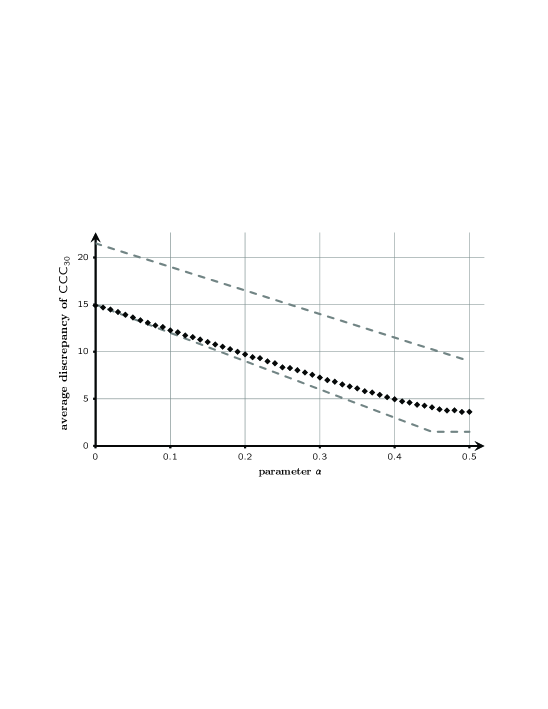
6. Experimental Result

We examined experimentally how well a $\mathsf{CCC}$ balances a random input. We implemented a $\mathsf{CCC}_{2^{30}}$ consisting of roughly one billion wires and thirty billion balancers. The input was chosen independently uniformly at random from $\{0,1,2,\ldots,2^{30}-1\}$. For initial directions of the balancers all up and different values $\alpha$ between $0$ and $1/2$ we measured the resulted discrepancy.

Figure 2 presents the average over 100 runs, together with theoretical lower and upper bounds. As the input is random, the so-far presented bounds can be tightened. Following the same lines of proof, one can easily show the following slightly better bounds on the expected discrepancy $\Delta$ in the random-input case:

• $\Delta\leqslant(\frac{1}{2}-\alpha)\cdot(\log n-\lceil\log\log n\rceil)+\lceil\log\log n\rceil+4,$

• $\Delta\geqslant\max\{(1/2-\alpha)\log n,\;1/2\,(1-\tfrac{1}{n})\,(\lfloor\log\log n\rfloor-1)\}$.

As these bounds are only used for visualization in Figure 2 and the proofs are very similar to the above, they are omitted.

References

• Arthur and Vassilvitskii [2006] D. Arthur and S. Vassilvitskii. Worst-case and smoothed analysis of the icp algorithm, with an application to the k-means method. In 47th IEEE Symp. on Found. of Comp. Science (FOCS’06), pages 153–164, 2006.
• Aspnes et al. [1994] J. Aspnes, M. Herlihy, and N. Shavit. Counting networks. J. of the ACM, 41(5):1020–1048, 1994.
• Bertsekas and Tsitsiklis [1997] D. Bertsekas and J. Tsitsiklis. Parallel and Distributed Computation: Numerical Methods. Athena Scientific, 1997.
• Bohman et al. [2003] T. Bohman, A. Frieze, and R. Martin. How many random edges make a dense graph hamiltonian? Random Structures and Algorithms, 22(1):33–42, 2003.
• Coja-Oghlan et al. [2009] A. Coja-Oghlan, U. Feige, A. M. Frieze, M. Krivelevich, and D. Vilenchik. On smoothed $k$-CNF formulas and the walksat algorithm. In 20th ACM-SIAM Symp. on Discrete Algorithms (SODA’09), pages 451–460, 2009.
• Dowd et al. [1989] M. Dowd, Y. Perl, L. Rudolph, and M. Saks. The periodic balanced sorting network. J. of the ACM, 36(4):738–757, 1989.
• Feige [2007] U. Feige. Refuting smoothed 3CNF formulas. In 48th IEEE Symp. on Found. of Comp. Science (FOCS’07), pages 407–417, 2007.
• Flaxman and Frieze [2007] A. Flaxman and A. Frieze. The diameter of randomly perturbed digraphs and some applications. Random Structures and Algorithms, 30:484–504, 2007.
• Friedrich and Sauerwald [2009] T. Friedrich and T. Sauerwald. Near-perfect load balancing by randomized rounding. In 41st Annual ACM Symposium on Theory of Computing (STOC’09), pages 121–130, 2009.
• Friedrich et al. [2009] T. Friedrich, T. Sauerwald, and D. Vilenchik. Smoothed analysis of balancing networks. In 36th International Colloquium on Automata, Languages, and Programming (ICALP’09), volume 5556 of Lecture Notes in Computer Science, pages 472–483. Springer, 2009.
• Herlihy and Shavit [2008] M. Herlihy and N. Shavit. The Art of Multiprocessor Programming. Morgan Kaufmann, 2008.
• Herlihy and Tirthapura [2006a] M. Herlihy and S. Tirthapura. Randomized smoothing networks. J. Parallel and Distributed Computing, 66(5):626–632, 2006a.
• Herlihy and Tirthapura [2006b] M. Herlihy and S. Tirthapura. Self-stabilizing smoothing and counting networks. Distributed Computing, 18(5):345–357, 2006b.
• Krivelevich et al. [2006] M. Krivelevich, B. Sudakov, and P. Tetali. On smoothed analysis in dense graphs and formulas. Random Structures and Algorithms, 29(2):180–193, 2006.
• Manthey and Reischuk [2007] B. Manthey and R. Reischuk. Smoothed analysis of binary search trees. Theoret. Computer Sci., 378(3):292–315, 2007.
• Mavronicolas and Sauerwald [2008] M. Mavronicolas and T. Sauerwald. The impact of randomization in smoothing networks. In 27th Annual ACM Principles of Distributed Computing (PODC’08), pages 345–354, 2008.
• Rabani et al. [1998] Y. Rabani, A. Sinclair, and R. Wanka. Local divergence of Markov chains and the analysis of iterative load balancing schemes. In 39th Annual IEEE Symposium on Foundations of Computer Science (FOCS’98), pages 694–705, 1998.
• Röglin and Vöcking [2007] H. Röglin and B. Vöcking. Smoothed analysis of integer programming. Math. Program., 110(1):21–56, 2007.
• Spielman and Teng [2004] D. Spielman and S. Teng. Smoothed analysis of algorithms: Why the simplex algorithm usually takes polynomial time. J. of the ACM, 51(3):385–463, 2004.
• Vershynin [2006] R. Vershynin. Beyond hirsch conjecture: Walks on random polytopes and smoothed complexity of the simplex method. In 47th IEEE Symp. on Found. of Comp. Science (FOCS’06), pages 133–142, 2006.