New type of parametrizations for parton distributions

Abstract

New type of parametrization for parton distribution functions, based on an exact their $Q^{2}$-evolution at large and small $x$ values, is constructed for valence quarks. It preserves exactly the low $x$ and large $x$ asymptotics of the solution of the DGLAP equation and obeys the Gross-Llewellyn-Smith sum rule.

I Introduction

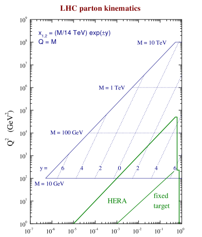
The parton distribution functions (PDFs) which contribute to the LHC processes, and the PDFs fitted at HERA and fixed target experiments are defined at somewhat different $(x,Q^{2})$ ranges (see, for example, Fig. 1 taken from Thorne2005 ). Therefore, a direct application of the modern PDF sets NNLOfits to the LHC processes is not well justified.

This problem is really important, because the larger uncertainties for many processes at the LHC originate mainly from our restricted knowledge of the parton distributions (see, for example, the recent paper Forte and references therein).

In the present paper we propose an idea to overcome this problem. Our solution consists of the two basic steps. Firstly, we find asymptotics of solutions of the Dokshitzer-Gribov-Lipatov-Altarelli-Parisi (DGLAP) equations DGLAP for the parton densities at low and large $x$ values of the Bjorken variable and, at the next step, we approach a combination of the two solutions for the full range of $x$.

In a sense, this is not a new idea. A similar approach had been given by the Spanish group (see book Yndu and references therein) about 40 years ago. However, in the present paper the parametrization will be constructed in a rather different way. In particular, it includes an important subasymptotic term which is fixed exactly by the sum rules.

The results of the present paper are restricted by the leading order (LO) of the perturbation expansion, what is reasonable Sherstnev , since for many processes at the LHC the next-to-leading-order (NLO) corrections are not known so far. Moreover, in the present study we limit ourselves to the valence quarks, whose evolution does not contain contributions from the gluons.

Figure 1: The $(x,Q^{2})$ ranges of the PDFs contributed to the LHC processes and ones fitted at HERA and fixed target experiments (from Thorne2005 ).

II A short theoretical input

In this section we briefly present the theoretical part of our analysis. The reader is referred to Kotikov2007 for more details.

The deep-inelastic scattering (DIS) $l+N\to l^{\prime}+X$, where $l$ and $N$ are the incoming lepton and nucleon, and $l^{\prime}$ is the outgoing lepton, in the one of basic processes to study of the nucleon structure. The DIS cross-section can be split to the lepton $L^{\mu\nu}$ and hadron $F^{\mu\nu}$ parts

$$d\sigma\sim L^{\mu\nu}F^{\mu\nu}\,.$$ (1)

The lepton part $L^{\mu\nu}$ is evaluated exactly, while the hadron one, $F^{\mu\nu}$, can be presented in the following form

$$F^{\mu\nu} = \left(-g^{\mu\nu}+\frac{q^{\mu}q^{\nu}}{q^{2}}\right)\,F_{1}(x,Q^{2})$$ (2)

$$+ \left(p^{\mu}+\frac{(pq)}{q^{2}}q^{\mu}\right)\left(p^{\nu}+\frac{(pq)}{q^{2}}q^{\nu}\right)\,F_{2}(x,Q^{2})$$

$$+ i\varepsilon_{\mu\nu\alpha\beta}p^{\alpha}p^{\beta}\frac{x}{q^{2}}\,F_{3}(x,Q^{2})+\dots\,,$$

where the symbol $\dots$ stands for the parts, which depend on the nucleon spin. The functions $F_{k}(x,Q^{2})$ (hereafter $k=1,2,3$) are the DIS structure functions (SFs) and $q$ and $p$ are the photon and parton momenta. Moreover, the two variables

$$Q^{2}=-q^{2}>0~{},~{}~{}x=\frac{Q^{2}}{2(pq)}$$ (3)

determine the basic properties of the DIS process. Here, $Q^{2}$ is the “mass” of the virtual photon and/or $Z/W$ boson, and the Bjorken variable $x$ ($0<x<1$) is the part of the hadron momentum carried by the scattering parton (quark or gluon).

II.1 Mellin transform

The Mellin transform diagonalizes the $Q^{2}$ evolution of the parton densities. In other words, the $Q^{2}$ evolution of the Mellin moment with certain value $n$ does not depend on the moment with another value $n^{\prime}$.

The Mellin moments $M_{k}(n,Q^{2})$ of the SF $F_{k}(x,Q^{2})$

$$M_{k}(n,Q^{2})=\int_{0}^{1}dx\,\,x^{n-1}F_{k}(x,Q^{2})$$ (4)

can be represented as the sum

$$M_{k}(n,Q^{2})=\sum_{a=q,\bar{q},G}\,C^{a}_{k}(n,Q^{2}/\mu^{2})\,A_{a}(n,\mu^{2}),$$ (5)

where $C^{a}_{k}(n,Q^{2}/\mu^{2})$ are the coefficient functions and $A_{a}(n,\mu^{2})=<N|\mathcal{O}^{a}_{\mu_{1},...,\mu_{n}}|N>$ are the matrix elements of the Wilson operators $\mathcal{O}^{a}_{\mu_{1},...,\mu_{n}}$, which in turn are process independent.

Phenomenologically, the matrix elements $A_{a}(n,\mu^{2})$ are equal to the Mellin moments of the PDFs $f_{a}(x,\mu^{2})$, where $f_{a}(x,\mu^{2})$ are the parton distributions of quarks ($a=q_{i}$), antiquarks ($a=\bar{q}_{i}$) with $(i=1,\cdots,6$), and gluons ($a=G$), i.e.

$$A_{a}(n,\mu^{2})\equiv f_{a}(n,\mu^{2})=\int_{0}^{1}dx\,\,x^{n-1}f_{a}(x,\mu^{2})\,.$$ (6)

The coefficient functions $C^{a}_{k}(n,Q^{2}/\mu^{2})$ are represented by

$$C^{a}_{k}(n,Q^{2}/\mu^{2})=\int_{0}^{1}dx\,\,x^{n-1}\tilde{C}^{a}_{k}(x,Q^{2}/\mu^{2})$$ (7)

and responsible for the relationship between SFs and PDFs. Indeed, in the $x$-space the relation (5) is replaced by

$$F_{k}(x,Q^{2})=\sum_{a=q,\bar{q},G}\,\tilde{C}^{a}_{k}(x,Q^{2}/\mu^{2})\otimes f_{a}(x,\mu^{2})\,,$$ (8)

where $\otimes$ denotes the Mellin convolution

$$f_{1}(x)\otimes f_{2}(x)\equiv\int^{1}_{x}\,\frac{dy}{y}\,f_{1}(y)f_{2}\left(\frac{x}{y}\right)\,.$$ (9)

Using Eqs. (5) and (8), one can fit the shapes of PDFs $f_{a}(x,\mu^{2})$, which are process-independent and use them later on for another processes. Indeed, the cross-sections of the hadron-hadron processes are proportional to the parton luminosities $f_{a,b}(x,\mu^{2})$ (see, for example, the recent paper Neubert and references therein), which are the Mellin convolutions of the two PDFs $f_{a}(x,\mu^{2})$ and $f_{b}(x,\mu^{2})$:

$$f_{a,b}(x,\mu^{2})=f_{a}(x,\mu^{2})\otimes f_{b}(x,\mu^{2})\,.$$ (10)

II.2 Quark distribution functions

The distributions of the $u$ and $d$ quarks contain the valence and the sea parts

$$f_{q_{1}}\equiv f_{u}=f_{u}^{V}+f_{u}^{S}~{},~{}~{}f_{q_{2}}\equiv f_{d}=f_{d}^{V}+f_{d}^{S}\,.$$ (11)

The distributions of the other quark flavors and of all the antiquarks contain the sea parts only:

$$f_{q_{j}}=f_{q_{j}}^{S},~{}~{}(j=3,4,5,6),~{}~{}~{}f_{\bar{q}_{i}}=f_{\bar{q}_{i}}^{S}~{}~{}(i=1,\cdots,6)\,.$$ (12)

It is useful to define the combinations of quark densities, the valence part $f_{V}$, the sea one $f_{S}$ and the singlet one $f_{SI}$ Buras

$$f_{V} = f_{u}^{V}+f_{d}^{V}~{},~{}~{}f_{S}=\sum_{i=1}^{6}\left(f_{q_{i}}^{S}+f_{\bar{q}_{i}}^{S}\right)~{},$$

$$f_{SI} = \sum_{i=1}^{6}\left(f_{q_{i}}+f_{\bar{q}_{i}}\right)=f_{V}+f_{S}\,.$$ (13)

Because the PDFs, which contribute to the structure functions, are accompanied by some numerical factors, there are also nonsinglet parts

$$f_{\Delta_{ij}}=\left(f_{q_{i}}+f_{\bar{q}_{i}}\right)-\left(f_{q_{j}}+f_{\bar{q}_{j}}\right)\,,$$ (14)

which contain difference of densities of quarks and antiquarks with different values of charges.

As an example, we consider the electron-proton scattering, where the corresponding SF has the form

$$F_{2}^{ep}(x,Q^{2})=\sum_{i=1}^{6}e_{i}^{2}\left(f_{q_{i}}(x,Q^{2})+f_{\bar{q}_{i}}(x,Q^{2})\right)\,.$$ (15)

In the four-quark case (when $b$ and $t$ quarks are separated out), as in Buras , we will have

$$F_{2}^{ep}(x,Q^{2})=\frac{5}{18}\,f_{SI}(x,Q^{2})+\frac{1}{6}f_{\Delta}(x,Q^{2})\,,$$ (16)

where

$$f_{\Delta} =\sum_{q_{i}=u,c}\left(f_{q_{i}}(x,Q^{2})+f_{\bar{q}_{i}}(x,Q^{2})\right)$$

$$-\sum_{q_{i}=d,s}\left(f_{q_{i}}(x,Q^{2})+f_{\bar{q}_{i}}(x,Q^{2})\right)\,.$$ (17)

II.3 DGLAP equation

The PDFs obey the DGLAP equation DGLAP

$$\frac{d}{d\ln{\mu^{2}}}\,f_{a}(x,\mu^{2})~{}=\sum_{b}\tilde{\gamma}_{ab}(x)\otimes f_{b}(x,\mu^{2})\,,$$ (18)

where $a,b=NS,SI,G$ and $\tilde{\gamma}_{ab}(x)$ are the so-called splitting functions.

Anomalous dimensions $\gamma_{ab}(n)$ of the twist-two Wilson operators $\mathcal{O}^{a}_{\mu_{1},...,\mu_{n}}$ in the brackets $b$ are the Mellin transforms of the corresponding splitting functions

$$\gamma_{ab}(n)=\int_{0}^{1}dx\,\,x^{n-1}\tilde{\gamma}_{ab}(x)\,.$$ (19)

In the Mellin moment space, the DGLAP equation becomes to be the standard renormalization-group equation

$$\frac{d}{d\ln{\mu^{2}}}\,f_{a}(n,\mu^{2})~{}=\sum_{b=NS,SI,G}\tilde{\gamma}_{ab}(n)\,f_{b}(n,\mu^{2})\,.$$ (20)

Below we will study the properties of the valence part only. Consideration of the other quark densities will be discussed separately.

III Low and large $x$ asymptotics

The large $x$ asymptotics of the valence quark density has the following form Gross ; LoYn

$$f_{V}(x,Q^{2})~{}\to~{}B_{V}(s)(1-x)^{\beta_{V}(s)}\,,$$ (21)

where

$$s=\ln\left(\frac{\ln(Q_{0}^{2}/\Lambda^{2})}{\ln(Q^{2}/\Lambda^{2})}\right)\,,~{}\beta_{V}(s)=\beta_{V}(0)+\hat{d}_{V}s\,,~{}\hat{d}_{V}=\frac{16}{3\beta_{0}}\,,$$

$$B_{V}(s)=B_{V}(0)\frac{e^{-p_{V}s}}{\Gamma(1+\beta_{V}(s))}\,,~{}p_{V}=\hat{d}_{V}\left(\gamma_{E}-\frac{3}{4}\right)s\,.$$ (22)

$B_{V}(0)$ and $\beta_{V}(0)$ are free parameters. Here $\beta_{0}=11-2f/3$ is the first term of the QCD $\beta$-function, $f$ is the number of active quarks and $\gamma_{E}$ is the Euler constant. The constant $\beta_{V}(0)$ can be estimated from the quark counting rules schot as

$$\beta_{V}(0)\sim 3\,.$$ (23)

Eqs. (21) and (22) demonstrate the fall of the parton densities at large $x$ values when $Q^{2}$ increases.

At small-$x$ values the valence part has the following asymptotics FMartin ; LoYn ; Kotikov1993

$$f_{V}(x)~{}\to~{}A_{V}(s)\,x^{\lambda_{V}}\,,$$ (24)

where

$$A_{V}(s)=A_{V}(0)e^{-d_{NS}(1-\lambda_{V})s}\,,$$ (25)

$$d_{NS}(n)=\frac{16}{3\beta_{0}}\left[\Psi(n+1)+\gamma_{E}-\frac{3}{4}-\frac{1}{2n(n+1)}\right]\,.$$

$\lambda_{V}$ and $A_{V}(0)$ are free parameters and $\Psi(n+1)$ is Euler $\Psi$-function.

From the Regge calculus the constant $\lambda_{V}\sim 0.3\div 0.5$. Moreover, the $Q^{2}$ evolution of this parton density shows that $\lambda_{V}$ should be $Q^{2}$ independent Kotikov1996 .

In Eq. (25) the “anomalous dimension” $d_{NS}(n)$ is represented in the form which is useful for the non-integer $n$ values. Usually, the elements of the coefficient functions and anomalous dimensions are expressed as the combinations of the nested sums Vermaseren , which can be expanded, however, to the non-integer $n$ values according to KaKo .

IV Parametrization

The valence quark part $f_{V}(x,Q^{2})$ can be represented in the following form

$$f_{V}(x,Q^{2})=x^{\lambda_{V}}(1-x)^{\beta_{V}(s)}\biggl{[}A_{V}(s)(1-x)+B_{V}(s)x\biggr{]}\,,$$ (26)

which is constructed as a combination of the small $x$ and large $x$ asymptotics, the last term is equal to $A_{V}(s)$ at small $x$ and to $B_{V}(s)$ at large $x$ values. The $Q^{2}$-dependence of the parameters in (26) is given by Eqs. (22) and (25).

IV.1 Gross-Llewellyn-Smith sum rule

The additional relation between the parameters in (26) stems from the LO Gross-Llewellyn-Smith sum rule GrLl

$$\int_{0}^{1}\frac{dx}{x}f_{V}(x,Q^{2})=Q_{V}~{},~{}~{}Q_{V}=3\,,$$ (27)

which simply informs about the number of the valence quarks in nucleon.

As long as the Eq. (26) is just a parametrization, an attempt to apply the sum rule for, e.g., $k$ different values of $Q^{2}$ produces $k$ additional relations that is, of course, unacceptable. The sum rule can be applied only at one point $s=s_{C}$ for some critical value of $Q^{2}_{C}$. For the other values of $Q^{2}$, the sum rule holds only approximately and one can estimate the deviation from the exact sum rule.

So, we have the following relation

$$Q_{V} =\frac{\Gamma(\lambda_{V})\Gamma(1+\beta_{V}(s_{C}))}{\Gamma(\lambda_{V}+2+\beta_{V}(s_{C}))}\Bigl{[}\lambda_{V}B_{V}(0)e^{-p_{V}s_{C}}$$

$$+(1+\beta_{V}(s_{C}))A_{V}(0)e^{-d_{NS}(1-\lambda_{V})s_{C}}\Bigr{]}\,.$$ (28)

It is possible to choose any “middle” value of $s$. However, if $s_{C}=0$, i.e. $Q^{2}_{C}=Q^{2}_{0}$, then Eq. (28) is considerably simplified

$$Q_{V}=\frac{\Gamma(\lambda_{V})\Gamma(1+\beta_{V}(0))}{\Gamma(\lambda_{V}+2+\beta_{V}(0))}\Bigl{[}\lambda_{V}B_{V}(0)+(1+\beta_{V}(0))A_{V}(0)\Bigr{]}\,.$$ (29)

IV.2 Subasymptotic term

In the present paper we choose another possibility to take exactly the sum rule (27) into account. We introduce an additional term $\sim D_{V}(s)$ to our parameterization (26), which can be written as

$$f_{V}(x, Q^{2})=x^{\lambda_{V}}(1-x)^{\beta_{V}(s)}$$ (30)

$$\times\Bigl{[}A_{V}(s)(1-x)+B_{V}(s)x+D_{V}(s)\sqrt{x}(1-x)\Bigr{]}\,,$$

where the last term in the brackets is subasymptotic in both the small and the large $x$ values. These types of the subasymptotic reduction, $\sim\sqrt{x}$ at small $x$ and $\sim(1-x)$ at large $x$ values, have been discussed in Yndu .

Now, the sum rule (27) can be satisfied at any $Q^{2}$ values and determines completely the new term,

$$Q_{V} = \frac{\Gamma(\lambda_{V})\Gamma(1+\beta_{V}(s))}{\Gamma(\lambda_{V}+2+\beta_{V}(s))}\,\Bigl{[}\lambda_{V}B_{V}(s)+(1+\beta_{V}(s))A_{V}(s)\Bigr{]}$$ (31)

$$+ \frac{\Gamma(\lambda_{V}+1/2)\Gamma(2+\beta_{V}(s))}{\Gamma(\lambda_{V}+5/2+\beta_{V}(s))}\,D_{V}(s)\,.$$

V Results

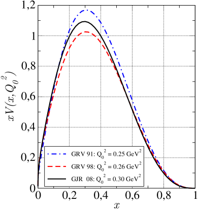
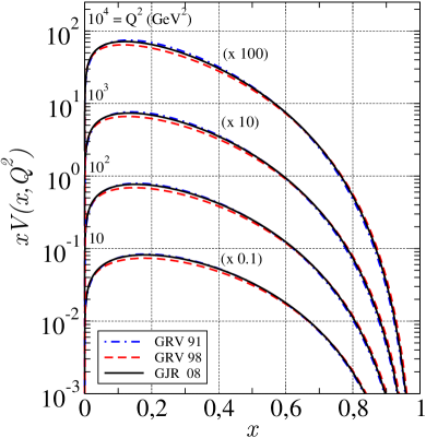
To obtain the parameters of our parameterization (30) for the valence part, we compare it numerically with the results of several Gluck-Reya-Vogt (GRV) sets GRV92 ; GRV98 and Gluck-Jimenez-Delgado-Reya (GJR) one GRV08 . The choice of the GRV/GJR evolution is related to future investigations of the gluon and sea quark densities; the small $x$ asymptotics obtained in Q2evo are conceptually close to the GRV/GJR approach.

	$f$	$\alpha_{s}(M_{Z})$	$Q_{0}^{2}~{}(\mbox{GeV}^{2})$	$A_{V}(0)$	$B_{V}(0)$	$\lambda_{V}$	$\beta_{V}(0)$
GRV(1991) GRV92	4	0.1282	0.25	0.61	80.62	0.317	2.870
GRV(1998) GRV98	3	0.1250	0.26	0.93	64.80	0.333	2.812
GJR(2008) GRV08	3	0.1263	0.30	1.07	85.60	0.390	2.945

Table 1: The parameters of the valent quark distribution of Eq. (30) fitted on several GRV/GJR sets.

With the parameters, reported in the Table 1 our parameterization (30) and the GRV/GJR sets are in good agreement for all $x$ values in the very broad $Q^{2}$ range, $0.25$ GeV² $<Q^{2}<10^{4}$ GeV².

Then, the parameterization (30) describes the experimental data as well as the GRV/GJR sets and has the analytic form containing the exact asymptotics (21) and (24) of the DGLAP evolutions at small and large $x$ values. Thus, it can be applied with good warranty in any other ($x,Q^{2}$) region, where the experimental data are still not available. So, it should be applicable for the LHC range of $x$ and $Q^{2}$ values.

Note, that all GRV/GJR sets themselves give quite close results for the valence quarks, i.e. these results should not change significantly when the new data will appear, for example, from the LHC experiments.

Figure 2: The valence quark density at $Q^{2}_{0}$.

Figure 3: The valence quark density at several values of $Q^{2}$: $Q^{2}=10^{m}$ GeV² with $m=1,2,3$ and $4$.

VI Conclusions

In this work, we investigated the low $x$ and large $x$ asymptotics of the valence quark density, and obtained the corresponding parametrization (30). This parametrization obeys explicitly the Gross-Llewellyn-Smith sum rule. It has been compared with various GRV/GJR sets GRV92 ; GRV98 ; GRV08 in order to fit the initial values of all the $Q^{2}$-dependent parameters. It has been performed accurately, because numerically the form (30) and the GRV/GJR sets have very similar shapes for all $x$ and $Q^{2}$ values.

At the next step, we plan to add to our analysis the nonsinglet and sea quark densities as well as the gluon distribution, and apply the obtained results to the analysis of several LHC processes. Moreover, a comparison of these results with the predictions of other sets NNLOfits of the parton densities will be done. We also plan to consider the PDFs in nuclei. Therefore, the EMC effect EMC , which is very important in the high-energy regime, will be added to the consideration.

VII Acknowledgements

We are grateful to Zaza Merebashvili and Igor Cherednikov for careful reading the text and to the authors of GRV08 for the correspondence. The work was supported by RFBR grant No.10-02-01259-a.

Calculations were partially performed on the HPC facility of SISSA/Democritos in Trieste and partially on the HPC facility “WIGLAF” of the Department of Physics, University of Trento.