Supernova, baryon acoustic oscillations, and CMB surface distance constraints on $f(G)$ higher order gravity models

Abstract

We consider recently proposed higher order gravity models where the action is built from the Einstein-Hilbert action plus a function $f(G)$ of the Gauss-Bonnet invariant. The models were previously shown to pass physical acceptability conditions as well as solar system tests. In this paper, we compare the models to combined data sets of supernovae, baryon acoustic oscillations, and constraints from the CMB surface of last scattering. We find that the models provide fits to the data that are close to those of the LCDM concordance model. The results provide a pool of higher order gravity models that pass these tests and need to be compared to constraints from large scale structure and full CMB analysis.

I introduction

Higher order gravity models have been proposed among possible causes of late-time cosmic acceleration HOGpapers . These models are built out of higher order curvature invariants that yield generalized field equations with a coupling between the mass content of the universe and the space-time curvature that produces a late-time self accelerating phase. A large body of papers have been devoted to the so-called $f(R)$ FRpapers models while a smaller fraction study models based on invariants built out of the Ricci and Riemann tensors RicciRiemannpapers .

In addition to the phenomenology of an accelerating cosmic expansion, higher-order gravity models have theoretical motivations within unification theories of fundamental interactions, and through field quantization on curved space-times BirrellDavies1982 ; Weinberg1995 . Indeed, higher-order invariants appear automatically in most quantum gravity proposals DeWitt1965 ; Ashtekar1981 ; Weinberg1995 , string theories Polshinski19982000 ; GreenSchwarzWitten19871999 , supergravity Brandt2002 ; ChamseddineArnowittNath1982 , and loop quantum gravity/cosmology AshtekarLewandowski2004 ; Rovelli1998 ; DateSengupta2009 . In these theories, high-order loop corrections on curved space-time are related to higher-order combinations of the Riemann curvature invariants. Higher-order invariants have been actively discussed in relation to avoiding cosmological curvature singularities (see SingularityPapers and references therein). In some of these theories, the invariants are regrouped in a topological invariant combination called the Gauss-Bonnet invariant, denoted as $G$. This combination gives a theory free of unphysical states DeWitt1965 ; Zwiebach1985 ; LiBarrowMota2007 .

In this paper, we study cosmological constraints on some models where the action is made of the Einstein-Hilbert action plus a function $f(G)$ of the Gauss-Bonnet invariant. We focus on models that have been shown in previous literature to be free of ghost instabilities and superluminal propagations GBpapers in cosmological homogeneous and isotropic backgrounds. We perform coordinate transformations in order to write the dynamical equations in a form integrable using numerical schemes and then compare the models to recent observations of supernova magnitude-redshift data, distance to the CMB surface, and Baryon Acoustic Oscillations (BAO), including Hubble Key project and age constraints.

II $f(G)$ models

The models that we investigate in this paper are derived from varying the action

$$I=\int{d^{4}x\sqrt{-g}\left[\frac{1}{2}R+f(G)\right]+\int{d^{4}x}\sqrt{-g}L_{m}}+\int{d^{4}x}\sqrt{-g}L_{rad}$$ (1)

with respect to the metric $\delta g_{\alpha\beta}$, where

$$G=R^{2}-4R^{\alpha\beta}R_{\alpha\beta}+R^{\alpha\beta\gamma\delta}R_{\alpha\beta\gamma\delta}$$ (2)

is the Gauss-Bonnet invariant, $R$ is the Ricci scalar, $R_{\alpha\beta}$ is the Ricci tensor, $R_{\alpha\beta\gamma\delta}$ is the Riemann tensor, $L_{m}$ and $L_{rad}$ are the matter and radiation energy Lagrangians, respectively. We will work in units with reduced Planck mass $M_{pl}^{2}=(8\pi G_{N})^{-1}=1$. The corresponding field equations read

$${8[R_{\alpha\gamma\beta\delta}+R_{\gamma\beta}g_{\delta\alpha}-R_{\gamma\delta}g_{\beta\alpha}-R_{\alpha\beta}g_{\delta\gamma}+R_{\alpha\delta}g_{\beta\gamma}+\frac{1}{2}R(g_{\alpha\beta}g_{\delta\gamma}-g_{\alpha\delta}g_{\beta\gamma})]\nabla^{\gamma}\nabla^{\delta}}f_{G}$$

$$+\,(Gf_{G}-f)g_{\alpha\beta}+R_{\alpha\beta}-\frac{1}{2}g_{\alpha\beta}R=T_{\alpha\beta},$$ (3)

where we use the definition $f_{G}\equiv\frac{\partial{f}}{\partial{G}}$.

Now using the Friedmann-Lemaitre-Robertson-Walker flat metric

$$ds^{2}=-dt^{2}+a(t)^{2}d\vec{x}^{2}$$ (4)

and Universe filled with matter and radiation, one derives the generalized Friedmann equation

$$3H^{2}=Gf_{G}-f{G}-24H^{3}\dot{f}_{G}+\rho_{m}+\rho_{rad}.$$ (5)

where $\rho_{m}$ and $\rho_{rad}$ are the matter and radiation energy densities, respectively, $H=\dot{a}/a$ and a dot represents $d/dt$. We also note that in terms of $H$,

$$R=6(\dot{H}+2H^{2})$$ (6)

and

$$G=24H^{2}(\dot{H}+H^{2}).$$ (7)

We explore explicit models in the next sections.

III Recently proposed viable $f(G)$ models

III.1 $f(G)$ models proposed by De Felice and Tsujikawa

In Ref. DeFelice2008 , the authors imposed certain conditions on the function $f(G)$ and its derivatives. The most important condition being $d^{2}f/dG^{2}>0$ in order to ensure the stability of a late-time de Sitter solution as well as the existence of a radiation/matter dominated epochs preceding a late-time accelerating phase. Other additional regularity and viability conditions in DeFelice2008 single out the following $f(G)$ functions

Model DFT-A: $$f(G)=\lambda\frac{G}{\sqrt{G_{0}}}\arctan\Big{(}\frac{G}{G_{0}}\Big{)}-\frac{\lambda}{2}\sqrt{G_{0}}\ln{\Big{(}1+\frac{G^{2}}{G_{0}^{2}}\Big{)}}-\alpha\lambda\sqrt{G_{0}},$$ (8)

Model DFT-B: $$f(G)=\lambda\frac{G}{\sqrt{G_{0}}}\arctan\Big{(}\frac{G}{G_{0}}\Big{)}-\alpha\lambda\sqrt{G_{0}},$$ (9)

Model DFT-C: $$f(G)=\lambda\sqrt{G}\ln{\Big{[}\cosh\Big{(}\frac{G}{G_{0}}\Big{)}\Big{]}}-\alpha\lambda\sqrt{G_{0}},$$ (10)

where $\lambda$, $G_{0}$ and $n$ are positive constants and $\alpha$ is a constant. These functions were derived from the integration of the following second order derivatives that satisfy the condition $f_{,GG}>0$ for all values of $G$ along with other regularity conditions DeFelice2008 .

Model DFT-A: $$f_{,GG}=\frac{\lambda}{G_{0}^{3/2}[1+(G^{2}/G_{0}^{2})^{n}]},\,\,n=1$$ (11)

Model DFT-B: $$f_{,GG}=\frac{2\lambda}{G_{0}^{3/2}[1+(G^{2}/G_{0}^{2})^{n}]},\,\,n=2$$ (12)

Model DFT-C: $$f_{,GG}=\frac{\lambda}{G_{0}^{3/2}}[1-\tanh^{2}(G/G_{0})],$$ (13)

Varying the corresponding actions with respect to the metric, the generalized Friedmann equations follow as:

Model DFT-A:

$$3H^{2}=-\sqrt{G_{0}}\Big{(}1152H^{6}(H(4H^{\prime}+3H+H^{\prime\prime})-\alpha(H+H^{\prime})^{2})$$ (14)

$$-576H^{6}\ln{\Big{(}1+\frac{G^{2}}{G_{0}^{2}}\Big{)}}(H+H^{\prime})^{2}-\ln{\Big{(}1+\frac{G^{2}}{G_{0}^{2}}\Big{)}}G_{0}^{2}-2\alpha G_{0}^{2}\Big{)}\lambda\Big{/}2(G_{0}^{2}+G^{2})$$

$$+\frac{3H_{0}^{2}\Omega_{m}}{e^{3N}}+\frac{3H_{0}^{2}\Omega_{rad}}{e^{4N}}+\Lambda,$$

Model DFT-B:

$$3H^{2}=\Big{(}\alpha G_{0}^{4}-576G_{0}^{2}H^{6}(H^{\prime}+H)(5H^{\prime}+H)+1152\alpha G_{0}^{2}H^{6}(H^{\prime}+H)^{2}$$ (15)

$$+331776H^{12}(H^{\prime}+H)^{4}(1+\alpha)\Big{)}\sqrt{G_{0}}\lambda\Big{/}(G_{0}^{2}+G^{2})^{2}+\frac{3H_{0}^{2}\Omega_{m}}{e^{3N}}+\frac{3H_{0}^{2}\Omega_{rad}}{e^{4N}}+\Lambda,$$

Model DFT-C:

$$3H^{2}=\lambda\Big{(}24\sinh\Big{(}\frac{G}{G_{0}}\Big{)}G_{0}H^{3}\cosh\Big{(}\frac{G}{G_{0}}\Big{)}(H^{\prime}+H)$$ (16)

$$-576H^{6}(3H^{\prime 2}-H(4H^{\prime}+H^{\prime\prime}))$$

$$+G_{0}^{2}\cosh\Big{(}\frac{G}{G_{0}}\Big{)}^{2}\Big{(}\alpha-\ln\Big{(}\cosh\Big{(}\frac{G}{G_{0}}\Big{)}\Big{)}\Big{)}\Big{)}\Big{/}G_{0}^{(3/2)}\cosh\Big{(}\frac{G}{G_{0}}\Big{)}^{2}$$

$$+\frac{3H_{0}^{2}\Omega_{m}}{e^{3N}}+\frac{3H_{0}^{2}\Omega_{rad}}{e^{4N}}+\Lambda,$$

where $\Lambda=\alpha\lambda\sqrt{G_{0}}$ and we define $N=\ln{a}$ with ${}^{\prime}=d/dN$. As discussed in Mena2006 ; MoldenhauerIshak2009 , these higher order gravity models have generalized Friedmann equations that are very stiff ordinary differential equations (ODEs) that require us to use well-adapted numerical codes and logarithmic variables. Thus, we replaced $H$ in the ODEs by the logarithmic variable $u=\ln{(H/\hat{\mu})}$ where $\hat{\mu}$ is a constant normalizing the Hubble parameter. This allows one to write the source terms, see Mena2006 , as

$$\tilde{u}=\ln{(\tilde{\omega}_{rad}e^{-4N}+\tilde{\omega}_{m}e^{-3N})}/2$$ (17)

and

$$\tilde{\omega}_{m}\equiv\frac{8\pi G}{3}\frac{\rho_{0}}{\hat{\mu}^{2}}.$$ (18)

Further, with $\omega_{m}=\Omega_{m}h^{2}$ and $h=H_{0}/(100km/s/Mpc)$, one writes

$$\tilde{\omega}_{m}=\frac{\omega_{m}}{\hat{\mu}^{2}}.$$ (19)

Similarly, $\tilde{\omega}_{rad}$ is defined for radiation but we consider its contribution to be negligible at late times.

In terms of the logarithmic variables, the generalized Friedmann equations (equations (14) (15) (16)) may be written

Model DFT-A: $$(e^{2u}-H_{\Lambda}^{2})(\hat{\mu}^{2}(G_{0}^{2}+G(u)^{2}))-\frac{1}{6}\sqrt{G_{0}}\lambda\Big{(}(G_{0}^{2}+G(u)^{2})\ln\Big{(}\frac{G_{0}^{2}+G(u)^{2}}{G_{0}^{2}}\Big{)}$$ (20)

$$-1152\hat{\mu}^{8}e^{8u}(4u^{\prime}(u^{\prime}+1)+u^{\prime\prime})\Big{)}=0,$$

Model DFT-B: $$(e^{2u}-H_{\Lambda}^{2})(3\hat{\mu}^{2}(G_{0}^{2}+G(u)^{2})^{2})-G(u)^{4}$$ (21)

$$+576\hat{\mu}^{8}e^{8u}G_{0}^{2}\Big{(}(7u^{\prime}-1)(u^{\prime}+1)+2u^{\prime\prime}\Big{)}=0,$$

Model DFT-C: $$(e^{2u}-H_{\Lambda}^{2})-\frac{\sqrt{G_{0}}\lambda}{3\hat{\mu}}\Big{(}\frac{-576\hat{\mu}^{8}e^{8u}(4u^{\prime}(u^{\prime}+1))+u^{\prime\prime})}{G_{0}^{2}\cosh^{2}{\Big{(}\frac{G(u)}{G_{0}}}\Big{)}}$$ (22)

$$+\frac{G(u)}{G_{0}}\tanh{\Big{(}\frac{G(u)}{G_{0}}\Big{)}}-\ln\Big{[}\cosh{\Big{(}\frac{G(u)}{G_{0}}\Big{)}}\Big{]}\Big{)}=0,$$

where $H_{\Lambda}^{2}=(\tilde{\omega}_{r}e^{-4N}+\tilde{\omega}_{m}e^{-3N})+\frac{\Lambda}{3\hat{\mu}^{2}}$ and $G(u)=\hat{\mu}^{4}e^{4u}24(u^{\prime}+1)$.

Unlike equations (14), (15), and (16), we found that the equations written in terms of the logarithmic variables allow stable numerical integrations over redshift ranges from $z=5$ to $z=0$. As discussed in MoldenhauerIshak2009 , it is necessary to perform the integration forward in time (backward in the redshift) with initial conditions provided by some approximate solutions at high redshift. We verified that at higher redshifts ($z>5$), the approximate solutions provide an excellent fit to the numerical solution of the ODEs with a relative difference $\frac{H_{approx}-H(z)}{H(z)}$ that is better than $0.1\%$. We use these approximations in order to find the numerical initial conditions for $u$ and $u^{\prime}$ at $z=5$ and then start a numerical integration of the ODEs down to the supernovae locations. Proceeding in this way, we obtained very stable programs to derive various Hubble plots for the HOG models. The approximate solutions for the models of this section can be derived as

Model DFT-A: $$H^{2}=\hat{\mu}^{2}H_{\Lambda}^{2}+\frac{\sqrt{G_{0}}\lambda}{6(G_{0}^{2}+G(\tilde{u})^{2})}\Big{(}(G_{0}^{2}+G(\tilde{u})^{2})\ln\Big{(}\frac{G_{0}^{2}+G(\tilde{u})^{2}}{G_{0}^{2}}\Big{)}$$ (23)

$$-1152\hat{\mu}^{8}e^{8\tilde{u}}(4\tilde{u}^{\prime}(\tilde{u}^{\prime}+1)+\tilde{u}^{\prime\prime})\Big{)},$$

Model DFT-B: $$H^{2}=\hat{\mu}^{2}H_{\Lambda}^{2}+\frac{G(\tilde{u})^{4}-576\hat{\mu}^{8}e^{8\tilde{u}}G_{0}^{2}\Big{(}(7\tilde{u}^{\prime}-1)(\tilde{u}^{\prime}+1)+2\tilde{u}^{\prime\prime}\Big{)}}{3(G_{0}^{2}+G(\tilde{u})^{2})^{2}},$$ (24)

Model DFT-C: $$H^{2}=\hat{\mu}^{2}H_{\Lambda}^{2}+\frac{\sqrt{G_{0}}\lambda}{3}\Big{(}\frac{-576\hat{\mu}^{8}e^{8\tilde{u}}(4\tilde{u}^{\prime}(\tilde{u}^{\prime}+1))+\tilde{u}^{\prime\prime})}{G_{0}^{2}\cosh^{2}{\Big{(}\frac{G(\tilde{u})}{G_{0}}}\Big{)}}$$ (25)

$$+\frac{G(\tilde{u})}{G_{0}}\tanh{\Big{(}\frac{G(\tilde{u})}{G_{0}}\Big{)}}-\ln\Big{[}\cosh{\Big{(}\frac{G(\tilde{u})}{G_{0}}\Big{)}}\Big{]}\Big{)},$$

where $G(\tilde{u})=\hat{\mu}^{4}e^{4\tilde{u}}24(\tilde{u}^{\prime}+1)$ and the source $\tilde{u}$ is used from earlier.

The generalized Friedmann equations above along with their high redshift approximations are in a form ready for numerical integration and comparisons to observational data in §4.

III.2 $f(G)$ models proposed by Zhou, Copeland and Saffin

The authors of ZhouCopeland2009 performed a thorough phase space analysis of $f(G)$ models and analyzed some specific models that satisfy some cosmological viability conditions. Following Amendola2006 for $f(R)$ models, the authors of ZhouCopeland2009 expressed the viability conditions as constraints on the derivatives of the function $f(G)$. We consider here some of their models as:

Model ZCS-A: $$f(G)=\alpha\sqrt{G}+\beta\sqrt[4]{G},$$ (26)

Model ZCS-B: $$f(G)=\alpha(G^{3/4}-\beta)^{2/3},$$ (27)

Model ZCS-C: $$f(G)=\sqrt{\alpha}\exp(\beta/G).$$ (28)

where $\alpha$ and $\beta$ are constants. The equations of motion in a flat FLRW spacetime follow as:

Model ZCS-A:

$$3H^{2}=-\Big{(}\frac{1}{2}\alpha\sqrt{G}H(H^{3}-\frac{1}{2}(H^{\prime 2}H+H^{\prime\prime}H^{2}))$$ (29)

$$+\frac{3}{4}\beta\sqrt[4]{G}H(\frac{1}{2}H^{\prime 2}H+H^{3}+H^{2}H^{\prime}-\frac{1}{4}(H^{\prime 2}H+H^{\prime\prime}H^{2}))\Big{)}\Big{/}\Big{(}H^{\prime}H+H^{2}\Big{)}$$

$$+\frac{3H_{0}^{2}\Omega_{m}}{e^{3N}}+\frac{3H_{0}^{2}\Omega_{rad}}{e^{4N}}$$

Model ZCS-B:

$$3H^{2}=\frac{1}{2}\alpha\Big{(}2(H^{2}(H^{\prime}H+H^{2}))^{3/4}\beta^{3}H(H^{\prime}+H)-576H^{12}(H^{\prime}+H)24^{1/4}$$ (30)

$$-\frac{1}{2}H^{4}(9H^{\prime 2}+18H^{\prime}H+10H^{2})(H^{2}(H^{\prime}H+H^{2}))^{1/2}24^{3/4}$$

$$+12\beta H^{7}(5H^{\prime 3}+15H+18H^{\prime}H^{2}+8H^{2})(H^{2}(H^{\prime}H+H^{2}))^{1/4}24^{1/2}$$

$$+\Big{(}288H^{9}(H^{\prime}+H)^{2}24^{1/4}+\frac{1}{4}H^{3}\beta^{2}(H^{2}(H^{\prime}H+H^{2}))24^{3/4}$$

$$-18H^{6}\beta(H^{\prime}+H)(H^{2}(H^{\prime}H+H^{2}))^{1/4}24^{1/2}\Big{)}(H^{\prime 2}H+H^{\prime\prime}H^{2})\Big{)}\Big{/}$$

$$\Big{(}(H^{\prime}H+H^{2})(24^{3/4}(H^{2}(H^{\prime}H+H^{2}))^{3/4}-\beta)^{7/3}(H^{2}(H^{\prime}H+H^{2}))^{3/4}\Big{)}$$

$$+\frac{3H_{0}^{2}\Omega_{m}}{e^{3N}}+\frac{3H_{0}^{2}\Omega_{rad}}{e^{4N}}$$

Model ZCS-C:

$$3H^{2}=-\alpha\exp\Big{(}\frac{\beta}{24H^{2}/(H^{\prime}H+H^{2})}\Big{)}\Big{(}(288H^{10}(H^{\prime}+H)^{2}+2\beta^{2}H^{2}H^{\prime}(H^{\prime}+2H)$$ (31)

$$+(H^{\prime 2}H+H^{\prime\prime}H^{2})(24H^{4}\beta(H^{\prime}+H)+\beta^{2}H-144H^{7}(H^{\prime}+H)^{2}))(24H^{3}H^{\prime}+24H^{4})^{1/2}$$

$$+24H^{5}\beta(H^{3}+9H^{\prime 2}H+7H^{\prime}H^{2}+3H^{\prime 3})\Big{)}\Big{/}\Big{(}576H^{4}(H^{\prime}H+H^{2})^{4}\Big{)}$$

$$+\frac{3H_{0}^{2}\Omega_{m}}{e^{3N}}+\frac{3H_{0}^{2}\Omega_{rad}}{e^{4N}}$$

Again, in order to compare these models to cosmological data, we must write the generalized Freidmann equation in a numerically stable integrable form using logarithmic variables yielding:

Model ZCS-A:

$$(e^{2u} - e^{2\tilde{u}})(48\hat{\mu}^{2}(u^{\prime}+1)^{2})-4\alpha\sqrt{G(u)}(u^{\prime\prime}+2(u^{\prime}+1)(u^{\prime}-1))$$ (32)

$$-3\beta\sqrt[4]{G(u)}(u^{\prime\prime}-4(u^{\prime}+1))=0,$$

Model ZCS-B:

$$(e^{2u}-e^{2\tilde{u}})6\hat{\mu}^{2}(u^{\prime}+1)(G(u)(G(u)^{3/4}-\beta)^{7/3})-(G(u)^{13/4}(u^{\prime}-1)$$ (33)

$$+G(u)^{5/2}\beta(u^{\prime}+4)-G(u)^{7/4}\beta^{2}(4u^{\prime}+5)+2G(u)\beta^{3}(u^{\prime}+1))$$

$$-6\hat{\mu}^{4}e^{4u}(2G(u)^{9/4}-3G(u)^{3/2}\beta+G(u)^{3/4}\beta^{2})u^{\prime\prime}=0,$$

Model ZCS-C:

$$(e^{2u}-e^{2\tilde{u}})(3\hat{\mu}^{2}(u^{\prime}+1)^{2}G(u)^{2})+\alpha\sqrt{G(u)}\exp(\beta/G(u))\Big{(}\Big{(}-\frac{1}{2}G(u)^{2}(u^{\prime}-1)$$ (34)

$$+G(u)\beta(5u^{\prime}+1)+4\beta^{2}u^{\prime}\Big{)}(u^{\prime}+1)+\Big{(}\beta^{2}-\frac{1}{4}G(u)^{2}+G(u)\beta\Big{)}u^{\prime\prime}\Big{)}=0,$$

We also need the approximate solution for these models at high redshift providing initial conditions for numerical integrations as discussed in previous section. The approximate solutions at high redshift for these models are:

Model ZCS-A:

$$H^{2}=\hat{\mu}^{2}e^{2\tilde{u}}+\frac{4\alpha\sqrt{G(\tilde{u})}(\tilde{u}^{\prime\prime}+2(\tilde{u}^{\prime}+1)(\tilde{u}^{\prime}-1))+3\beta\sqrt[4]{G(\tilde{u})}(\tilde{u}^{\prime\prime}-4(\tilde{u}^{\prime}+1))}{48(\tilde{u}^{\prime}+1)^{2}},$$ (35)

Model ZCS-B:

$$H^{2} = \hat{\mu}^{2}e^{2\tilde{u}}+\Big{(}(G(\tilde{u})^{13/4}(\tilde{u}^{\prime}-1)+G(\tilde{u})^{5/2}\beta(\tilde{u}^{\prime}+4)-G(\tilde{u})^{7/4}\beta^{2}(4\tilde{u}^{\prime}+5)$$ (36)

$$+2G(\tilde{u})\beta^{3}(\tilde{u}^{\prime}+1))+6\hat{\mu}^{4}e^{4\tilde{u}}(2G(\tilde{u})^{9/4}-3G(\tilde{u})^{3/2}\beta$$

$$+G(\tilde{u})^{3/4}\beta^{2})\tilde{u}^{\prime\prime}\Big{)}\Big{/}\Big{(}6\hat{\mu}(G(\tilde{u})^{3/4}-\beta)^{7/3}G(\tilde{u})(\tilde{u}^{\prime}+1)\Big{)},$$

Model ZCS-C:

$$H^{2} = \hat{\mu}^{2}e^{2\tilde{u}}+\alpha\sqrt{G(\tilde{u})}\exp(\beta/G(\tilde{u}))\Big{(}\Big{(}-\frac{1}{2}G(\tilde{u})^{2}(\tilde{u}^{\prime}-1)+G(\tilde{u})\beta(5\tilde{u}^{\prime}+1)+4\beta^{2}\tilde{u}^{\prime}\Big{)}(\tilde{u}^{\prime}+1)$$ (37)

$$+\Big{(}\beta^{2}-\frac{1}{4}G(\tilde{u})^{2}+G(\tilde{u})\beta\Big{)}\tilde{u}^{\prime\prime}\Big{)}\Big{/}\Big{(}3\hat{\mu}^{2}(\tilde{u}^{\prime}+1)^{2}G(\tilde{u})^{2}\Big{)},$$

where again $G(\tilde{u})=\hat{\mu}^{4}e^{4\tilde{u}}24(\tilde{u}^{\prime}+1)$ and the source $\tilde{u}$ is as defined earlier.

III.3 $f(G)$ Models proposed by Uddin, Lidsey and Tavakol

The models presented by Uddin2009 are similar to the models presented by ZhouCopeland2009 of the previous section, i.e. $f(G)=\alpha\sqrt{G}+\beta\sqrt[4]{G}$, with $\beta=0$ and $\alpha=\sqrt{4\alpha}$, although Uddin2009 performed a different and independent analysis. In agreement with the analogous scalar field models, the power-law form of the $f(G)$ model as $f(G)=\pm 2\sqrt{\alpha G}$ was found to have stable scaling solutions. The authors studied the equation of state parameter for these models as it evolved through radiation, matter and accelerating epochs. The behavior of the energy densities were also discussed there. By investigating stability for both vacuum and non-vacuum solutions, it was recognized that those models suffered from a singular point at transition. Our results for these models can be found with results for the ZCS models in §5 below.

Figure 1: LEFT: $2D$ joint contour plots for DFT-A with parameters $\Omega_{m}$, $\alpha$, $\lambda$, $\hat{\mu}$, $H_{0}$ for Union, WMAP5 and SDSS LRG(BAO) data sets, where the inner and outer loops are $68\%$ and $95\%$, respectively. RIGHT:$2D$ joint contour plots for DFT-A with parameters $\Omega_{m}$, $\alpha$, $\lambda$, $G_{0}$, $H_{0}$ for Union, WMAP5 and SDSS LRG(BAO) data sets, where the inner and outer loops are $68\%$ and $95\%$, respectively.

IV Cosmological distances constraints from SNe Ia, CMB surface, and BAO

In this section, we describe the three cosmological observations used to constrain the models described above. One of the first compelling evidences for cosmic acceleration came from the Supernovae type Ia (SNe Ia) observations and we use here the distance modulus as a function of the redshift $z$ given by

$$\mu(z)=\tilde{m}-M=5\log{D_{L}}+25$$ (38)

containing the magnitude-redshift function, $\tilde{m}(z)$ and a nuisance parameter, $M$ which is degenerate with the Hubble parameter, $H_{0}$. The luminosity distance, $D_{L}$ in units of Mpc for HOG models is given by

$$D_{L}(z)=(1+z)\int^{z}_{0}\frac{1}{H(z^{\prime})}dz^{\prime}\,,$$ (39)

with $H(z^{\prime})$ as the solution to the non-linear differential equations given above for the higher order gravity models (recall that for the logarithmic variables defined in the previous section the redshift reads as $z=e^{-N}-1$.) We use the Union set of supernovae which was compiled as an attempt to gather the best of the best supernovae from different surveys, including Supernovae Legacy Survey, ESSENCE Survey, HST, and other older sets Kowalski2008 . After selection cuts, the 414 SNe Ia are reduced to 307. The fitting of the SNe Ia uses a standard minimization method, $\chi^{2}$,

$$\chi_{SN}^{2}=\sum^{i=307}_{i=1}\frac{[\mu^{i}_{HOG}(z)-\mu^{i}_{obs}(z)]^{2}}{\sigma^{2}}$$ (40)

where $\sigma$ is the magnitude uncertainty and $i$ the number of data points compared. We break degeneracies in the parameter space by using the value of the Hubble parameter as measured by the Hubble Key Project (HST)HubbleKeyProject , $H_{0}=72\pm 8\,km/s/Mpc$.

Next, we consider the distance to the CMB last scattering surface and, following Komatsu2008 , we define three fitting parameters for comparison to the WMAP5 data using the shift parameter, $R$, see for example Bond ,

$$R(z_{*})=\sqrt{\Omega_{m}}H_{0}(1+z_{*})D_{A}(z_{*}),$$ (41)

with the redshift, $z_{*}$ for the surface of last scattering, see for example HuSugiyama ,

$$z_{*}=1048[1+0.00124(\Omega_{b}h^{2})^{-0.738}][1+g_{1}(\Omega_{m}h^{2})^{g_{2}}],$$ (42)

where

$$g_{1}=\frac{0.0783(\Omega_{b}h^{2})^{-0.238}}{1+39.5(\Omega_{b}h^{2})^{0.763}},$$ (43)

and

$$g_{2}=\frac{0.560}{1+21.1(\Omega_{b}h^{2})^{1.81}},$$ (44)

and third, the acoustic scale, $l_{a}$, is, see for example WangMukherjee ; Wright ,

$$l_{a}=(1+z_{*})\frac{\pi D_{A}(z_{*})}{r_{s}(z_{*})},$$ (45)

with the proper angular diameter distance, $D_{A}(z)=D_{L}(z)/(1+z)^{2}$ and the comoving sound horizon, $r_{s}(z_{*})$, see for example Percival2007 ,

$$r_{s}(z_{*})=\frac{1}{\sqrt{3}}\int^{1/(1+z_{*})}_{0}{\frac{da}{a^{2}H(a)\sqrt{1+(3\Omega_{b}/4\Omega_{\gamma})a}}},$$ (46)

with $\Omega_{\gamma}=2.469\times 10^{-5}h^{-2}$ for $T_{cmb}=2.725K$.

Figure 2: LEFT: $2D$ joint contour plots for DFT-B with parameters $\Omega_{m}$, $\alpha$, $\lambda$, $G_{0}$, $H_{0}$ for Union, WMAP5 and SDSS LRG(BAO) data sets, where the inner and outer loops are $68\%$ and $95\%$, respectively. RIGHT:$2D$ joint contour plots for DFT-C with parameters $\Omega_{m}$, $\alpha$, $\lambda$, $G_{0}$, $H_{0}$ for Union, WMAP5 and SDSS LRG(BAO) data sets, where the inner and outer loops are $68\%$ and $95\%$, respectively.

Together the parameters $x_{i}=(R,l_{a},z_{*})$ are used to fit $\chi^{2}_{WMAP}=\triangle x_{i}Cov^{-1}(x_{i}x_{j})\triangle x_{j}$ with $\triangle x_{i}=x_{i}-x^{obs}_{i}$ and $Cov^{-1}(x_{i}x_{j})$ is the inverse covariance matrix for the parameters.

Thirdly, we use BAO constraints following Komatsu2008 ; Percival2007 ; Eisenstein2005 ; Tegmark and defining the ratio of the sound horizon, $r_{s}(z_{d})$ to the effective distance, $D_{V}$ as a fit for SDSS by

$$\chi^{2}_{BAO}=\Big{(}\frac{r_{s}(z_{d})/D_{V}(z=0.2)-0.198}{0.0058}\Big{)}^{2}+\Big{(}\frac{r_{s}(z_{d})/D_{V}(z=0.35)-0.1094}{0.0033}\Big{)}^{2},$$ (47)

with, see for example Eisenstein2005 ,

$$D_{V}(z)=\Big{(}D_{A}^{2}(z)(1+z)^{2}\frac{z}{H(z)}\Big{)}^{1/3},$$ (48)

and the redshift, $z_{d}$ as, see for example EisensteinHu1998 ,

$$z_{d}=\frac{1291(\Omega_{m}h^{2})^{0.251}}{1+0.659(\Omega_{m}h^{2})^{0.828}}[1+b_{1}(\Omega_{b}h^{2})^{b_{2}}],$$ (49)

where

$$b_{1}=0.313(\Omega_{m}h^{2})^{-0.419}[1+0.607(\Omega_{m}h^{2})^{0.674}],$$ (50)

and

$$b_{2}=0.238(\Omega_{m}h^{2})^{0.223}.$$ (51)

We use a modified and extended version of the publicly available package, CosmoMC cosmomc to perform a Monte Carlo Markov Chain analysis (MCMC’s). The MCMC’s are used to compute the likelihoods for the parameters in the model. This method randomly chooses values for the above parameters and, based on the $\chi^{2}$ obtained, either accepts or rejects the set of parameters via the Metropolis-Hastings algorithm. When a set of parameters is accepted it is added to the chain and forms a new starting point for the next step. The process is repeated until the specified convergence is reached. We found that an elaborate and essential step in our analysis was to numerically integrate the stiff ODEs in order to derive the Hubble expansion rate for a wide range of redshift and integrate it to the CosmoMC package. For this task, we made a necessary change of variable in our integration and also used a good approximation at higher redshifts in order to obtain initial values for our codes to perform stable integrations from $z=5$ down to $z=0$. We used the framework developed to compare the models described in the previous sections to the three sets of observations and the results are given in the next section.

Figure 3: LEFT: $2D$ joint contour plots for ZCS-A with parameters $\Omega_{m}$, $\alpha$, $\beta$, $H_{0}$ for Union, WMAP5 and SDSS LRG(BAO) data sets, where the inner and outer loops are $68\%$ and $95\%$, respectively. CENTER:$2D$ joint contour plots for ZCS-B with parameters $\Omega_{m}$, $\alpha$, $\beta$, $H_{0}$ for Union, WMAP5 and SDSS LRG(BAO) data sets, where the inner and outer loops are $68\%$ and $95\%$, respectively. RIGHT:$2D$ joint contour plots for ZCS-C with parameters $\Omega_{m}$, $\alpha$, $\beta$, $H_{0}$ for Union, WMAP5 and SDSS LRG(BAO) data sets, where the inner and outer loops are $68\%$ and $95\%$, respectively.

V Results and Conclusion

Figure 4: Comparisons of different SNe Ia plots with Union data and different values of $f(G)$ models. LEFT: Comparison of DFT-A, DFT-B, DFT-C Models and LCDM. RIGHT:Comparison of ZCS-A, ZCS-B, ZCS-C Models and LCDM.

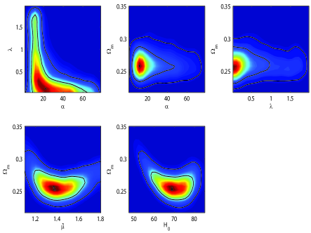
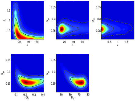
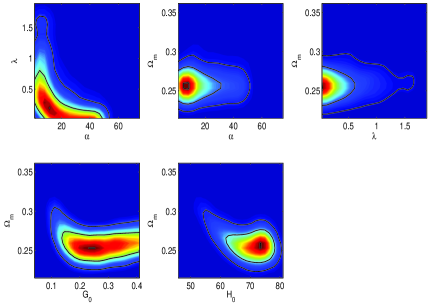
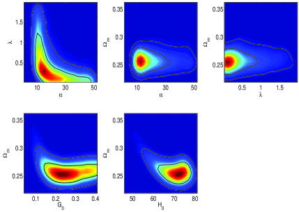
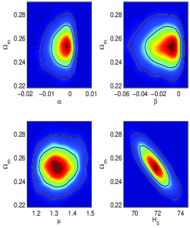
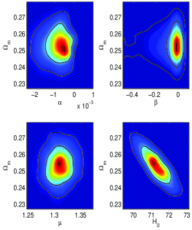
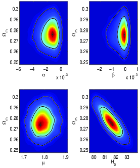
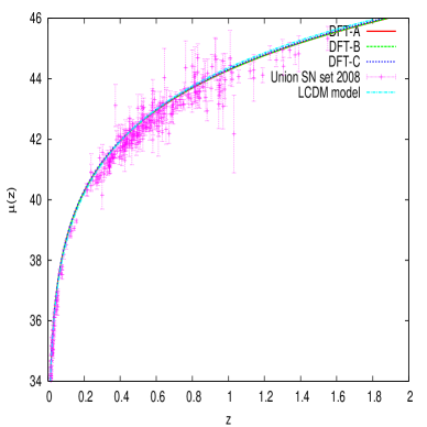
Our results are summarized in figures 1-4 and in table I. In figure 1, we present the results for model DFT-A. We first (left part of figure 1) varied $\Omega_{m}$, $\alpha$, $\lambda$, $\hat{\mu}$, and $H_{0}$ leaving $G_{0}\sim h^{4}$ as a derived parameter, and we obtained a normalized $\chi^{2}/dof=1.0754$ ($\chi^{2}=329.1$). On the right part of figure 1 for model DFT-A, we varied $\Omega_{m}$, $\alpha$, $\lambda$, $G_{0}$, and $H_{0}$ leaving $\hat{\mu}$ as a derived parameter, with a normalized $\chi^{2}/dof=1.0751$ ($\chi^{2}=329.0$). Our best fit values are given in table 1 and we find an $\Omega_{m}$ around $0.25$ in both cases. We find best values for the model parameters $\alpha$ and $\lambda$ that have a product $\alpha\lambda$ of the order unity as required, see DeFelice2008 . We find the best fit for $\hat{\mu}$ that is of the order of twice the normalized Hubble parameter $h$, as it should Mena2006 ; MoldenhauerIshak2009 , and the best fit parameter $G_{0}$ of the order of $h^{4}$ DeFelice2008 . Next, we show in figure 2 the results for models DFT-B and DFT-C with similar results and normalized $\chi^{2}/dof=1.0764$ ($\chi^{2}=329.4$) and $\chi^{2}/dof=1.0748$ ($\chi^{2}=328.9$) respectively. Finally, we show in figure 3, results for the ZCS models varying the parameters $\alpha$, $\beta$, $\hat{\mu}$, $\Omega_{m}$ and $H_{0}$.

Constraints from	$\chi^{2}$	$\chi^{2}/dof$	$\Omega_{m}$	$H_{0}$	$\hat{\mu}$	$G_{0}$	$\alpha$	$\lambda$	$\beta$
Observations
$DFT-A$	$329.1$	$1.0754$	$0.254939^{+0.049835}_{-0.025707}$	$71.2827^{+11.8991}_{-17.8981}$	$1.4424^{+0.356636}_{-0.309619}$	$-$	$26.6096^{+48.3636}_{-21.5027}$	$0.136131^{+1.75928}_{-0.111111}$	$-$
$DFT-A$	$329.0$	$1.0751$	$0.253516^{+0.0607013}_{-0.0231282}$	$68.1122^{+11.3855}_{-16.2845}$	$-$	$.214908^{+0.194690}_{-0.114864}$	$54.3437^{+20.6530}_{-44.9701}$	$0.0832318^{+1.81255}_{-0.058080}$	$-$
$DFT-B$	$329.4$	$1.0764$	$0.251225^{+0.0537648}_{-0.0218609}$	$70.6107^{+8.94104}_{-17.1149}$	$-$	$.253771^{+0.155822}_{-0.149289}$	$9.99891^{+39.9510}_{-6.78136}$	$0.313781^{+1.49185}_{-0.288712}$	$-$
$DFT-C$	$328.9$	$1.0748$	$0.253603^{+0.049532}_{-0.023303}$	$69.6979^{+9.64599}_{-16.0135}$	$-$	$.238717^{+0.170843}_{-0.135459}$	$13.9569^{+36.0160}_{-4.56533}$	$0.529189^{+1.36409}_{-0.473996}$	$-$
$ZCS-A$	$328.2$	$1.0725$	$0.25047^{+0.02857}_{-0.02093}$	$72.066^{+1.6351}_{-2.1441}$	$1.35273^{+0.13186}_{-0.18860}$	$-$	$0.00084^{+0.00016}_{-0.01632}$	$-$	$-0.03498^{+0.03595}_{-0.02399}$
$ZCS-B$	$362.4$	$1.1843$	$0.254855^{+0.018011}_{-0.025755}$	$71.1289^{+1.81457}_{-1.37513}$	$1.30822^{+0.0448309}_{-0.0363830}$	$-$	$-0.00014^{+0.000083}_{-0.001439}$	$-$	$0.00031^{+0.03288}_{-0.76993}$
$ZCS-C$	$332.4$	$1.0862$	$0.27302^{+0.02810}_{-0.01934}$	$81.511^{+1.8530}_{-1.7468}$	$1.7754^{+0.10141}_{-0.07048}$	$-$	$-0.00012^{+0.000004}_{-0.00295}$	$-$	$-0.0000017^{+0.00012}_{-0.00142}$

Table 1: $\chi^{2}$, $\chi^{2}/dof$, and best-fit parameters for $f(G)$ higher order gravity models using observational constraints from supernovae, HST, CMB surface and BAO. For models DFT-A, DFT-B, DFT-C the parameters are $\Omega_{m}$, $H_{0}$, $\hat{\mu}$, $G_{0}$, $\alpha$, and $\lambda$. For models ZCS-A, ZCS-B, ZCS-C the parameters are $\Omega_{m}$, $H_{0}$, $\hat{\mu}$, $\alpha$, and $\beta$.

The best fit parameters are given in table 1. The first and second models have best fit values similar to the DFT models while the third model has slightly higher values for $\Omega_{m}$ and $H_{0}$. The best fit $\chi^{2}$’s for $f(G)$ models are close to the $\chi_{SN+BAO+CMB}^{2}\approx 314.6$ ($\chi^{2}/dof=1.018$) that we obtained for the LCDM concordance model. In view of the of the possible systematic uncertainties in the supernova data, it is not clear that the difference between the $\chi^{2}$s is significant. It is worth noting that the parameter space that we found for the DFT models is also all contained within the parameter space found by DeFeliceSolar for the models to be compatible with solar system constraints. In other words, the DFT models analyzed in this paper pass physical acceptability conditions DeFelice2008 ; DeFelice2009 , solar system tests DeFeliceSolar and here pass constraints from supernova, BAO rulers and distance to CMB last scattering surface. Recently, Ref. DeFeliceMota2009 pointed out in a preliminary work that matter perturbations in Gauss-Bonnet models exhibit some instabilities during the matter era, and that for the growth to be compatible with observations the deviations from general relativity have to be very small. This point needs further investigations using perturbation studies in $f(G)$ models. In view of the success of $f(G)$ models with solar system tests and cosmological distances constraints, we conclude that these models need to be subjected, in future projects, to full large scale structure constraints such as galaxy clustering and gravitational lensing, as well as the full CMB analysis.