Strict inequalities of critical probabilities on Gilbert’s continuum percolation graph
Abstract
Any infinite graph has site and bond percolation critical probabilities satisfying . The strict version of this inequality holds for many, but not all, infinite graphs.
In this paper, the class of graphs for which the strict inequality holds is extended to a continuum percolation model. In Gilbert’s graph with supercritical density on the Euclidian plane, there is almost surely a unique infinite connected component. We show that on this component . This also holds in higher dimensions.
1 Introduction
Consider an infinite connected graph and perform bond percolation by independently marking each edge open with probability and closed otherwise. The critical probability refers to the value of above which there exists almost surely (a.s.) an infinite connected subgraph of , of open edges. Similarly, one can perform site percolation by independently marking each vertex of open with probability and refer to as the critical probability above which there exists a.s. an infinite connected subgraph of , of open vertices.
The weak inequality can easily be proven by dynamic coupling, see for example Chapter 2 of Franceschetti and Meester (2007). If is a tree, then it is also easy to see that , as each vertex, other than some arbitrarily selected root, can be uniquely identified by an edge and vice versa. By adding finitely many edges to an infinite tree, one can also construct other connected graphs for which the equality holds.
On the other hand, the strict inequality has also been shown to hold in several circumstances. Grimmett and Stacey (1998) proved it for a large class of ‘finitely transitive’ graphs including the -dimensional hypercubic lattices.
These graphs, however, do not include the random graphs constructed using continuum percolation models, because they are not ‘finitely transitive’: since their average node degree is not bounded, the group action defined by their automorphisms has infinitely many orbits almost surely. These continuum percolation graphs are the focus of this paper. They are of particular interest in the context of communication networks and are treated extensively in the books by Franceschetti and Meester (2007), Meester and Roy (1996), and Penrose (2003).
We consider Gilbert’s graph, which is defined as follows. Let and let be a homogeneous Poisson point process in of intensity . Gilbert’s graph, here denoted , has as its vertex set the point set , and the edges are obtained by connecting every pair of points such that , by an undirected edge. It is well known that there exists a critical density value , such that if then there exists a.s. a unique infinite connected component, while if then there is a.s no infinite connected component; see e.g. Meester and Roy (1996). When it exists, we denote this infinite component by .
In the site percolation model on , each vertex is independently marked open with probability , and closed otherwise, and we look for an unbounded connected component in the induced subgraph of the open vertices. It is easy to see that this is equivalent to rescaling the original Poisson process to one with intensity and looking for an unbounded connected component there. It follows that for there is a critical value (namely ) such that if then there is a.s. an infinite connected component in , and if then there is a.s. no such infinite component.
In the bond percolation model on , we independently declare each edge to be open with probability , and closed otherwise, and look for an unbounded connected component in the induced subgraph of the open edges. There is a critical probability such that if then there is a.s. an infinite connected component in , and if then there is a.s. no such infinite component. Observe that , and it can also be shown by a branching process comparison that .
Our main result provides strict inequality between and on Gilbert’s graph. Our proof easily extends to or more dimensions.
Theorem 1
Consider for . On we have .
The basic strategy is to adapt the enhancement technique developed for percolation on lattices by Menshikov (1987), Aizenman and Grimmett (1991), Grimmett and Stacey (1998). This consists of constructing an ‘enhanced’ version of the site percolation process for which the critical probability is strictly less than that of the original site process. Then one can use dynamic coupling of the enhanced model with bond percolation to complete the proof.
We face two main difficulties when trying to extend the enhancement technique to a continuum random setting. One of these amounts to constructing the desired enhancement on a random graph rather than on a deterministic one. The second one consists in adapting some basic inequalities for the enhanced graph, given in the discrete setting by Aizenman and Grimmett (1991), to the continuum setting. This requires somehow more involved geometric constructions and a careful incremental build-up of the Poisson point process. Once we circumvent these obstacles, it is not too difficult to obtain the final result using a classic dynamic coupling construction.
The enhancement strategy has been proven useful to show strict inequalities in a variety of contexts: Bezuidenhout, Grimmett, and Kesten (1993), and Grimmett (1994), use this technique in the context of Potts and random cluster models; Roy, Sarkar, and White (1998) use it in the context of directed percolation. In the continuum, Sarkar (1997) uses enhancement to demonstrate coexistence of occupied and vacant phases for the three-dimensional Poisson Boolean model. Roy and Tanemura (2002) use it in the context of percolation of different convex shapes.
2 Proof of Theorem 1
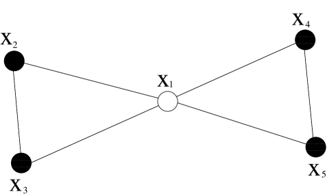
We now describe the enhancement needed to prove Theorem . Throughout this section we consider Gilbert’s graph with . The objective is to describe a way to to add open vertices to the site percolation model to make the probability of an infinite cluster bigger, without changing the bond percolation model. To do so, we introduce two kinds of coloured vertices, red vertices (the original open vertices) and green vertices (closed vertices which have been enhanced) and for any two vertices we write that if they are joined by an edge. In , if we have vertices such that is closed, has no neighbours other than , which are all red, and and but there are no other edges amongst and then we say is correctly configured in , and refer to this as a configuration of edges. If a vertex is correctly configured we make it green with probability , independently of everything else; see Figure 1.
Let be the open disc of radius centred at the origin. Let and be sequences of independent uniform random variables. List the vertices of in order of increasing distance from the origin as . Declare a vertex to be red if and closed otherwise. Once the sets of red and closed vertices have been decided in this way, apply the enhancement by declaring each closed vertex to be green if it is correctly configured and . Whenever we insert a vertex of the Poisson process at , it would have values and associated with it. We shall refer to vertices that are either red or green as being coloured.
Let be the annulus and let be the event that there is a path from a coloured vertex in to a coloured vertex in in using only coloured vertices (note that is based on a process completely inside ; we do not allow vertices outside of to affect possible enhancements inside ).
Let be the probability that occurs, and define
The following proposition states that is indeed the percolation function associated to the enhanced model. From now on we use ‘vertex’ to refer to a point of the Poisson process and ‘point’ to refer to an arbitrary location in .
Proposition 1
There is a.s. an infinite connected component in using only red and green vertices if and only if .
Proof of Proposition 1. For the if part let be the event that there is a coloured path from to outside , so is contained in . Let be the probability of occurring and let be the limit as goes to . Therefore for all so , but is just the probability of there being an infinite coloured component intersecting and it is well known that there is almost surely an infinite coloured component if .
For the only if part, if there is almost surely an infinite component then . Given , we build up the Poisson process on the whole of . If there are any closed vertices that are not definitely correctly or incorrectly configured, we build up the process in the rest of their -neighbourhood, and this determines whether they are green or uncoloured. If any more closed vertices occur they cannot be correctly configured as they will be joined to a closed vertex. Therefore we have built up the process everywhere in a region with , and all uncoloured vertices at this stage will remain uncoloured. Let be the set of coloured vertices that are joined by a coloured path to a coloured vertex in at this stage.
Next, we build out the process radially symmetrically from (apart from where the process has already been built up) until a vertex occurs that is connected to a vertex in . Let be the event that such a vertex occurs at distance between and from the origin, so must occur for to occur. We can find points on the line extended away from the origin such that is from the origin, is from the origin and so on. Surround with circles of radius around them. If there is at least one red vertex in each one of these little circles that is contained in when the process continues to the whole of , and is also red then occurs. Therefore if occurs then the conditional probability of occuring is at least , where
as this is the probability of getting at least one red vertex in each little circle and being red. Therefore for all , so .
Our next lemma provides an analogue of the Margulis-Russo formula for the enhanced continuum model. First, we need to introduce the notion of pivotal vertices.
Given the configuration and inserting a vertex at we say that is - if putting means that occurs but putting means it does not. Notice that can either complete a path (but it cannot do via being enhanced), or it could make another closed vertex correctly configured which in turn would complete a path. We say that is - if inserting a vertex at and putting means occurs but putting means it does not. That is, and adding a closed vertex at means is correctly configured and enhancing it to a green vertex means occurs but otherwise it does not.
For let be the event that is -pivotal in , and set .
Lemma 1
For all and and it is the case that
| (1) |
and
| (2) |
Proof. Let be the -algebra generated by the locations but not the colours of the vertices of . Let be the number of -pivotal vertices. Define -measurable random variables, and as follows; is the conditional probability that occurs, and is the conditional expectation of , given the configuration of . By the standard version of the Margulis-Russo formula for an increasing event defined on a finite collection of Bernoulli variables (Russo (1981), Lemma 3),
Let denote the total number of vertices of in . By the standard coupling of Bernoulli variables, and Boole’s inequality, almost surely, and since is integrable we have by dominated convergence that
| (3) |
and by a standard application of the Palm theory of Poisson processes
(see e.g. Penrose (2003)),
the right hand side of (3)
equals the right hand side
of (1). The proof of (2) is similar.
The key step in proving Theorem is given by the following result.
Lemma 2
There is a continuous function such that for all , and , we have
| (4) |
Before proving this, we give a result saying that we can assume there are only red vertices inside an annulus disk of fixed size. For , and , let be the closed circle (i.e., disk) of radius around , and let denote the annulus . Given and given , let be the event that all vertices in are red.
Lemma 3
Fix and and . There exists a continuous function , such that for all , all and all with or , we have
Proof. We shall consider a modified model, which is the same as the enhanced model but with enhancements suppressed for all those vertices lying in . Let be the event that is 1-pivotal in the modified model.
Returning to the original model, we first create the Poisson process of intensity in , and determine which of these vertices are red. Then we build up the Poisson process of intensity inside and for any of these new vertices with more than neighbours, or with at least one closed neighbour outside , we decide whether they are red or closed. This decides whether or not they are coloured as these vertices cannot possibly become green because they are not correctly configured. We now can tell which of the closed vertices outside are correctly configured, and we determine which of these are green.
This leaves a set of vertices inside that have at most four neighbours. If we surround each vertex in by a circle of radius then we cannot have any point covered by more than of these circles as this means that there is a vertex in with at least neighbours. All of these circles are contained in , which has area . Therefore
For to have any possibility of being -pivotal, at this stage there must be a set contained in such that if every vertex in is coloured and every vertex in is uncoloured then becomes -pivotal. In this case, with probability at least we have every vertex in red and every vertex in closed, which would imply event occurring. Therefore .
Now we note that the occurrence or otherwise of is unaffected by the addition or removal of closed vertices in . This is because the suppression of enhancements in means that these added or removed vertices cannot be enhanced themselves, and moreover any vertices they cause to be correctly or incorrectly configured also cannot be enhanced.
Consider creating the marked Poisson process in , with each Poisson point (vertex) marked with the pair , in two stages. First, add all marked vertices in , and just the red vertices in . Secondly, add the closed vertices in . The vertices added at the second stage have no bearing on the event , so is independent of the event that no vertices at all are added in the second stage. Hence,
with equality if .
Finally, we use a similar argument to the initial argument in this proof. Suppose occurs. Then there exist at most vertices in which are correctly configured for which the possibility of enhancement has been suppressed. If we now allow these to be possibly enhanced, there is a probability of at least that none of them is enhanced, in which case the set of coloured vertices is the same for the modified model as for the un-modified model and therefore occurs. Taking
we are done.
Proof of Lemma 2. As a start, we fix and . We also fix and , and just write for . Define event as before, so that . Also, write for the disk . For now we assume . We create the Poisson process of intensity everywhere on except inside , and decide which of these vertices are red.
Now we create the process of only the red vertices in (a Poisson process of intensity in this region). Assuming there will be no closed vertices in , we then know which of the closed vertices outside are correctly configured, and we determine which of these are green.
Having done all this, let denote the set of current vertices in that are connected to at this stage (by connected we mean connected via a coloured path), and let denote the set of current vertices in that are connected to .
Let be the -neighbourhood of and let be the -neighbourhood of . We build up the red process inwards (i.e., towards from the boundary of ) on until a red vertex occurs (if such a vertex occurs). Set . Suppose (if instead we would reverse the roles of and in the sequel). Then if we say that event has occurred and we let denote an arbitrarily chosen vertex of . Otherwise, we build up the red process inwards on until a red vertex occurs (if such a vertex occurs).
Let be the event that (i) such vertices and occur, and (ii) the sets and are disjoint, and (iii) , and (iv) there is no path from to through coloured vertices in that are not in . If occurs, then must occur.
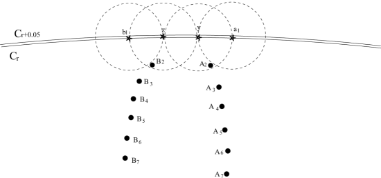
Now suppose has occurred. Let be the point (again we use ‘point’ to refer to a point in ) which is at distance from and distance from on the opposite side of the line to the side is on (see Figure 2). Let be the point lying inside at distance from and from . Let be the circle of radius around . Any red vertex in this circle will be connected to the red vertex (and therefore to a path to ) but cannot be connected to any coloured path to as is the nearest place for such a vertex to be, given occurs. Similarly let be the point lying at distance from and distance from , on the opposite side of to . Then let be the point at distance from and from , and let be the circle of radius around . Any red vertex in will be connected to (and therefore a path to ), but not a path to . Also, any vertex in will be at least away from any vertex in .
Now let be the line through such that and are on different sides of the line and at equal distance from the line. We can pick points such that is within of for , and are both within of but none of the other ’s are within of , and none of the are within of or within of or within of another . Do the same on the other side of with . Now consider circles and of radius around them. Let be the event that there is at exactly one red vertex in each of these circles, and also the circles and , and there are no more new vertices anywhere else in , and no closed vertices in . The probability that occurs, given , is at least
If the events , , occur and then is -pivotal.
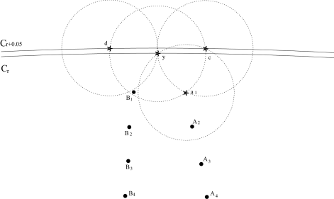
Now we consider the case where occurs but does not, so is inside and is connected to a vertex in that must be outside as is the only vertex in inside (see Figure 3).
Let be the point at distance from and from , on the same side of the line as (assume without loss of generality this is to the right of ). This is the closest can be. Let be the point inside at distance from and from , so this is the furthest left that can be. Let be the point at distance from and from , on the other side of to . Then consider the point inside at distance from and from , and the small circle of radius around . Then any vertex in is distant at least from , and therefore from , as cannot be any nearer than . Also any vertex in will be at least from any other vertices in , as is the nearest place such a point can be. As before we can then have points and with small circles around them such that having one red vertex in each of these vertices ensures that is -pivotal. The probability of getting at least red vertex in each of these circles, a red vertex in and no other new vertices in , and no closed vertices in , is at least .
So by Lemma 3, the probability that is -pivotal satisfies
This proves the claim (4) for the case with .
Now suppose . Then we create the Poisson process in , and decide which of these vertices are red. Then we create the red process in , and determine which vertices in are green, assuming there are no closed vertices in . We then build up the red process in inwards towards until a vertex occurs in the process which is connected to . Let be the event that such a vertex appears at distance between and from , so must occur for to occur.
If is inside we can choose points and such that they are both outside , at distance between and from and at distance between and from each other. We can then choose and such that they are both within of , further than from and and between and from each other. We can then choose points such that is within of for , is within of , no two are within of each other, and no is within of , or , or inside for . Then consider little circles and of radius around these points. If there is at least one red vertex in each of these circles and no vertices anywhere else in then is -pivotal. If is outside we choose points in a similar way but make sure connects with a path to , using little circles which are again of radius and are at least from the . Therefore, setting
and using Lemma 3, we have for some strictly positive continous that
Now suppose . In this case the proof is similar. Again, create the Poisson process in . Then create the red process in and determine which vertices in are green, assuming there are no closed vertices in . Then build the red process in inwards towards until a vertex occurs that is connected to a path of coloured vertices to but not to . Let be the event that such a vertex occurs at distance between and from , and that there is no current coloured path from to , so has to occur for to occur. Given this vertex we can find circles and of radius as before such that having a red vertex in each of these little circles but no other vertices in or ensures is -pivotal. Therefore in this case
Take . By its construction is strictly positive and continuous in and , completing the proof of the lemma.
Proposition 2
There is a continuous function such that
for all and .
Proof of Theorem 1. Set and . Then using Proposition 2 and looking at a small box around , we can find and such that for all we have
Taking the limit inferior as , since is monotone in we get
Now set . Then , so that , and by Proposition 1, the enhanced model with parameters percolates, i.e. has an infinite coloured component, almost surely.
We finish the proof with a coupling argument along the lines of Grimmett and Stacey (1998). Let E be the set of edges and be the set of vertices of (the infinite component). Let and be collections of independent Bernoulli random variables with mean . From these we construct a new collection which constitutes a site percolation process on . Let be an enumeration of the edges of and an enumeration of the vertices. Suppose at some point we have defined for some subset of . Let be the set of vertices not in which are adjacent to some currently active vertex (i.e. a vertex with ). If then let be the first vertex not in and set and add to . If , we let be the first vertex in and let be the first currently active vertex adjacent to it, then set and add to . Repeating this process builds up the entire red site percolation process, if it does not percolate, or a percolating subset of the red site percolation process if it does percolate. In the latter case, the bond process also percolates.
Now suppose the red site process does not percolate. For any correctly configured vertex with up to as before, itself is not red. Therefore at most one edge to has been examined, so we can can find a first unexamined edge (in the enumeration) to or , and then to or . We then declare to be green only if both of these edges are open, which happens with probability . This completes the enhanced site process with and every component in this is contained in a component for the bond process .
Therefore, since the enhanced site process percolates almost surely, so does the bond process, so .
References
- [1]
- [2] M. Aizenman and G. Grimmett (1991). Strict monotonicity for critical points in percolation and ferromagnetic models. J. Statist. Phys. 63, 817–835.
- [3]
- [4] C. Bezuidenhout, G. Grimmett and H. Kesten (1993). Strict inequality for critical values of Potts models and random-cluster processes. Comm. Math. Phys. 158, pp. 1-16.
- [5]
- [6] M. Franceschetti and R. Meester (2007). Random Networks for Communication. Cambridge University Press, Cambridge.
- [7]
- [8] G. Grimmett (1994). Potts models and random-cluster models with many-body interactions. J. Statist. Phys. 75, 67–121.
- [9]
- [10] G. Grimmett and A. Stacey (1998). Critical probabilities for site and bond percolation models. Ann. Probab. 26, 1788–1812.
- [11]
- [12] R. Meester and R. Roy (1996). Continuum Percolation. Cambridge University Press, Cambridge.
- [13]
- [14] M. V. Menshikov (1987). Quantitative estimates and rigorous inequalities for critical points of a graph and its subgraphs. Theory Probab. Appl. 32, 544–547.
- [15]
- [16] M. D. Penrose (2003). Random Geometric Graphs. Oxford University Press, Oxford.
- [17]
- [18] R. Roy, A. Sarkar, and D. White (1998). Backbends in directed percolation. J. Statist. Phys. 91, 889–908.
- [19]
- [20] R. Roy and H. Tanemura (2002). Critical intensities of Boolean models with different underlying convex shapes. Adv. in Appl. Probab. 34, 48–57.
- [21]
- [22] Russo, L. (1981). On the critical percolation probabilities. Z. Wahrsch. Verw. Gebiete 56, 229–237.
- [23]
- [24] Sarkar, A. (1997) Co-existence of the occupied and vacant phase in Boolean models in three or more dimensions. Adv. in Appl. Probab. 29, 878–889.
- [25]