Application of importance sampling to the computation of large deviations in non-equilibrium processes

Abstract

We present an algorithm for finding the probabilities of rare events in nonequilibrium processes. The algorithm consists of evolving the system with a modified dynamics for which the required event occurs more frequently. By keeping track of the relative weight of phase-space trajectories generated by the modified and the original dynamics one can obtain the required probabilities. The algorithm is tested on two model systems of steady-state particle and heat transport where we find a huge improvement from direct simulation methods.

I Introduction

A rare event is one which occurs with a very small probability. However, when they do occur they can have a huge effect and so it is often important to estimate the actual probability of their occurrence. Examples where rare events are important are in banking and insurance, in biological systems where important processes such as genetic switching and mutations occur with extremely small rates, and in nucleation processes. Rare events are also of importance in nonequilibrium processes such as charge and heat transport in small devices and transport in biological cells. The functioning of nano-electronic devices can be affected by rare large-current fluctuations and it is important to know how often they occur.

In this paper our interest is in predicting probabilities of rare fluctuations in transport processes. A number of interesting results have been obtained recently on large fluctuations away from typical behavior in nonequilibrium systems. These include results such as the fluctuation theorems ECM93 ; JW04 ; BD04 ; DDR04 ; DL98 ; visco06 ; SD07 and the Jarzynski relation jarz97 . In the context of transport one typically considers an observable, say $Q$, such as the total number of particles or heat transferred across an object with an applied chemical potential or temperature difference. This is a stochastic variable and for a given observation time $\tau$ this will have a distribution $P(Q,\tau)$. The various general results that have been obtained for $P(Q,\tau)$ give some quantitative measure of the probability of rare fluctuations. Analytic computations of the tails of $P(Q,\tau)$ for any system are usually difficult. This is also true in experiments or in computer simulations since the generation of rare events requires a large number of trials.

For large $\tau$ the probabilities of large fluctuations show scaling behavior $P(Q,\tau)\sim e^{-\tau\,f(Q/\tau)}$, where the function $f(q)$ is known as the large deviation function Varadhan ; Touchette . For a few model systems exact results have been obtained DL98 ; visco06 ; SD07 for either $f(q)$ or its Legendre transform $\mu(\lambda)$, which can be defined in terms of the characteristic function as $\mu(\lambda)=\lim_{\tau\rightarrow\infty}\tau^{-1}\ln\bigl{\langle}e^{-\lambda Q}\bigr{\rangle}$. Recently an algorithm has been proposed GKP06 to compute $\mu(\lambda)$. However, as has been pointed out in Ref. HG09 there may be problems in obtaining the tails of $\mu(\lambda)$ using the algorithm of Ref. GKP06 . The algorithm proposed in this paper is complementary to the one discussed in Ref. GKP06 in the sense that we obtain $P(Q,\tau)$ directly. Our algorithm, based on the idea of importance sampling, computes $P(Q,\tau)$ for any given $\tau$ and accurately reproduces the tails of the distribution. Algorithms based on importance sampling Bucklew have earlier been used in the study of equilibrium systems rosenbluth ; Grassberger:97 and in the study of transition rate processes MJB98 ; dellago98 ; allen05 . However, we are not aware of any applications to the study of large fluctuations of currents in nonequilibrium systems and this is the main focus of this paper. Here we choose two prototype models of transport, namely, heat conduction across a harmonic chain and particle transport in the symmetric simple exclusion process. We illustrate the implementation of importance sampling in the computation of large fluctuations of currents in these two nonequilibrium systems.

Consider a system with a time evolution described by the stochastic process $x(t)$. For simplicity we assume for now that $x(t)$ is an integer-valued variable and time is discrete. Let us denote a particular path in configuration space over a time period $\tau$ by the vector ${\bf x}(\tau):=\{x(t)|t=1,2,\dotsc,\tau\}$ and let $Q$ be an observable which is a function of the path ${\bf x}(\tau)$. We will be interested in finding the probability distribution $P(Q,\tau)$ of $Q$ and especially in computing the probability of large deviations about the mean value $\langle Q\rangle$. As a simple illustrative example consider the tossing of a fair coin. For $\tau=N$ tosses we have a discrete stochastic process described by the time series ${\bf x}(N)=\{x_{i}\}$ where $x_{i}=1$ if the outcome in the $i$th trial is heads and $x_{i}=-1$ otherwise. Suppose we want to find the probability of generating $Q$ heads (thus $Q=\sum_{i=1}^{N}\delta_{x_{i},1}$). An example of a rare event is, for example, the event $Q=N$. The probability of this is $2^{-N}$ and if we were to simulate the coin toss experiment we would need more than $2^{N}$ repeats of the experiment to realize this event with sufficient frequency to calculate the probability reliably. For large $N$ this is clearly very difficult. The importance sampling algorithm is useful in such situations. The basic idea is to increase the occurrence of the rare events by introducing a bias in the dynamics. The rare events are produced with a new probability corresponding to the bias. However, by keeping track of the relative weights of trajectories of the unbiased and biased processes it is possible to recover the required probability corresponding to the required unbiased process.

II The algorithm

We now describe the algorithm in the context of evaluating $P(Q,\tau)$ for the stochastic process ${\bf x}(\tau)$. We denote the probability of a particular trajectory by ${\mathcal{P}}({\bf x})$ . By definition:

$$P(Q,\tau)=\sum_{{\bf x}}\delta_{Q,Q({\bf x})}\mathcal{P}({\bf x}).$$ (1)

For the same system let us consider a biased dynamics for which the probability of the same path ${\bf x}$ is given by ${\mathcal{P}}_{b}({\bf x})$. Then we have:

$$P(Q,\tau) = \sum_{{\bf x}}\delta_{Q,Q({\bf x})}e^{-W({\bf x})}\mathcal{P}_{b}({\bf x}),$$ (2)

$$\text{where}\quad e^{-W({\bf x})} = \frac{\mathcal{P}({\bf x})}{\mathcal{P}_{b}({\bf x})}.$$ (3)

Thus in terms of the biased dynamics, $P(Q,\tau)$ is the average $\langle\delta_{Q,Q({\bf x})}e^{-W}\rangle_{b}$ and in a simulation we estimate this by performing averages over $M$ realizations to obtain:

$$P_{e}(Q,\tau)=\frac{1}{M}\sum_{r}{\delta_{Q,Q({{\bf x}_{r}})}e^{-W({\bf x}_{r})}}~{},$$ (4)

where ${\bf x}_{r}$ denotes the path for the $r$th realization. For $M\to\infty$ we obtain $P_{e}(Q,\tau)\to P(Q,\tau)$ which is the required probability. Note that the weight factor $W$ is a function of the path. In a simulation we know the details of the microscopic dynamics for both the biased and unbiased processes. Thus we can evaluate $W$ for every path ${\bf x}$ generated by the biased dynamics. A necessary requirement of the biased dynamics is that the distribution of $Q$ that it produces [i.e., $P_{b}(Q,\tau)=\langle\delta_{Q,Q({\bf x})}\rangle_{b}$] should be peaked around the desired values of $Q$ for which we want an accurate measurement of $P(Q,\tau)$. As we will see the required dynamics can often be guessed from physical considerations.

We first explain the algorithm for the coin tossing experiment. In this case we consider a biased dynamics where the probability of heads is $p$ and that of tails is $1-p$. If we take $p\approx 1$ then the event $Q=N$, which was earlier rare, is now generated with increased frequency and we can use Eq. (4) to estimate the required probability $P(Q=N,N)$. For any path consisting of $Q$ heads the weight factor is simply given by $e^{-W}=(1/2)^{N}/[p^{Q}(1-p)^{N-Q}]$. Choosing $p=0.95$ it is easy to see that for $N=100$ we can get the required probability $P(Q=N,N)$ with more than $1\%$ accuracy using only $M=10^{7}$ realizations as opposed to at least $M=10^{30}$ required by the unbiased dynamics. Note that for this example $W$ has the same value for all paths with the same $Q$. In general of course $W$ depends on the details of the path, e.g. for a random walk with a waiting probability. We will now illustrate the algorithm with non-trivial examples of computing large deviations in two well known models in nonequilibrium physics. These are the (i) symmetric simple exclusion process (SSEP) with open boundaries and (ii) heat conduction across a harmonic system connected to Langevin reservoirs.

III Symmetric simple exclusion process

This is a well studied example of an interacting stochastic system consisting of particles diffusing on a lattice with the constraint that each site can have at most one particle. Here we restrict ourselves to one-dimension and study the case of an open system where a linear chain with $L$ sites is connected to particle reservoirs at the two ends. The dynamics can be specified by the following rules: (a) a particle at any site $l=1,2,\dotsc,L$ can jump to a neighboring empty site with unit rate; (b) at $l=1$ a particle can enter the system with rate $\alpha$ (if it is empty) and leave with rate $\gamma$. At site $N$ a particle can leave or enter the system with rates $\beta$ and $\delta$, respectively. The biased dynamics can be realized in various ways, for example, by introducing asymmetry in the bulk hopping rates or by changing the boundary hopping rates.

For SSEP, the configuration of the system at any time is specified by the set ${\mathcal{C}}=\{n_{1}(t),n_{1}(t),...,n_{L}(t)\}$ where $n_{l}(t)$ ($0$ or $1$) gives the occupancy of the $l$th site. The dynamical rules specify the matrix element $\mathcal{W}({\mathcal{C}},{\mathcal{C^{\prime}}})$ giving the transition rate from configuration ${\mathcal{C}}^{\prime}$ to ${\mathcal{C}}$. We write $\mathcal{W}({\mathcal{C}},{\mathcal{C^{\prime}}})=\mathcal{W}_{1}+\mathcal{W}_{-1}+\mathcal{W}_{0}$ where $\mathcal{W}_{1}$ and $\mathcal{W}_{-1}$ correspond to transitions whereby a particle enters the system from the left bath or leaves the system into the left bath, respectively, while $\mathcal{W}_{0}$ corresponds to all other transitions. At long times the system will reach a steady state with particles flowing across the system and we are here interested in the current fluctuations in the wire. Specifically, let $Q$ be the net particle transfer from the left reservoir into the system during a time interval $\tau$. For a fixed $\tau$ we want to obtain the distribution $P(Q,\tau)$ of $Q$, in the steady state of the system. It is useful to define the joint probability distribution function $R(Q,\mathcal{C},\tau)$ for $Q$ number of particles transported and for the system to be in state $\mathcal{C}$, given that at $\tau=0$ the system is in the steady state. Clearly $P(Q,\tau)=\sum_{\mathcal{C}}R(Q,\mathcal{C},\tau)$. We also define the characteristic functions $\tilde{R}(z,\mathcal{C},\tau)=\sum_{-\infty}^{\infty}R(Q,\mathcal{C},\tau)z^{Q}$ and $\tilde{P}(z,\tau)=\sum_{\mathcal{C}}\tilde{R}(z,\mathcal{C},\tau)$. It is then easy to obtain the following master equation DDR04 :

$$\frac{d\tilde{R}(z,\mathcal{C},\tau)}{d\tau}=\sum_{\mathcal{C^{\prime}}}\Bigl{[} z\mathcal{W}_{1}(\mathcal{C},\mathcal{C^{\prime}})+\mathcal{W}_{0}(\mathcal{C},\mathcal{C^{\prime}})$$

$$+\frac{1}{z}\mathcal{W}_{-1}(\mathcal{C},\mathcal{C^{\prime}})\Bigr{]}\,\tilde{R}(z,\mathcal{C^{\prime}},\tau).$$ (5)

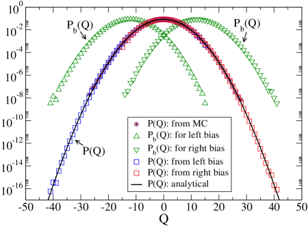
The general solution of this equation for arbitrary $L$ is difficult but for $L=1$ an explicit solution can be obtained for $\tilde{R}(z,\mathcal{C^{\prime}},\tau)$ and $\tilde{P}(z,\tau)$. We will here first discuss a special case $\alpha=\beta=\gamma=\delta$ for which $\tilde{P}(z,\tau)$ can be inverted explicitly. The choice of steady state initial conditions gives the solution: $P(Q,\tau)=({e^{-2\alpha\tau}}/{2})[I_{2Q-1}(2\alpha\tau)+2I_{2Q}(2\alpha\tau)+I_{2Q+1}(2\alpha\tau)]$. In Fig. (1) we plot the exact distribution along with a direct simulation of the above process with averaging over $5\times 10^{8}$ realizations. As we can see the direct simulation is accurate only for events with probabilities of $O(10^{-8})$. Now we illustrate our algorithm using a biased dynamics. We consider biasing obtained by changing the boundary transition rates. We denote the rates of the biased dynamics by $\alpha^{\prime},\beta^{\prime},\gamma^{\prime},\delta^{\prime}$ and these are chosen such that $P_{b}(Q)$ has a peak in the required region. In our simulation we consider a discrete-time implementation of SSEP. For every realization of the process over a time $\tau$ (after throwing away transients) the weight factor $W$ is dynamically evaluated. For instance, every time a particle hops into the system from the left reservoir, $W$ is incremented by $-\ln{(\alpha/\alpha^{\prime})}$. In Fig. (1) we see the result of using our algorithm with two different biases. Using the same number of realizations we are now able to find probabilities up to $O(10^{-16})$ and the comparison with the exact result is excellent.

Figure 1: (Color online) Plot of $P(Q)$ for $\tau=15$ for the one-site SSEP model with $\alpha=\beta=3.0,\gamma=\delta=3.0$. MC refers to direct Monte Carlo simulations. Left bias corresponds to $\alpha^{\prime}=\beta^{\prime}=3.8,\gamma^{\prime}=\delta^{\prime}=2.2$ and right bias to $\alpha^{\prime}=\beta^{\prime}=2.2,\gamma^{\prime}=\delta^{\prime}=3.8$.

Figure 2: (Color online) Plot of $P(Q)$ for $\tau=15$ for the three-site SSEP model with $\alpha=\beta=4.0,\gamma=\delta=2.0$. MC refers to direct Monte Carlo simulations. For left (right) bias simulations, the particles in bulk hop to the left (right) with rate $4$ and to the right (left) with unit rate. The boundary rates are kept unchanged.

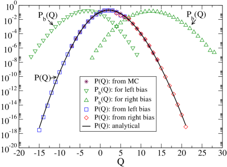
We next study the case with $L=3$ with rates chosen such that the system reaches a nonequilibrium steady state with $\langle Q\rangle>0$. Finding $\tilde{R}(z,\mathcal{C},\tau)$ analytically involves diagonalizing an $8\times 8$ matrix. We do this numerically and after an inverse Laplace transform find $P(Q,\tau)$. In Fig. (2) we show the numerical and direct simulation results for this case and also the results obtained using the biased dynamics; in this case we consider a biased dynamics with asymmetric bulk hopping rates. Again we find that the biasing algorithm significantly improves the accuracy of finding probabilities of rare events using the same number of realizations ($5\times 10^{8}$).

IV Heat conduction

Figure 3: (Color online) Plot of $P(Q)$ for $\tau=200$ for heat conduction across a single free particle with $\gamma_{1}=0.8,\gamma_{2}=0.2,T_{1}=1.1875,T_{2}=0.25$. The parameters have been chosen to correspond to a region in parameter space where the fluctuation theorem is not satisfied visco06 . MC refers to direct Monte Carlo simulations. The left bias corresponds to $\gamma_{1}^{\prime}=\gamma_{1},\gamma_{2}^{\prime}=\gamma_{2}/20,T_{1}^{\prime}=T_{1},T_{2}^{\prime}=20T_{2}$.

Next we consider the problem of heat conduction across a system connected to heat reservoirs modeled by Langevin white-noise reservoirs. Here we are interested in the distribution of the net heat transfer $Q$ from the left bath into the system over time $\tau$. First let us consider the simple example of a single Brownian particle connected to two baths at temperatures $T_{1}$ and $T_{2}$. This model was studied recently by Visco visco06 who obtained an exact expression for the characteristic function of $Q$. The equation of motion for the system is given by:

$$\dot{v}=-(\gamma_{1}+\gamma_{2})v+\sqrt{2D_{1}}\,\eta_{1}+\sqrt{2D_{2}}\,\eta_{2}$$ (6)

where $\eta_{1,2}$ are Gaussian delta-correlated noises with zero mean and unit variance , thus $\langle\eta_{i}(t)\eta_{j}(t^{\prime})\rangle=\delta_{ij}\delta(t-t^{\prime})$ and $D_{i}=\gamma_{i}T_{i}$. The heat flow from the left bath into the system in time $\tau$ is given by $Q(\tau)=\int_{0}^{\tau}(-\gamma_{1}v^{2}+\sqrt{2D_{1}}\eta_{1}v)\,dt$. For the single Brownian particle in this problem it is sufficient to specify the state by the velocity $v(t)$ alone. If we choose $T_{1}>T_{2}$ then $P(Q,\tau)$ will have a peak at $Q>0$. It is clear that to use the biasing algorithm to compute probabilities of rare events with $Q<0$ we can choose a biased dynamics with temperatures of left and right reservoirs taken to be $T_{1}^{\prime}$ and $T_{2}^{\prime}$ with $T_{1}^{\prime}<T_{2}^{\prime}$. The calculation of the weight factor $W$ is somewhat tricky since computing $\mathcal{P}[v(t)]$ from $\mathcal{P}[\eta_{1}(t),\eta_{2}(t)]$ is non-trivial. Also one cannot eliminate $\eta_{1}$ to express $Q$ as a functional of only the path $v$. To get around this problem we note the following mapping of the single-particle system to the over-damped dynamics of two coupled oscillators wijland given by the equations of motion: $\dot{x}_{1}=-\gamma_{1}(x_{1}-x_{2})+\sqrt{2D_{1}}\eta_{1}~{},~{}\dot{x}_{2}=-\gamma_{2}(x_{2}-x_{1})-\sqrt{2D_{2}}\eta_{2}$. The variable $x_{1}-x_{2}=x_{12}$ satisfies the same equation as $v$ in Eq. (6). Thus with the same definition for $Q$ as given earlier we can use the above equations for $x_{1}$ and $x_{2}$ to find $P(Q,\tau)$. In this case we do not have the problem as earlier and both $Q$ and $W$ can be readily expressed in terms of $\{x_{1},x_{2}\}$. Let us denote by $\gamma_{i}^{\prime},T_{i}^{\prime},D_{i}^{\prime}$ the parameters of the biased system. Also let $\eta_{1,2}^{\prime}$ be the noise realizations in the biased process that result in the same path $\{x_{1},x_{2}\}$ as produced by $\eta_{1,2}$ for the original process. Choosing $D_{i}=D_{i}^{\prime}$ for $i=1,2$ it can be shown that:

$$W=\int_{0}^{\tau}dt~{}[(\eta_{1}^{2}/2+\eta_{2}^{2}/2)-(\eta_{1}^{\prime 2}/2+\eta_{2}^{\prime 2}/2)].$$ (7)

Using the equations of motion we can express $\eta_{1,2},\eta^{\prime}_{1,2}$ in terms of the phase-space variables and this gives:

$$W =\frac{1}{4D_{1}}\int_{0}^{\tau}dt[2(\gamma_{1}-\gamma_{1}^{\prime})\dot{x}_{1}x_{12}+(\gamma_{1}^{2}-\gamma_{1}^{\prime 2})x_{12}^{2}]$$

$$+\frac{1}{4D_{2}}\int_{0}^{\tau}dt[2(\gamma_{2}-\gamma_{2}^{\prime})\dot{x}_{2}x_{12}+(\gamma_{2}^{2}-\gamma_{2}^{2})x_{12}^{2}],$$

$$Q =\int_{0}^{\tau}dt\dot{x}_{1}x_{12}.$$

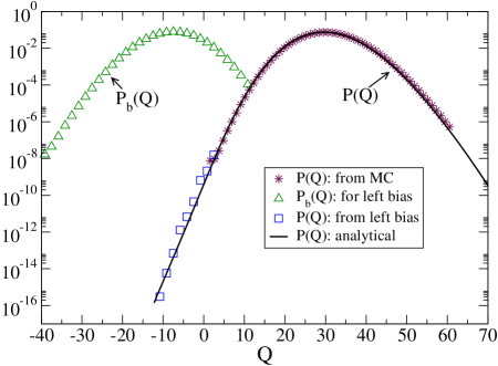
Thus $W$ and $Q$ are easily evaluated in the simulation using the biased dynamics. In Fig. (3) we show results for $P(Q,\tau)$ obtained both directly and using the biased dynamics. Again we see that for the same number of realizations ($10^{9}$) one can obtain probabilities about $10^{8}$ times smaller than using direct simulations. The comparison with the numerical results obtained from the exact expression for $\langle e^{-\lambda Q}\rangle$ visco06 also shows the accuracy of the algorithm.

Figure 4: (Color online) Plot of $P(Q)$ for $\tau=100$ for heat conduction across two particles connected by a harmonic spring with unit spring constant and $\gamma_{1}=\gamma_{2}=\sqrt{2},T_{1}=10,T_{2}=12$. MC refers to direct Monte Carlo simulations. The left bias corresponds to $\gamma_{1}^{\prime}=\gamma_{1},\gamma_{2}^{\prime}=\gamma_{2}/2,T_{1}^{\prime}=T_{1},T_{2}^{\prime}=2T_{2}$ and right bias to $\gamma_{1}^{\prime}=\gamma_{1}/2,\gamma_{2}^{\prime}=\gamma_{2},T_{1}^{\prime}=2T_{1},T_{2}^{\prime}=T_{2}$.

It is easy to apply the algorithm to more complicated cases. For example consider a one-dimensional chain of $L$ particles connected to heat reservoirs at the two ends with the following equations of motion:

$$m_{l}\dot{v}_{l} =f_{l}+\delta_{l,1}[-\gamma_{1}v_{1}+\sqrt{2D_{1}}\,\eta_{1}]$$

$$+\delta_{l,L}[-\gamma_{2}v_{L}+\sqrt{2D_{2}}\,\eta_{2}],~{}~{}~{}l=1,2,\dots,N~{},$$ (8)

where $f_{l}=-\partial_{x_{l}}U$ and $U(\{x_{l}\})$ is the potential energy of the system. The net heat transfer from the left bath into the system is given by $Q=\int_{0}^{\tau}(-\gamma_{1}v_{1}^{2}+\sqrt{2D_{1}}\eta_{1}v_{1})$ and using Eqs. (8) this can be expressed in terms of $\{x_{l},v_{l}\}$ as $Q=\int_{0}^{\tau}dtv_{1}(m_{1}\dot{v}_{1}-f_{1})$. To apply our algorithm we consider a biased dynamics where the Hamiltonian evolution is unchanged while the bath dynamics has new parameters $\gamma^{\prime}_{1},\gamma^{\prime}_{2},T^{\prime}_{1},T^{\prime}_{2}$ which are chosen so that $P_{b}(Q)$ has a peak in the required region. Choosing $D_{i}^{\prime}=D_{i}$ we again find $W$ by using Eqs. (8) in Eq. (7), as for the single particle case. Thus both $Q$ and $W$ can be expressed in terms of the path and so are readily evaluated for every realization of the biased dynamics.

As an example we study the case $L=2$ with $U=(x_{1}-x_{2})^{2}/2$ and with $m_{1}=m_{2}=1$. For the special parameters $\gamma_{1}=\gamma_{2}=\sqrt{2}$ we use the results in Ref. SD07 to obtain $\langle e^{-\lambda Q}\rangle\sim e^{\mu(\lambda)\tau}$ with $\mu(\lambda)=\sqrt{2}\bigl{\{}1-[1+{\beta_{1}^{-1}\beta_{2}^{-1}\lambda(\Delta\beta-\lambda)}]^{1/6}\bigr{\}}$ . This can be inverted to numerically compute $P(Q,\tau)$ at large $\tau$. In Fig. (4) we give the comparison between the analytical distribution and that obtained by the biasing method.

V Conclusion

In conclusion, we have presented an algorithm for computing the probabilities of rare events in various nonequilibrium processes. The algorithm is an application of importance sampling and consists in using a biased dynamics to generate the required rare events. This algorithm is straightforward to understand and also to implement. The error in the estimate of $P(Q,\tau)$ is $\approx\langle e^{-2W}\delta_{Q,Q_{\bf x}}\rangle_{b}^{1/2}/[MP_{b}(Q)]^{1/2}$. In the systems that we have studied we find that the error can be made small by choosing the biased dynamics carefully. We have applied the algorithm to two different models of particle and heat transport and shown that in both cases it gives excellent results. We note, however, that, in general, the fluctuations in $W$ grow with $\tau$ and with the system size, hence the errors are large and finding an appropriate biased dynamics is not always easy. Further work is necessary for improving the efficiency of the algorithm for general systems.