Mod/Resc Parsimony Inference

Abstract

We address in this paper a new computational biology problem that aims at understanding a mechanism that could potentially be used to genetically manipulate natural insect populations infected by inherited, intra-cellular parasitic bacteria. In this problem, that we denote by Mod/Resc Parsimony Inference, we are given a boolean matrix and the goal is to find two other boolean matrices with a minimum number of columns such that an appropriately defined operation on these matrices gives back the input. We show that this is formally equivalent to the Bipartite Biclique Edge Cover problem and derive some complexity results for our problem using this equivalence. We provide a new, fixed-parameter tractability approach for solving both that slightly improves upon a previously published algorithm for the Bipartite Biclique Edge Cover. Finally, we present experimental results where we applied some of our techniques to a real-life data set.
Keywords: Computational biology, biclique edge covering, bipartite graph, boolean matrix, NP-completeness, graph theory, fixed-parameter tractability, kernelization.

1 Introduction

Wolbachia is a genus of inherited, intra-cellular bacteria that infect many arthropod species, including a significant proportion of insects. The bacterium was first identified in 1924 by M. Hertig and S. B. Wolbach in Culex pipiens, a species of mosquito. Wolbachia spreads by altering the reproductive capabilities of its hosts [6]. One of these alterations consists in inducing so-called cytoplasmic incompatibility [7]. This phenomenon, in its simplest expression, results in the death of embryos produced in crosses between males carrying the infection and uninfected females. A more complex pattern is the death of embryos seen in crosses between males and females carrying different Wolbachia strains. The study of Wolbachia and cytoplasmic incompatibility is of interest due to the high incidence of such infections, amongst others in human disease vectors such as mosquitoes, where cytoplasmic incompatibility could potentially be used as a driver mechanism for the genetic manipulation of natural populations.

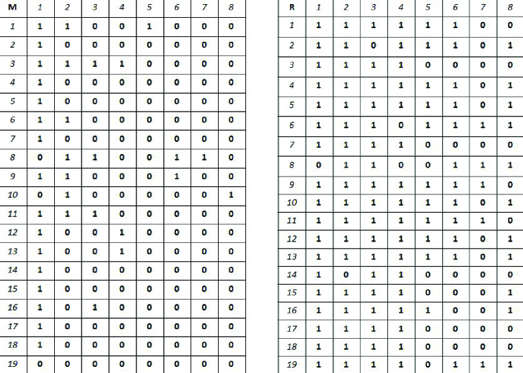
The molecular mechanisms underlying cytoplasmic incompatibility are currently unknown, but the observations are consistent with a “toxin / antitoxin” model [16]. According to this model, the bacteria present in males modify the sperm (the so-called modification, or mod factor) by depositing a “toxin” during its maturation. Bacteria present in females, on the other hand, deposit an antitoxin (rescue, or resc factor) in the eggs, so that offsprings of infected females can develop normally. The simple compatibility patterns seen in several insect hosts species [1, 2, 3] has lead to the general view that cytoplasmic incompatibility relies on a single pair of mod / resc genes. However, more complex patterns, such as those seen in Table 1 of the mosquito Culex pipiens [5], suggest that this conclusion cannot be generalized. The aim of this paper is to provide a first model and algorithm to determine the minimum number of mod and resc genes required to explain a compatibility dataset for a given insect host. Such an algorithm will have an important impact on the understanding of the genetic architecture of cytoplasmic incompatibility. Beyond Wolbachia, the method proposed here can be applied to any parasitic bacteria inducing cytoplasmic incompatibility.

Figure 1: The Culex pipiens dataset. Rows represent females and columns males.

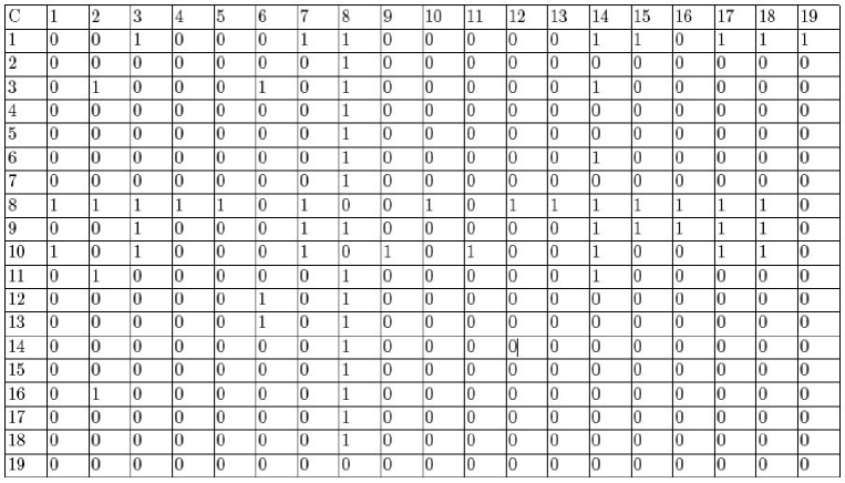
Let us now propose a formal description of this problem. Let the compatibility matrix $C$ be an $n$-by-$n$ matrix describing the observed cytoplasmic compatibility relationships among $n$ Wolbachia strains, with females in rows and males in columns. For the Culex pipiens dataset, the content of the $C$ matrix is directly given by Table 1. For each entry $C_{i,j}$ of this matrix, a value of $1$ indicates that the cross between the $i$’th female and $j$’th male is incompatible, while a value of $0$ indicates it is compatible. No intermediate levels of incompatibility are observed in Culex pipiens, so that such a discrete code (0 or 1) is sufficient to describe the data. Let the mod matrix $M$ be an $n$-by-$k$ matrix, with $n$ strains and $k$ mod genes. For each $M_{i,j}$ entry, a $0$ indicates that strain $i$ does not carry gene $j$, and a $1$ indicates that it does carry this gene. Similarly, the rescue matrix $R$ is an $n$-by-$k$ matrix, with $n$ strains and $k$ resc genes, where $R_{i,j}$ entries indicate whether strain $i$ carries gene $j$. A cross between female $i$ and male $j$ is compatible only if strain $i$ carries at least all the rescue genes matching the mod genes present in strain $j$. Using this rule, one can assess whether an $(M,R)$ pair is a solution to the $C$ matrix, that is, to the observed data.

We can easily find non-parsimonious solutions to this problem, that is, large $M$ and $R$ matrices that are solutions to $C$, as will be proven in the next section. However, solutions may also exist with fewer mod and resc genes. We are interested in the minimum number of genes for which solutions to $C$ exist, and the set of solutions for this minimum number. This problem can be summarized as follows: Let $C$ (compatibility) be a boolean $n$-by-$n$ matrix. A pair of $n$-by-$k$ boolean matrices $M$ (mod) and $R$ (resc) is called a solution to $C$ if, for any row $j$ in $R$ and row $i$ in $M$, $C_{i,j}=0$ if and only if $R_{j,\ell}\geq M_{i,\ell}$ holds for all $\ell$, $1\leq\ell\leq k$. This appropriately models the fact stated above that, for any cross to be compatible, the female must carry at least all the rescue genes matching the mod genes present in the male. For a given matrix $C$, we are interested in the minimum value of $k$ for which solutions to $C$ exist, and the set of solutions for this minimum $k$. We refer to this problem as the Mod/Resc Parsimony Inference problem (see also Section 2). Since in come cases, data (on females or males) may be missing, the compatibility matrix $C$ has dimension $n$-by-$m$ for $n$ not necessarily equal to $m$. We will consider this more general situation in what follows.

In this paper, we present the Mod/Resc Parsimony Inference problem and prove it is equivalent to a well-studied graph-theoretic problem known in the literature by the name of Bipartite Biclique Edge Cover. In this problem, we are given a bipartite graph, and we want to cover its edges with a minimum number of complete bipartite subgraphs (bicliques). This problem is known to be NP-complete, and thus Mod/Resc Parsimony Inference turns out to be NP-complete as well. In Section 4, we investigate a previous fixed-parameter tractability approach [8] for solving the Bipartite Biclique Edge Cover problem and improve its algorithm. In addition, we show a reduction between this problem and the Clique Edge Cover problem. Finally, in Section 5, we present experimental results where we applied some of these techniques to the Culex pipiens data set presented in Table 1. This provided a surprising finding from a biological point of view.

2 Problem Definition and Notation

In this section, we briefly review some notation and terminology that will be used throughout the paper. We also give a precise mathematical definition of the Mod/Resc Parsimony Inference problem we study. For this, we first need to define a basic operation between two boolean vectors:

Definition 1

The $\otimes$ vectors multiplication is an operation between two boolean vectors $U,V\in\{0,1\}^{k}$ such that :

$$U\otimes V:=\left\{\begin{array}[]{lll}1&:&\quad U[i]>V[i]\textrm{ for some }i\in\{1,\ldots,k\}\\ 0&:&\quad\textrm{otherwise}\end{array}\right.$$

In other words, the result of the $\otimes$ multiplication is $0$ if, for all corresponding locations, the value in the second vector is not less than in the first.

The reader should note that this operation is not symmetric. For example, if $U:=(0,1,1,0)$ and $V:=(1,1,1,0)$, then $U\otimes V=0$, while $V\otimes U=1$. We next generalize the $\otimes$ multiplication to boolean matrices. This follows easily from the observation that the boolean vectors $U,V\in\{0,1\}^{k}$ may be seen as matrices of dimension $1$-by-$k$. We thus use the same symbol $\otimes$ to denote the operation applied to matrices.

Definition 2

The $\otimes$ row-by-row matrix multiplication is a function $\{0,1\}^{n\times k}\times\{0,1\}^{m\times k}\to\{0,1\}^{n\times m}$ such that $C=M\otimes R$ iff $C_{i,j}=M_{i}\otimes R_{j}$ for all $i\in\{1,\ldots,n\}$ and $j\in\{1,\ldots m\}$. (Here $M_{i}$ and $R_{j}$ respectively denote the $i$’th and $j$’th row of $M$ and $R$.)

Definition 3

In the Mod/Resc Parsimony Inference problem, the input is a boolean matrix $C\in\{0,1\}^{n\times m}$, and the goal is to find two boolean matrices $M\in\{0,1\}^{n\times k}$ and $R\in\{0,1\}^{m\times k}$ such that $C_{i,j}=M\otimes R$ and with $k$ minimal.

We first need to prove there is always a correct solution to the Mod/Resc Inference Problem. Here we show that there is always a solution for as many mod and resc genes as the minimum between the number of male and female strains in the dataset.

Lemma 1

The Mod/Resc Parsimony Inference problem always has a solution.

Proof

A satisfying output for the Mod/Resc Parsimony Inference problem always exists for any possible $C$ of size $n$-by-$m$. For instance, let $M$ be of size $n$-by-$n$ and equal to the identity matrix, and let $R$ be of size $m$-by-$n$ and such that $R=\overline{C}^{T}$. This solution is correct since the only $1$-value in an arbitrary row $r_{i}$ of the matrix $M$ is at location $M_{ii}$. Thus, the only situation where $C_{ij}=1$ is when $R_{ji}=0$, which is the case by construction. ∎

We will be using some standard graph-theoretic terminology and notation. We use $G$, $G^{\prime}$, and so forth to denote graphs in general, where $V(G)$ denotes the vertex set of a graph $G$, and $E(G)$ its edge-set. By a subgraph of $G$, we mean a graph $G^{\prime}$ with $V(G^{\prime})\subseteq V(G)$ and $E(G^{\prime})\subseteq E(G)$. For a bipartite graph $G$, i.e. a graph whose vertex-set can be partitioned into two classes with no edges occurring between vertices of the same class, we use $V_{1}(G)$ and $V_{2}(G)$ to denote the two vertex classes of $G$. A complete bipartite graph (biclique) is a bipartite graph $G$ with $E(G):=\{\{u,v\}:u\in V_{1}(G),v\in V_{2}(G)\}$. We will sometimes use $B$, $B_{1}$, and so forth to denote bicliques.

3 Equivalence to Bipartite Biclique Edge Cover

In this section, we show that the Mod/Resc Parsimony Inference problem is equivalent to a classical and well-studied graph theoretical problem known in the literature as the Bipartite Graph Biclique Edge Cover problem. Using this equivalence, we first derive the complexity status of Mod/Resc Parsimony Inference, and later devise FPT algorithms for this problem. We begin with a formal definition of the Bipartite Graph Biclique Edge Cover problem.

Definition 4

In the Bipartite Biclique Edge Cover Problem problem, the input is a bipartite graph $G$, and the goal is to find the minimum number of biclique subgraphs $B_{1},\ldots,B_{k}$ of $G$ such that $E(G):=\bigcup_{\ell}E(B_{\ell})$.

Given a bipartite graph $G$ with $V_{1}(G):=\{u_{1},\ldots,u_{n}\}$ and $V_{2}(G):=\{u_{1},\ldots,u_{m}\}$, the bi-adjacency matrix of $G$ is a boolean matrix $A(G)\in\{0,1\}^{n\times m}$ defined by $A(G)_{i,j}:=1\iff\{u_{i},v_{j}\}\in E(G)$. In this way, every boolean matrix $C$ corresponds to a bipartite graph, and vice versa.

Theorem 3.1

Let $C$ be a boolean matrix of size $n\times m$. Then there are two matrices $M\in\{0,1\}^{n\times k}$ and $R\in\{0,1\}^{m\times k}$ with $C=M\otimes R$ iff the bipartite graph $G$ with $A(G):=C$ has a biclique edge cover with $k$ bicliques.

Proof

$(\Longleftarrow)$ Let $G$ be the bipartite graph with the bi-adjacency matrix $C$, and suppose $G$ has biclique edge cover $B_{1},B_{2},\ldots,B_{k}$. We construct two boolean matrices $M$ and $R$ as follows: Let $V_{1}(G):=\{u_{1},\ldots,u_{n}\}$ and $V_{2}(G):=\{v_{1},\ldots,v_{m}\}$. We define:

1. $M_{i,\ell}=1\iff u_{i}\in V_{1}(B_{\ell})$.

2. $R_{j,\ell}=0\iff v_{j}\in V_{2}(B_{\ell})$.

An illustration of this construction is given in Figure 2.

Figure 2: Reduction illustrated.

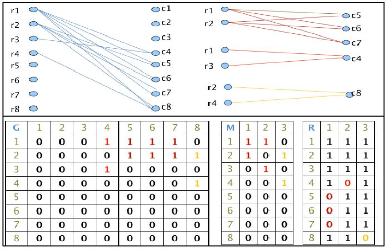
We argue that $C=M\otimes R$. Consider an arbitrary location $C_{i,j}=1$. By definition we have $\{u_{i},v_{j}\}\in E(G)$. Since the bicliques $B_{1},\ldots,B_{k}$ cover all edges of $G$, we know that there is some $\ell$, $\ell\in\{1,\ldots,k\}$, with $u_{i}\in V_{1}(B_{\ell})$ and $v_{j}\in V_{2}(B_{\ell})$. By construction we know that $M_{i,\ell}=1$ and $R_{j,\ell}=0$, and so $M_{i}\otimes R_{j}=1$, which means that the entry at row $i$ and column $j$ in $M\otimes C$ is equal to 1. On the other hand, if $C_{ij}=0$, then $\{u_{i},v_{j}\}\notin E(G)$, and thus there is no biclique $B_{\ell}$ with $u_{i}\in V_{1}(B_{\ell})$ and $v_{j}\in V_{2}(B_{\ell})$. As a result, for all $\ell\in\{1,\ldots,k\}$, if $M_{i,\ell}=1$ then $R_{i,\ell}=1$ as well, which means that the result of the $\otimes$ multiplication between the $i$’th row in $M$ and the $j$’th row in $R$ will be equal to 0.

$(\Longrightarrow)$ Assume there are two matrices $M\in\{0,1\}^{n\times k}$ and $R\in\{0,1\}^{m\times k}$ with $C=M\otimes R$. Construct $k$ subgraphs $B_{1},\ldots,B_{k}$ of $G$, where the $\ell$’th subgraph is defined as follows:

1. $u_{i}\in V_{1}(B_{\ell})\iff M_{i,\ell}=1$.

2. $v_{j}\in V_{2}(B_{\ell})\iff R_{j,\ell}=0$.

3. $\{u_{i},v_{j}\}\in E(B_{\ell})\iff\{v_{i},v_{j}\}\in E(G)$.

We first argue that each of the subgraphs $B_{1},\ldots,B_{k}$ is a biclique. Consider an arbitrary subgraph $B_{\ell}$, and an arbitrary pair of vertices $u_{i}\in V_{1}(B_{\ell})$ and $v_{j}V_{2}(B_{\ell})$. By construction, it follows that $M_{i,\ell}=1$ and $R_{i,\ell}=0$. As a result, it must be that $C_{i,j}=1$, which means that $\{u_{i},v_{j}\}\in E(G)$. Next, we argue that $\bigcup_{\ell}E(B_{\ell})=E(G)$. Consider an arbitrary edge $\{u_{i},v_{j}\}\in E(G)$. Since $C=A(G)$, we have $C_{i,j}=1$. Furthermore, since $M\otimes R=C$, there must be some $\ell\in\{1,\ldots,k\}$ with $M_{i,\ell}>R_{j,\ell}$. However, this is exactly the condition for having $u_{i}$ and $v_{j}$ in the biclique subgraph $B_{\ell}$. It follows that indeed $\bigcup_{\ell}E(B_{\ell})=E(G)$, and thus the theorem is proved. ∎

Due to the equivalence between Mod/Resc Parsimony Inference and Bipartite Biclique Edge Cover, we can infer from known complexity results regarding Bipartite Biclique Edge Cover the complexity of our problem. First, since Bipartite Biclique Edge Cover is well-known to be NP-complete [15], it follows that Mod/Resc Parsimony Inference is NP-complete as well. Furthermore, Gruber and Holzer [11] recently showed that Bipartite Biclique Edge Cover problem cannot be approximated within a factor of $n^{1/3-\varepsilon}$ unless P = NP where $n$ is the total number of vertices. Since the reduction given in Theorem 3.1 is clearly an approximate preserving reduction, we can deduce the following:

Theorem 3.2

Mod/Resc Parsimony Inference is NP-complete, and furthermore, for all $\varepsilon>0$, the problem cannot be approximated within a factor of $(n+m)^{1/3-\varepsilon}$ unless P = NP.

4 Fixed-parameter tractability

In this section, we explore a parameterized complexity approach [4, 9, 14] for the Mod/Resc Parsimony Inference problem. Due to the equivalence shown in the previous section, we focus for convenience reasons on Bipartite Biclique Edge Cover. In parameterized complexity, problem instances are appended with an additional parameter, usually denoted by $k$, and the goal is to find an algorithm for the given problem which runs in time $f(k)\cdot n^{O(1)}$, where $f$ is an arbitrary computable function. In our context, our goal is to determine whether a given input bipartite graph $G$ with $n$ vertices has a biclique edge cover of size $k$ in time $f(k)\cdot n^{O(1)}$.

4.1 The kernelization

Fleischner et al. [8] studied the Bipartite Biclique Edge Cover problem in the context of parameterized complexity. The main result in their paper is to provide a kernel for the problem based on the techniques given by Gramm et al. [10] for the similar Clique Edge Cover problem. Kernelization is a central technique in parameterized complexity which is best described as a polynomial-time transformation that converts instances of arbitrary size to instances of a size bounded by the problem parameter (usually of the same problem), while mapping “yes”-instances to “yes”-instances, and “no”-instances to “no”-instances. More precisely, a kernelization algorithm $\mathcal{A}$ for a parameterized problem (language) $\Pi$ is a polynomial-time algorithm such that there exists some computable function $f$, such that, given an instance $(I,k)$ of $\Pi$, $\mathcal{A}$ produces an instance $(I^{\prime},k^{\prime})$ of $\Pi$ with:

• $|I^{\prime}|+k^{\prime}\leq f(k)$, and

• $(I,k)\in\Pi\iff(I^{\prime},k^{\prime})\in\Pi$.

We refer the reader to e.g. [12, 14] for more information on kernelization.

A typical kernelization algorithm works with reduction rules, which transform a given instance to a slightly smaller equivalent instance in polynomial time. The typical argument used when working with reduction rules is that once none of these can be applied, the resultant instance has size bounded by a function of the parameter. For the Bipartite Biclique Edge Cover, two kernelization rules have been applied by Fleischner et al. [8]:

RULE 1: If $G$ has a vertex with no neighbors, remove this vertex without changing the parameter.

RULE 2: If $G$ has two vertices with identical neighbors, remove one of these vertices without changing the parameter.

Lemma 2 ([8])

Applying rules 1 and 2 of above exhaustively gives a kernelization algorithm for Bipartite Biclique Edge Cover that runs in $O(n^{3})$ time, and transforms an instance $(G,k)$ to an equivalent instance $(G^{\prime},k)$ with $|V(G^{\prime})|\leq 2^{k}$ and $|E(G^{\prime})|\leq 2^{2k}$.

We add two additional rules, which will be necessary for further interesting properties.

RULE 3: If there is a vertex $v$ with exactly one neighbor $u$ in $G$, then remove both $v$ and $u$, and decrease the parameter by one.

Lemma 3

Rule 3 is correct.

Proof

Assume a biclique cover of size $k$ of the graph, and assume that vertex $v$ is a member of some of the bicliques in this cover. By definition, at least one of the bicliques covers the edge $\{u,v\}$. Since this is the only edge adjacent to $v$, the bicliques that cover $\{u,v\}$ include only vertex $u$ among the vertices in its bipartite vertex class. If the bicliques do not cover all the edges of $u$, add them to each of the bicliques. ∎

RULE 4: If there is a vertex $v$ in $G$ which is adjacent to all vertices in the opposite bipartition class of $G$, then remove $v$ without decreasing the parameter.

Lemma 4

Rule 4 is correct.

Proof

After applying rule 3 above, each remaining vertex in the graph has at least two neighbors. Assume a biclique cover of size $k$ of all the edges except those adjacent to vertex $v$. Assume w.l.o.g. that $v\in V_{1}(G)$. Since each vertex $u\in V_{2}(G)$ has degree at least 2, it is adjacent to an edge which is covered by the biclique cover. It therefore belongs to some biclique in this cover. For each biclique in the cover, add now vertex $v$ to its set of vertices. Since $v$ is adjacent to all the vertices of $V_{2}(G)$, each changed component is a correct biclique and the new solution covers all the edges, including those of vertex $v$, and is of same size. ∎

Regarding the time complexity of the new rules we introduced, it is clear that once a vertex has been found in which a rule should be applied, applying each rule takes $O(n)$ time. Thus, including the time necessary to find such a vertex, the time required for each rule is $O(n)$. Since one can apply the reduction rules at most $O(n)$ time, the total time required for our extended kernelization remains $O(n^{3})$. We remark that although the new rules do not change the kernelization size, which remains $2^{k}$ vertices in a solution of size $k$, they will be useful in the following section.

4.2 Bipartite Biclique Edge Cover and Clique Edge Cover

In this section, we show the connection between the Bipartite Biclique Edge Cover and the Clique Edge Cover problems. We show that in the context of fixed-parameter tractability, we can easily translate our problem to the classical clique covering problem and then use it for a solution to our problem. For instance, it gives another way for the kernelization of the problem and can provide interesting heuristics, mentioned in [10].

Given a kernelized bipartite graph $G^{\prime}$ as an instance to the Bipartite Biclique Edge Cover problem, we transform $G^{\prime}$ into a (non-bipartite) graph $G^{\prime\prime}$ defined by $V(G^{\prime\prime}):=V(G^{\prime})$ and $E(G^{\prime\prime}):=E(G^{\prime})\cup\{\{u,v\}:u,v\in V_{1}(G^{\prime})\textrm{ or }u,v\in V_{2}(G^{\prime})\}$.

Theorem 4.1

The edges of $G^{\prime}$ can be covered with $k$ cliques iff the edges of $G^{\prime\prime}$ can be covered with $k+2$ cliques.

Proof

Suppose $B_{1},\ldots,B_{k}$ is a biclique edge cover of $G^{\prime}$. Then each $V(B_{i})$, $i\in\{1,\ldots,k\}$, induces a clique in $G^{\prime\prime}$. Furthermore, the only remaining edges which are not covered in $G^{\prime\prime}$ are the ones between vertices in $V_{1}(G^{\prime})$ and $V_{2}(G^{\prime})$, which can be covered by the two cliques induced by these vertex sets in $G^{\prime\prime}$. Altogether this gives us $k+2$ cliques that cover all edges in $G^{\prime\prime}$. Conversely, take a clique edge cover $K_{1},\ldots,K_{c}$ of $G^{\prime\prime}$. Due to the fourth kernelization rule, we know that there is no vertex in $V_{1}(G^{\prime})$ which is connected to all vertices in $V_{2}(G^{\prime})$, and vice-versa, in both $G^{\prime}$ and $G^{\prime\prime}$. It follows that there must be at least two cliques in $\{K_{1},\ldots,K_{c}\}$, say $K_{1}$ and $K_{2}$, with $V(K_{1})\subseteq V_{1}(G^{\prime})$ and $V(K_{2})\subseteq V_{2}(G^{\prime})$. Thus, there is a subset of the cliques in $\{K_{3},\ldots,K_{c}\}$ which have vertices in both partition classes of $G^{\prime}$, and which cover all the edges in $G^{\prime}$. Taking the corresponding bicliques in $G^{\prime}$, and adding duplicated bicliques if necessary, gives us $k$ bicliques that cover all edges in $G^{\prime}$. ∎

4.3 Algorithms

After the kernelization algorithm is applied, the next step is usually to solve the problem using brute-force. This is what is done in [8]. However, the time complexity given there is inaccurate, and the parametric-dependent time bound of their algorithm is $O(k^{4^{k}}2^{3k})=O(2^{2^{2k}\lg k+3k})$ instead of the $O(2^{2k^{2}+3k})$ bound stated in their paper. Furthermore, the algorithm they describe is initially given for the related Bipartite Biclique Edge Partition problem (where each edge is allowed to appear exactly once in a biclique), and the adaptation of such algorithm to the Bipartite Biclique Edge Cover problem is left vague and imprecise. Here, we suggest two possible brute-force procedures for the Bipartite Biclique Edge Cover problem, each of which outperforms the algorithm of [8] in the worst-case. We assume throughout that we are working with a kernelized instance obtained by applying the algorithm described in Section 4.1, i.e. a pair $(G^{\prime},k)$ where $G^{\prime}$ is a bipartite graph with at most $2^{k}$ vertices (and consequently at most $4^{k}$ edges).

The first brute-force algorithm:

For each $k^{\prime}\leq k$, try all possible partitions of the edge-set $E(G^{\prime})$ of $G^{\prime}$ into $k^{\prime}$ subsets. For each such partition $\Pi=\{E_{1},\ldots,E_{k^{\prime}}\}$, check whether each of the subgraphs $G^{\prime}[E_{1}],\ldots,G^{\prime}[E_{k^{\prime}}]$ is a biclique, where $G^{\prime}[E_{i}]$ is the subgraph of $G$ induced by $E_{i}$. If yes, report $G^{\prime}[E_{1}],\ldots,G^{\prime}[E_{k^{\prime}}]$ as a solution. If some $G^{\prime}[E_{i}]$ is not a biclique, check whether edges in $E(G^{\prime})\setminus E(G^{\prime}_{i})$ can be added to $E[G^{\prime}_{i}]$ in order to make the graph a biclique. Continue with the next partition if some graph in $G^{\prime}[E_{1}],\ldots,G^{\prime}[E_{k^{\prime}}]$ cannot be appended in this way in order to get a biclique, and otherwise report the solution found. Finally, if the above procedure fails for all partitions of $E(G^{\prime})$ into $k^{\prime}\leq k$ subsets, report that $G^{\prime}$ does not have a biclique edge cover of size $k$.

Lemma 5

The above algorithm correctly determines whether $G^{\prime}$ has a bipartite biclique edge cover of size $k$ in time $\frac{2^{2^{2k}\lg k+2k+\lg k}}{k!}$.

Proof

Correctness of the above algorithm is immediate in case a solution is found. To see that the algorithm is also correct when it reports that no solution can be found, observe that for any biclique edge cover $B_{1},\ldots,B_{k}$ of $G$, the set $\{E_{1},\ldots,E_{k}\}$ with $E_{i}:=E(G^{\prime}_{i})\setminus\bigcup_{j<i}E(G^{\prime}_{j})$ defines a partition of $E(G^{\prime})$ (with some of the $E_{i}$’s possibly empty), and given this partition, the algorithm above would find the biclique edge cover of $G^{\prime}$. Correctness of the algorithm thus follows.

Regarding the time complexity, the time needed for appending edges to each subgraph is at most $O(|(V(G^{\prime}))^{2}|)=O(2^{2k})$, and thus a total of $O(2^{2k}k)=O(2^{2k+\lg k})$ time is required for the entire partition. The number of possible partitions of $E(G^{\prime})$ into $k$ disjoint set is the Stirling number of the second kind $S(2^{2k},k)$, which has been shown in [13] to be asymptotically equal to $O(\frac{k^{4^{k}}}{k!}=\frac{2^{2^{2k}\lg k}}{k!})$. Thus, the total complexity of the algorithm is $\frac{2^{2^{2k}\lg k+2k+\lg k}}{k!}$. ∎

The second brute-force algorithm:

We generate the set $\mathcal{K}(G^{\prime})$ of all possible inclusion-wise maximal bicliques in $G^{\prime}$, and try all possible $k$-subsets of $\mathcal{K}(G^{\prime})$ to see whether one covers all edges in $G^{\prime}$. Correctness of the algorithm is immediate since one can always restrict oneself to using only inclusion-wise maximal bicliques in a biclique edge cover. To generate all maximal bicliques, we first transform $G^{\prime}$ into the graph $G^{\prime\prime}$ given in Theorem 4.1. Thus, every inclusion-wise maximal biclique in $G^{\prime}$ is an inclusion-wise maximal clique in $G^{\prime\prime}$. We then use the algorithm of [18] on the complement graph $\overline{G^{\prime\prime}}$ of $G^{\prime\prime}$, i.e. the graph defined by $V(\overline{G^{\prime\prime}}):=V(G^{\prime\prime})$ and $E(\overline{G^{\prime\prime}}):=\{\{u,v\}:u,v\in V(\overline{G^{\prime\prime}}),u\neq v,\textrm{ and }\{u,v\}\notin E(G^{\prime\prime})\}$.

Theorem 4.2

The Bipartite Biclique Edge Cover problem can be solved in $O(f(k)+n^{3})$ time, where $f(k):=2^{k2^{k-1}+3k}$.

Proof

Given a bipartite graph $G$ as an instance to Bipartite Biclique Edge Cover, we first apply the kernelization algorithm to obtain an equivalent graph $G^{\prime}$ with $2^{k}$ vertices, and then apply the brute-force algorithm described above to determine whether $G^{\prime}$ has a biclique edge cover of size $k$. Correctness of this algorithm follows directly from Section 4.1 and the correctness of the brute-force procedure. To analyze the time complexity of this algorithm, we first note that Prisner showed that any bipartite graph on $n$ vertices has at most $2^{n/2}$ inclusion-wise maximal bicliques [18]. This implies that $|\mathcal{K}(G^{\prime})|\leq 2^{2^{k-1}}$. The algorithm of [17] runs in $O(|V(G^{\prime})||E(G^{\prime})||\mathcal{K}(G^{\prime})|)$ time, which is $O(2^{k}2^{2k}2^{2^{k-1}})=O(2^{2^{k-1}+3k})$. Finally, the total number of $k$-subsets of $\mathcal{K}(G^{\prime})$ is $O(2^{k2^{k-1}})$, and checking whether each of these subsets covers the edges of $G^{\prime}$ requires $O(|V(G^{\prime})||E(G^{\prime})|)=O(2^{3k})$ time. Thus, the total time complexity of the entire algorithm is $O(2^{2^{k-1}+3k}+2^{k2^{k-1}+3k}+n^{3})=O(2^{k2^{k-1}+3k}+n^{3}).$ ∎

It is worthwhile mentioning that some particular bipartite graphs have a number of inclusion-wise maximal bicliques, which is polynomial in the number of their vertices. For these types of bipartite graphs, we could improve on the worst-case analysis given in the theorem above. For instance, a bipartite chordal graph $G$ has at most $|E(G)|$ inclusion-wise maximal bicliques [18]. A bipartite graph with $n$ vertices and no induced cocktail-party graph of order $\ell$ has at most $n^{2(\ell-1)}$ inclusion-wise maximal bicliques [17]. The cocktail party graph of order $\ell$ is the graph with nodes consisting of two rows of paired nodes in which all nodes but the paired ones are connected with a graph edge (for a full definition, see [17]). Observing that the algorithm in Section 4.1 preserves cordiality and does not introduce any new cocktail-party induced subgraphs, we obtain the following corollary:

Corollary 1

The Bipartite Biclique Edge Cover problem can be solved in $O(2^{2k^{2}+3k}+n^{3})$ time when restricted to chordal bipartite graphs, and in $O(2^{2k^{2}(\ell-1)+3k}+n^{3})$ time when restricted to bipartite graphs with no induced cocktail-party graphs of order $\ell$.

5 Experimental Results

We performed experiments of the parameterized algorithms on the Culex pipiens dataset, given in Table 1. We implemented the algorithms in the C++ programming language, with source code of approximately 2500 lines.

The main difficulty in practice is to find the minimal size $k$. Different approaches could be used. One would proceed by first checking if there is no solution of small sizes since this is easy to check using the $FPT$ approach, and then increasing the size until reaching a smallest size $k$ for which one solution exists. Another would proceed by using different fast and efficient heuristics to discover a solution of a given size $k^{\prime}$ that in general will be greater than the optimal size $k$ sought. Then applying dichotomy (the optimal solution is between 1 and $k^{\prime}-1$), the minimal size could be found using the $FPT$ approach for the middle value between 1 and $k^{\prime}-1$, and so on. The source code and the results can be viewed on the webpage http://lbbe.univ-lyon1.fr/-Nor-Igor-.html.

The result obtained on the Culex pipiens dataset indicates that $8$ pairs of mod/resc genes are required to explain the dataset. This appear to be in sharp contrast to more simple patterns seen in other host species [2, 3, 1] that had led to the general belief that cytoplasmic incompatibility can be explained with a single pair of mod / resc genes. In biological terms, this result means that contrary to earlier beliefs, the number of genetic determinants of cytoplasmic incompatibility present in a single Wolbachia strain can be large, consistent with the view that it might involve repeated genetic elements such as transposable elements or phages.

6 Appendix

Figure 3: The Culex pipiens solution.

References

- [1] S.R. Bordenstein and J.H. Werren. Bidirectional incompatibility among divergent wolbachia and incompatibility level differences among closely related wolbachia in nasonia. Heredity, Sep(99(3)):278–87, 2007.
- [2] H. Merçot and S. Charlat. Wolbachia infections in drosophila melanogaster and d. simulans: polymorphism and levels of cytoplasmic incompatibility. Genetica, 120(1-3):51–9, 2004 Mar.
- [3] S.L. Dobson, E.J. Marsland, and W. Rattanadechakul. Wolbachia-induced cytoplasmic incompatibility in single- and superinfected aedes albopictus (diptera: Culicidae). J Med Entomol., May(38(3):382–7, 2001.
- [4] R.G. Downey and M.R. Fellows. Parameterized Complexity. Springer-Verlag, 1999.
- [5] O. Duron, C. Bernard, S. Unal, A. Berthomieu, C. Berticat, and M. Weill. Tracking factors modulating cytoplasmic incompatibilities in the mosquito culex pipiens. Mol Ecol., Sep(15(10)):3061–3071, 2006.
- [6] J. Engelstadter and G.D.D. Hurst. The ecology and evolution of microbes that manipulate host reproduction. Annual Review of Ecology, Evolution and Systematics, (40):127–149, 2009.
- [7] J. Engelstadter and A. Telschow. Cytoplasmic incompatibility and host population structure. Heredity, (103):196–207, 2009.
- [8] H. Fleischner, E. Mujuni, D. Paulusma, and S. Szeider. Covering graphs with few complete bipartite subgraphs. Theoretical Computer Science, 410(21-23):2045–2053, 2009.
- [9] J. Flum and M. Grohe. Parameterized Complexity Theory. Springer, 2006.
- [10] J. Gramm, J. Guo, F. Huffner, and R. Niedermeier. Data reduction, exact, and heuristic algorithms for clique cover. In Proceedings of the 8th ACM/SIAM workshop on ALgorithm ENgineering and EXperiments (ALENEX), pages 86–94, 2006.
- [11] H. Gruber and M. Holzer. Inapproximability of nondeterministic state and transition complexity assuming PNP. In Proceedings of the 11th international conference on Developments in Language Theory (DLT), pages 205–216, 2007.
- [12] J. Guo and R. Niedermeier. Invitation to data reduction and problem kernelization. SIGACT News, 38(1):31–45, 2007.
- [13] A.D. Korshunov. Asymptotic behaviour of stirling numbers of the second kind. Diskret. Anal., 39(1):24–41, 1983.
- [14] R. Niedermeier. Invitation to Fixed-Parameter Algorithms. Oxford University Press, 2006.
- [15] J. Orlin. Contentment in graph theory: covering graphs with cliques. Indagationes Mathematicae, 80(5):406–424, 1977.
- [16] D. Poinsot, S. Charlat, and H. Merçot. On the mechanism of wolbachia-induced cytoplasmic incompatibility: confronting the models with the facts. Bioessays, 25(1):259–265, 2003.
- [17] E. Prisner. Bicliques in graphs I: Bounds on their number. Combinatorica, 20(1):109–117, 2000.
- [18] S. Tsukiyama, M. Ide, H. Ariyoshi, and I. Shirakawa. A new algorithm for generating all the maximal independent sets. SIAM Journal on Computing, 6(3):505–517, 1977.