Abstract

We consider the intensity surface of a 2D image, we study the evolution of the symmetry sets (and medial axes) of 1-parameter families of iso-intensity curves. This extends the investigation done on 1-parameter families of smooth plane curves (Bruce and Giblin, Giblin and Kimia, etc.) to the general case when the family of curves includes a singular member, as will happen if the curves are obtained by taking plane sections of a smooth surface, at the moment when the plane becomes tangent to the surface.
Key words and phrases: Isophote curve, symmetry set, medial axis, skeleton, vertex, inflexion, shape analysis.

1 Introduction

Image data is often thought of as a collection of pixel values $I:Z^{2}\mapsto Z_{+}$. The physical information is better captured by embedding the pixel values in the real plane, as the pixelation and quantization are artifacts of the camera, hence $I:{\bf R}^{2}\mapsto{\bf R}_{+}$. The geometrical information of an image is even better captured looking at the level sets $I(x)=I_{0}$, for all $I_{0}\in{\bf R}_{+}$, that is, looking at the isophote curves of the image.

Shape analysis using point-based representations or medial representations (such as skeletons) has been widely applied on an object level demanding object segmentation from the image data. We propose to combine the object representation using a skeleton or symmetry set representation and the appearance modelling by representing image information as a collection of medial representations for the level-sets of an image. As the level $I_{0}$ changes, the curves change like sections of a smooth surface by parallel planes.

The qualitive changes in the medial representation of families of isophotes fall into two types: (1) those for which the isophotes remain nonsingular (see for example [3, 11]) and (2) those for which one isophote at least is singular. The symmetry set (SS) of a plane curve is the closure of the set of centres of circles which are tangent to the curve at two or more different places. The medial axis (MA) is the subset of the SS consisting of the closure of the locus of centres of circles which are maximal, (maximal means that the minimum distance from the centre to the curve equals the radius). Our aim is to extend the investigation to the case (2) when the family includes singular curves, as is the case when one of the plane sections is tangent to the surface so that this section is a singular curve. The final goal is to represent image smooth surfaces by the collection of all medial reprentations of isophotes, forming a singular surface in scale space.

In this article, which is theoretical in nature, we work with the full SS, and consider the transitions which occur in the SS of a family of plane sections of a generic smooth surface in 3-space, as the plane moves through a position where it is tangent to the surface. We investigate the local geometry of these families of curves and track the evolution of some crucial features of the SS and MA. In particular, we will trace and classify the patterns of some special points, on the sections of a surface as the section passes through a tangential point, such as vertices (maxima and minima of curvature), inflexions, triples of points where a circle is tritangent and the pattern of the centre of such a circle, paires of points where a circle is bitangent with a higher order contact at one of them, etc. The vertices are crucial to the understanding of the SS since it has branches which end at the centres of curvature at vertices. From the way in which vertices behave we can deduce a good deal about the evolution of the SS and its local number of branches. The inflexions correspond to where the evolute of the curve, recedes to infinity. We also classify all possible scenarii of how vertices and inflexions are distributed along the level curves.

Last, we produce examples of SS and MA illustrating the cases.

We are concerned with the local behaviour of symmetry sets (SS) and medial axis (MA) of plane sections of generic smooth surfaces so we may assume that our surface $M$ is given by an equation $z=f(x,y)$ for a smooth function $f$, which will often be assumed to be a polynomial of sufficiently high degree. We shall take $M$ in Monge form, that is $f,f_{x}$ and $f_{y}$ all vanish at (0,0).

Figure 1: Two plane sections of a torus close to a singular section, together with their evolutes. The thick lines are the MA and the dashed lines are the additional parts of the SS. As the two ovals merge, two cusps on the evolute recede to infinity, taking the branches of the SS with them. (In the right-hand figure, in fact the SS goes twice to infinity and in between these excursions it covers the whole vertical line; this part, caused by the global structure of the curve, has been omitted for clarity. In this paper we are concerned with the local behaviour of SS near the singular section.)

Acknowledgements  This work is a part of the DSSCV project supported by the IST Programme of the European Union (IST-2001-35443). The authors are also grateful to Prof. Mads Nielsen and Dr. Aleksander Pukhlikov for useful discussions.

2 Intrinsic geometry of generic isophote curves

This section describes the geometry of isophote curves evolving on a fixed smooth surface $M$, under a 1-parameter family of parallel plane sections. Namely, we shall examine closely the different configurations of vertices and inflexions on the sections on our surface. We will in particular concentrate on the evolution through a plane section which is tangent to $M$ at a point p, so that this section is singular. For a generic surface, three situations arise, according to the contact between the tangent plane and $M$ at p, as measured by the singularity type of the height function in the normal direction at p. See for example [15] for the geometry of these situations, and [4, 14] for an extensive discussion of the singularity theory.
$\bullet$   The contact at p is ordinary (‘$A_{1}$ contact’), in which case the point is (i) elliptic or (ii) hyperbolic. The intersection of $M$ with its tangent plane at p is locally an isolated point or a pair of transverse arcs.
$\bullet$   The contact is of type $A_{2}$, which means that p is parabolic. The intersection of $M$ with its tangent plane at p is locally a cusped curve.
$\bullet$   The contact is of type $A_{3}$, which means that p is a cusp of Gauss, in which case it can be (i) an elliptic cusp, or (ii) a hyperbolic cusp. The intersection with the tangent plane is locally an isolated point or a pair of tangential arcs.
Elliptic and hyperbolic points occupy regions of $M$, separated by parabolic curves which are generically nonsingular; on the parabolic curves are isolated points which are cusps of Gauss.

The following gives a complete description of the behaviour of vertices and inflexions on isophotes curves near a singular point.

Theorem 1.

Let $f=k$ be a section of a generic surface M by a plane close to the tangent plane at p, $k=0$ corresponding with the tangent plane itself. Then for every sufficiently small open neighbourhood $U$ of p in M, there exists $\varepsilon>0$ such that $f=k$ has exactly $v({\bf p})$ vertices and $i({\bf p})$ inflexions lying in $U$, for every $0<|k|\leq\varepsilon$, where $v({\bf p})$ and $i({\bf p})$ satisfy the following equalities.

1. If p is an elliptic point, then for one sign of $k$ the section is locally empty; in the non-umbilic case, for the sign of $k$ yielding a locally nonempty intersection we have $v({\bf p})=4$, $I({\bf p})=0$. Likewise if p is an umbilic point, then $v({\bf p})=6$, $I({\bf p})=0$.

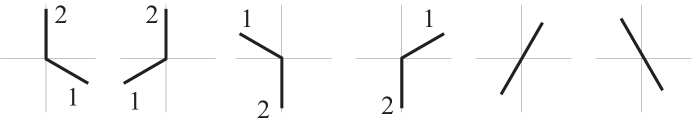
2. If p is a hyperbolic point, v(p) satisfies one of the following. We use $\leftrightarrow$ to indicate the transition in either direction, $m+n$ indicating the numbers of vertices on the two branches of $f=k$ for one sign of $k$ before the $\leftrightarrow$ and for the other sign of $k$ after it. In the most generic case (open regions of our surface) we have $2+2\leftrightarrow 2+2$ or $1+1\leftrightarrow 3+3$. See Figure 2. In other cases, occurring along curves or at isolated points of our surface, we can have in addition $3+2\leftrightarrow 2+1$ or $3+1\leftrightarrow 2+2$. Also using the same notation, $i({\bf p})$ satisfies: $1+1\leftrightarrow 0+2$ or $1+2\leftrightarrow 0+1$. There are 8 cases in all, and the full list is given in [9].

3. If p is a parabolic point but not a cusp of Gauss, $v({\bf p})=3$, $I({\bf p})=2$.

4. If p is an elliptic cusp of Gauss, $v({\bf p})=4$ , $I({\bf p})=2$ for one sign of $k$, and $v({\bf p})=I({\bf p})=0$ for the other.

5. If p is a hyperbolic cusp of Gauss, $v({\bf p})$ satisfies $1+3\leftrightarrow 4+4$ or $2+2\leftrightarrow 4+4$, whereas $I({\bf p})$ satisfies $2+2\leftrightarrow 0+2$, $1+1\leftrightarrow 0+0$ or $1+1\leftrightarrow 0+4$.

For the proof and more details see [8], [9].

Figure 2: Arrangements of vertices and inflexions on the level sets of $f$, in the most generic hyperbolic case (called ${\bf H}_{1}$ in [9]). See Theorem 1. In each case, we show, above, the vertex and inflexion curves—that is, the loci of vertices and inflexions on the level sets of $f$—and, below, a sketch of the level curves for $f<0$, $f>0$, showing the positions of these vertices and inflexions. Thick lines: $f=0$ or $f=k$; thin solid lines: vertex curves; dashed lines: inflexion curves. Open circles: minima of curvature; solid circles: maxima of curvature; squares: inflexions.

3 Symmetry sets (SS) and medial axes (MA) of isophote curves

The SS of a smooth simple closed curve in ${\mathbb{R}}^{2}$ is made of piecewise smooth curves (locus of $A_{1}^{2}$’s), triple crossings ($A_{1}^{3}$), cusps ($A_{1}A_{2}$), endpoints ($A_{3}$) and the points at ‘infinity’ (they correspond to bitangent lines to the curve). See Fig 3.

$\bullet$ $A_{1}^{2}$: The centres of bitangent circles with ordinary tangency at both points.

$\bullet$ $A_{1}^{3}$: The centres of tritangent circles with ordinary tangency at all points. They are the triple crossings on the symmetry set.

$\bullet$ $A_{1}A_{2}$: They are the centres of bitangent circles which are osculating circles at one point of the curve and have an ordinary tangency at the other point. They lie on the evolute and are cusps on the symmetry set.

$\bullet$ $A_{3}$: They are the centres of circles of curvature at extrema of curvature on the curve, the endpoints of the symmetry set and the cusps on the evolute.

$\bullet$ Bitangent lines: the circle now has its centre at infinity so the SS goes to infinity.

Figure 3: (a)-(e): Illustration of the circles whose centres contribute to the symmetry set. (a) is an $A_{1}^{2}$, (b) an $A_{1}A_{2}$, (c) an $A_{1}^{3}$, (d) an $A_{3}$ and (e) a centre at $\infty$ (bitangent line). In the last case the circle has become a straight line and the centre is at infinity. Right: a schematic drawing of a tritangent circle and a level set $f=k$ for an umbilic point at the origin O. As $k\to 0$ the points of tangency trace out three curves which we call the ‘$A_{1}^{3}$ curves’. Calculation of these curves is given in §3.1. Once these curves are known we can calculate the locus of centres of the tritangent circles.

At inflexions the evolute goes to infinity and the sign of curvature changes. Thus a positive maximum of curvature will be followed by a negative minimum, which in terms of the absolute value of curvature is again a maximum.

Our approach to the study of SS of families of curves which include a singular curve is to trace the $A_{3}$ points, the inflexions, the $A_{1}A_{2}$ points and the $A_{1}^{3}$ points on the curves as they approach the point at which the singularity develops. In this way we obtain significant information about the SS themselves. The patterns of vertices and inflexions have been studied in detail and for all the relevant cases in [8] and in [9], as recalled in Section 2. Subsection 3.1 and 3.2 are devoted to the study of the locus of $A_{1}^{3}$ and $A_{1}A_{2}$ points, respectively. In Subsection 3.3 we derive information on the changes on the SS of families of isophotes curves.

3.1 $A_{1}^{3}$ points

The $A_{1}^{3}$ points are the centres of circles which are tangent (ordinary tangency) to $f=k$ (for any choice of $f$, such as hyperbolic or umbilic) at three distinct points. They occur at triple crossings on the SS. Instead of looking directly for the centres of those tritangent circles, we rather first look for the points where those circles are tangent to the curve $f=k$ (see Fig. 3, right, for a schematic picture of the umbilic case). Thus we expect to have three curves, the ‘$A_{1}^{3}$ curves’, having the origin as their limit point, along which the three contact points move. First, we want to find the limiting directions of these curves, ie the lines they are tangent to as $k\to 0$. After finding the limiting directions, we can then determine enough of a series expansion (possibly a Puiseux series) to decide how the $A_{1}^{3}$ curves lie with respect to the vertex curves, etc. which we have determined before. We will give an example of such a parametrization below.

The equations which determine the $A_{1}^{3}$ curves are of course highly non-linear. They are in fact 8 equations in 9 unknowns, thereby determining an algebraic variety in ${\mathbb{R}}^{9}$ which, when projected onto suitable pairs of coordinates, gives each $A_{1}^{3}$ curve in turn. There are two important features of these equations:
$\bullet$ Naturally they are symmetric in that the contact points can be permuted;
$\bullet$ The equations inevitably admit solutions obtained by making two of the tangency points coincide (‘diagonal’ solutions). This causes the algebraic variety in ${\mathbb{R}}^{9}$ to have components of dimension greater than 1 which we want in some way to discard.

We now set up the equations. Any circle has the form $C(x,y)=0$ where

$$C=x^{2}+y^{2}+2ax+2by+c,$$

so that the centre is $(-a,-b)$ and the radius is $r$ where $r^{2}=a^{2}+b^{2}-c$. However we prefer the parametrization by $(a,b,c)$ rather than $(a,b,r)$ since it results in equations which are linear in the parameters.

Let this circle be tangent to $f=k$ at the three points ${\bf p}_{i}=(x_{i},y_{i})$, $i=1,2,3$. There are 8 equations $F_{j}=0,\ j=1,\ldots,8$ which connect the 9 unknowns $x_{i},y_{i},a,b,c$.

$F_{1}:=f(x_{1},y_{1})-f(x_{2},y_{2})$,
$F_{2}:=f(x_{1},y_{1})-f(x_{3},y_{3})$,
$F_{i+2}:=x_{i}^{2}+y_{i}^{2}+2ax_{i}+2by_{i}+c,\ \ i=1,2,3$,
$F_{i+5}:=a\frac{\partial f}{\partial y}(x_{i},y_{i})-b\frac{\partial f}{\partial x}(x_{i},y_{i})+x_{i}\frac{\partial f}{\partial y}(x_{i},y_{i})-y_{i}\frac{\partial f}{\partial x}(x_{i},y_{i}),\ \ i=1,2,3.$

The meaning of the 8 equations is as follows.

$eq_{1}$:	$F_{1}=0$	${\bf p}_{1}$ and ${\bf p}_{2}$ in the same level curve of $f$;
$eq_{2}:$	$F_{2}=0$	${\bf p}_{1}$ and ${\bf p}_{3}$ in the same level curve of $f$;
$eq_{i+2}:$	$F_{i+2}=0$	${\bf p}_{i}$ lies on the circle $C,\ \ i=1,2,3$;
$eq_{i+5}$:	$F_{i+5}=0$	$C$ and the level set of $f$ through ${\bf p}_{i}$ are tangent at ${\bf p}_{i}.$

First from the three equations $eq_{i},\ i=3,4,5$, we can get $a$, $b$ and $c$ as functions of $x_{i},y_{i}$. Of course this is merely finding the circle through three given points, which need to be non-collinear, and in particular distinct, for a unique solution. More details about this will appear elsewhere.

Remark In the umbilic case, we can always rotate the coordinates to make $b_{0}=b_{2}$ in the expression of $f(x,y)$, as shown in [10]. Thus, from now on we assume $b_{0}=b_{2}$ for an umbilic point. Once having assumed $b_{0}=b_{2}$, we now make the genericity assumption that $b_{1}\neq b_{3}$. We shall also look for solutions for these equations for which the limiting directions (limiting angles to the positive $x$-axis) are distinct. This relates to the point made earlier, that our equations inevitably admit ‘diagonal’ solutions which we want to suppress. Thus we are assuming here that the limiting directions of the three $A_{1}$ contact points of our tritangent circle are distinct as the oval $f(x,y)=k$ shrinks to a point with $k\to 0$.

Proposition 1.

Generically, there are no triple crossings, nor cusps on the local branches of the symmetry set of isophotes curves near a hyberbolic point.

The limiting directions of the $A_{1}^{3}$ curves at an umbilic, making the assumptions in the above Remark, are at angles $t_{1},t_{2},t_{3}$ equal, in some order, to $90^{\circ}$, $-30^{\circ}$, $-150^{\circ}$ to the positive $x$-axis, or the ‘opposites’ of these, namely $-90^{\circ}$, $150^{\circ}$, $30^{\circ}$. This suggests strongly that there are always two triples of $A_{1}^{3}$ contact points tending to the origin as $k\to 0$.

Proposition 1 implies, as confirmed by experimental evidence (see Fig. 6), that there are in fact two triple crossings ($A_{1}^{3}$) in the symmetry set in the umbilic case. The proof of the Proposition is an explicit computation of the tangent cone of the algebraic variety defined by the above equations $F_{i}=0,\ i=1\ldots 8$. The branches $(x_{i},y_{i})$ corresponding to $(t_{1},t_{2},t_{3})=(90^{\circ},-30^{\circ},-150^{\circ})$ have the form
$((-2b_{1}b_{0}-6b_{0}b_{3}+3c_{3}+c_{1})t^{2}/6(b_{3}-b_{1})+\ldots,t)$,
$(\frac{1}{2}\sqrt{3}t+\ldots,-\frac{1}{2}t+\ldots)$ and $(-\frac{1}{2}\sqrt{3}t+\ldots,-\frac{1}{2}t+\ldots)$

The actual locus of $A_{1}^{3}$ points (triple intersections) on the symmetry set close to an umbilic point where $b_{0}=b_{2}$ as above and $b_{1}\neq b_{3}$, is $(-a(t),-b(t))$ where

$a(t)=\frac{b_{0}}{2}t^{2}+\frac{1}{16}(7b_{0}b_{1}+9b_{0}b_{3}-3c_{1}-c_{3})t^{3}+$ h.o.t.

$b(t)=\frac{1}{8}(b_{1}+3b_{3})t^{2}+\frac{1}{16}(b_{1}^{2}+3b_{1}b_{3}+4b_{0}^{2}+5c_{4}-c_{2}-3c_{0})t^{3}+$ h.o.t.

Generically this curve has an ordinary cusp at the origin.

3.2 $A_{1}A_{2}$ points

The $A_{1}A_{2}$ points are the centres of bitangent circles which are osculating at one point and have an ordinary tangency at the other one; they produce cusps on the symmetry set. As in the case of $A_{1}^{3}$ points (§3.1), we look in the first instance for the points where those circles are tangent to the level sets of $f$.

We find these curves by taking the circle $C$ to have equation $x^{2}+y^{2}+ax+by+c=0$ as in §3.1. This time after elimination of $a,b,c$ we obtain 3 equations in 4 unknowns instead of 5 equations in 6 unknowns. Let the circle $C$ be tangent to the same level set $f=k$ at the two points ${\bf p}_{i}=(x_{i},y_{i}),\ i=1,2$. We proceed to write down the corresponding conditions, defining functions $F_{i}$ as follows.

$F_{1}:=f(x_{1},y_{1})-f(x_{2},y_{2})$,
$F_{2}:=2a(x_{1}-x_{2})+2b(y_{1}-y_{2})+x_{1}^{2}+y_{1}^{2}-x_{2}^{2}-y_{2}^{2}$,
$F_{3}:=af_{y}(x_{1},y_{1})-bf_{x}(x_{1},y_{1})+x_{1}f_{y}(x_{1},y_{1})-y_{1}f_{x}(x_{1},y_{1})$,
$F_{4}:=af_{y}(x_{2},y_{2})-bf_{x}(x_{2},y_{2})+x_{2}f_{y}(x_{2},y_{2})-y_{2}f_{x}(x_{2},y_{2})$,
$F_{5}:=(a+x_{2})(f_{xx}f_{y}^{2}-2f_{xy}f_{x}f_{y}+f_{yy}f_{x}^{2})-f_{x}(f_{x}^{2}+f_{y}^{2})$ (derivatives at $(x_{2},y_{2})$.

We have the corresponding equations and their interpretations:

$eq_{1}:$	$F_{1}=0$	${\bf p}_{1}$ and ${\bf p}_{2}$ are in the same level set of $f$;
$eq_{2}:$	$F_{2}=0$	a circle with centre $(-a,-b)$ passes through ${\bf p}_{1}$ and ${\bf p}_{2}$;
$eq_{3}:$	$F_{3}=0$	this circle is tangent to the level set of $f$ through ${\bf p}_{1}$;
$eq_{4}:$	$F_{4}=0$	this circle is tangent to the level set of $f$ through ${\bf p}_{2}$;
$eq_{5}:$	$F_{5}=0$	this circle is the circle of curvature of the level set through ${\bf p}_{2}$.

We solve $eq_{2},eq_{3}$ for $a$ and $b$ and substitute in $eq_{4}$ and $eq_{5}$. We summarize the results as follows. See Figure 4. We assume as before that the limiting angles at which the $A_{1}$ and $A_{2}$ points approach the origin are distinct.

Proposition 2.

Generically, there are no cusps on the local branches of the symmetry set of isophotes curves near a hyperbolic point. The limiting angles in the umbilic case must be one of the following.
$A_{1}:-30^{\circ},\ A_{2}:90^{\circ};$ or $A_{1}:150^{\circ},\ A_{2}:-90^{\circ};$
$A_{1}:-150^{\circ},\ A_{2}:90^{\circ};$ or $A_{1}:30^{\circ},\ A_{2}:-90^{\circ};$
$A_{1}:60^{\circ},\ A_{2}:-120^{\circ}$ or vice versa;
$A_{1}:-60^{\circ},\ A_{2}:120^{\circ}$ or vice versa.

Figure 4: The possible limiting directions of $A_{1}$ and $A_{2}$ contact points of $A_{1}A_{2}$ circles, in the umbilic case with axes rotated so that $b_{0}=b_{2}$, assuming the limiting directions are unequal. Those labelled 1 are only $A_{1}$ directions and similarly for $A_{2}$. The unlabelled directions can be either, with $A_{1}$ and $A_{2}$ at $180^{\circ}$ to one another.

This means that there are six cusps ($A_{1}A_{2}$) on the SS in this umbilic case. In that case, we expect each cusp (which requires an $A_{1}$ and an $A_{2}$ contact) to use one of the above six solutions, for a definite choice of $A_{1}$ and $A_{2}$ in the last two cases.

3.3 Symmetry Sets (SS) and Medial Axes (MA)

As suggested by Theorem 1, Propositions 2 and 2, the local structure of the SS and MA of individual isophote curves and its transitions are as follows:

$\bullet$ parabolic points: the local structure of SS is just $3$ separate branches correponding to the $3$ vertices separated by inflexions (Theorem 1), see Fig. 5.

$\bullet$ nonumbilic elliptic points: the SS is made of just $2$ transverse arcs, one joining two centres of curvature at maxima of curvature and the other one two minima of curvature. The SS will look like itself and disappear as the curve shrinks to a point.

Figure 5: To the left: A schematic picture of the patterns of the vertices (vertex set $V_{p}=0$: thin solid line) and inflexions (inflexion set $I_{p}=0$: dashed line) of the level curves $f=k$ evolving through a parabolic point, together with the zero level set $f=0$ (thick line). The vertex set has two cuspidal branches and one smooth branch. The inflexion set has one cuspidal branch which is always below all cupidal branches and one smooth branch. The zero level set $f_{p}=0$ has one cuspidal branch which is always between the two cuspidal vertex branches. The level set $f_{p}=k$ then evolves so that the number of vertices remains as 3 and the number of inflexions as 2 for both signs of $k$, with $k$ small. In the middle and to the right: Symmetry sets (thin lines) of curves (thick lines) which are sections of a surface close to the tangent plane at a parabolic point. One sees $3$ vertices sepated by two inflexions on both before and after the transition. At the transitional moment itself, the branches reach right to the curve, which then has an ordinary cusp. Figure produced with LSMP[16].

$\bullet$ hyperbolic point: the SS and MA are made of smooth branches, which do not connect together to form cusps or crossings. This implies in particular that generically, the SS (and MA) is just given by the geometry of vertices and inflexions as well as how they are distributed along the isophote curves, as described in Section 2. The branches of the SS will start at endpoints which are the centres of curvature of the isophote curves at vertices and they point towards the corresponding vertex if the isophote curve has a local minimum of curvature, and away from the vertex where the curve has a maximum of curvature.

$\bullet$ near umbilics: the SS have generically two triple crossings and six cusps. Hence generically, the SS has one structure, as in Fig. 6.

Figure 6: Symmetry set and pre-symmetry set of $f=k$, in the umbilic case $f(x,y)=x^{2}+y^{2}+x^{3}-xy^{2}+2y^{3}$ and $k=0.09$. The figure to the right is the same as the left hand side one, but the symmetry set has been enlarged so that the two $A_{1}^{3}$ points (triple crossings) and the six $A_{1}A_{2}$ (cusps) are more visible. One can also see the six endpoints of the symmetry set, corresponding to the six vertices on the curve. Varying $k$ then the SS will still look like itself and disappear as $k\to 0$. This figure illustrates the results of Proposition 1 and Proposition 2.

For the drawing of the SS and MA, we will need the pre-symmetry set (preSS) which is the subset of the cartesian product $I\times I$ of the parameter space $I$, defined by the pairs $(s,t)$ corresponding to points ${\text{\bf}p}=\gamma(s)$ and ${\text{\bf}q}=\gamma(t)$ which contribute to the SS. That is, there is a circle tangent to $\gamma$ at the points $\gamma(s)$ and $\gamma(t)$. See Fig. 6

4 Evolution of symmetry sets of isophote curves in $1$-parameter families of surfaces

As explained in Section 2, given a generic surface $M$, elliptic and hyperbolic points occupy regions of $M$, separated by parabolic curves with isolated points on them which are cusps of Gauss. We can then consider moving from a hyperbolic point to a parabolic point of $M$. We can also realise this by evolving the surface in a 1-parameter family, of the form $z=x^{2}-\alpha^{2}y+b_{0}x^{3}+b_{1}x^{2}y+b_{2}xy^{2}+b_{3}y^{3}+...$, where $\alpha\to 0$ and $b_{3}\neq 0$. It turns out that, generically, the only hyperbolic points which exist sufficiently near a parabolic point are the ones corresponding to vertex transition $1+1\leftrightarrow 3+3$ in Theorem 1. The Figure 7 shows how the vertices behave on a 2-parameter family of plane sections near the tangent plane at a hyperbolic point, evolving to a family of sections near a parabolic point.

Figure 7: Transition of the patterns of vertices (thick curve) and inflexions (fin curve) on a 2-parameter family of plane sections $f_{\alpha}=k$ near the tangent plane at a hyperbolic point, evolving to a family of sections $f_{0}=k$ near a parabolic point. $f(x,y)=x^{2}-\alpha^{2}y^{2}+x^{3}+2x^{2}y-xy^{2}+y^{3}$. (a) $\alpha=1$ (hyperbolic); the vertex set has $4$ branches and the inflexion $2$. (b) $\alpha=0.3$, the top part (above x-axis) of two vertex branches join together to form a loop which is shrinking to the origine as $\alpha\to 0$. The vertex branch tangent to $x=0$ stays smooth. The other vertex branch bend to become a cusp. (c) $\alpha=0.05$: the vanishing loop. (d) As $\alpha\to 0$, the inflexion set exchanges branches: the top part (above x-axis) join together to make a smooth branch, whereas the bottom part form a cusp below the cuspidal vertex branches. Compare Figures 2 and 5.

5 Conclusion

This paper represents a step towards understanding the evolution of SS and MA of families of isophote curves, or more generally of families of plane sections of s generic surface in 3-space. The evolution of the MA depends, in an essential way, upon the underlying evolution of the SS [13], which is why we have concentrated on the SS in this paper. An interesting follow up of this work, would be to combine into a more global represention of an image by the collection of those individual representations, as a singular surface in scale space, whose sections are the individual SS and MA.

References

- [1] T.F.Banchoff, T.Gaffney and C.McCrory, Cusps of Gauss Mappings, Pitman Research Notes in Mathematics, 55, 1982.
- [2] J.W. Bruce and P.J. Giblin, Curves and Singularities Cambridge University Press, 2nd ed. (1992).
- [3] J.W. Bruce and P.J. Giblin, ‘Growth, motion and one-parameter families of symmetry sets’, Proc. Royal Soc.Edinburgh 104A (1986), 179–204.
- [4] J.W. Bruce, P.J. Giblin and F. Tari, ‘Parabolic curves of evolving surfaces,’ Int. J. Computer Vision. 17 (1996), 291–306.
- [5] J.W.Bruce, P.J.Giblin and F.Tari, ‘Ridges, crests and sub-parabolic lines of evolving surfaces’, Int. J. Computer Vision, 18 (1996), 195–210.
- [6] J.W.Bruce, P.J.Giblin and F.Tari, ‘Families of surfaces: focal sets, ridges and umbilics’, Math. Proc. Camb. Phil. Soc 125 (1999), 243–268.
- [7] J. N. Damon, S. M. Pizer, K. Siddiqi, G. Szekely and S. W. Zucker, Multiscale Medial Loci and Their Properties. Int. J. Computer Vision, 55(2-3), 155-179, 2003.
- [8] A. Diatta and P.J. Giblin, Technical Reports 4, 11 and 23 of the project ”Deep Structure, Singularities, and Computer Vision”. IST Programme of the European Union (IST-2001-35443).
- [9] A. Diatta and P.J. Giblin, ’Vertices and inflexions of plane sections of surfaces in .’ Real and Complex Singularities. Trends in Mathematics (2006), 71-97. http://arxiv.org/abs/math/0502552.
- [10] A Diatta, P.J.Giblin, B.Guilfoyle and W.Klingenberg, ’Level sets of functions and symmetry sets of surface sections.’ Mathematics of Surfaces. Lecture Notes in Computer Science, 3604 (2005), 147-160. http://arxiv.org/abs/math/0504393
- [11] P.J.Giblin and B.B.Kimia, ‘On the local form and Transitions of Symmetry Sets, Medial Axes, and Shocks’, Int. J. Computer Vision 54 (2003), 143–157.
- [12] P.J. Giblin and B.B. Kimia, ‘On the Intrinsic Reconstruction of Shape from its Symmetries’, IEEE Trans. Pattern Analysis and Machine Intelligence, 25 (2003), 895–911.
- [13] P.J. Giblin, Symmetry sets and medial axes in two and three dimensions. The mathematics of surfaces, IX (Cambridge, 2000), 306-321, Springer, London, 2000.
- [14] P.L. Hallinan, G.G. Gordon, A.L. Yuille, P. Giblin and D. Mumford, Two and three dimensional patterns of the face, Natick, Massachusetts: A.K.Peters 1999.
- [15] J.J. Koenderink, Solid Shape, M.I.T. Press (1990)
-
[16]
R.J.Morris, Liverpool Surface Modelling
Package,
http://www.amsta.leeds.ac.uk/rjm/lsmp/ See also
R.J.Morris, ‘The use of computer graphics for solving problems in singularity theory’, in Visualization in Mathematics, H.-C.Hege & K.Polthier, Heidelburg: Springer-Verlag (1997), 173–187, and
http://www.scs.leeds.ac.uk/pfaf/lsmp/SingSurf.html