A Gibbs Sampling Based MAP Detection Algorithm for OFDM Over Rapidly Varying Mobile Radio Channels

Abstract

In orthogonal frequency-division multiplexing (OFDM) systems operating over rapidly time-varying channels, the orthogonality between subcarriers is destroyed leading to inter-carrier interference (ICI) and resulting in an irreducible error floor. In this paper, a new and low-complexity maximum a posteriori probability (MAP) detection algorithm is proposed for OFDM systems operating over rapidly time-varying multipath channels. The detection algorithm exploits the banded structure of the frequency-domain channel matrix whose bandwidth is a parameter to be adjusted according to the speed of the mobile terminal. Based on this assumption, the received signal vector is decomposed into reduced dimensional sub-observations in such a way that all components of the observation vector contributing to the symbol to be detected are included in the decomposed observation model. The data symbols are then detected by the MAP algorithm by means of a Markov chain Monte Carlo (MCMC) technique in an optimal and computationally efficient way. Computational complexity investigation as well as simulation results indicate that this algorithm has significant performance and complexity advantages over existing suboptimal detection and equalization algorithms proposed earlier in the literature.

Index Terms- OFDM, MAP detection, Monte carlo technique, Gibbs sampling. Intercarrier interference, fast time-varying channels.

I Introduction

Orthogonal frequency-division multiplexing (OFDM) has been shown to be an effective method to overcome inter-symbol interference (ISI) caused by frequency-selective fading with a simple transceiver structure, and is consequently used in several existing wireless local and metropolitan area standards such as the IEEE 802.11 and IEEE 802.16 families. IEEE 802.11 wireless LAN (WLAN) technology has become very popular for providing data services to Internet users although its overall design and feature set are not well suited for outdoor broadband wireless access (BWA) applications[1]. Therefore, IEEE 802.16 has been developed as a new standard for BWA applications [2]. Recently, the much-anticipated Worldwide Interoperability for Microwave Access (WiMAX) technology was introduced to promote the 802.16 standards while introducing features to enable mobile broadband services at vehicular speeds beyond 120 km/h.

OFDM eliminates ISI and simply uses a one-tap equalizer to compensate multiplicative channel distortion in quasi-static channels. However, in fading channels with very high mobility, the time variation of the channel over an OFDM symbol period results in a loss of subchannel orthogonality which leads to inter-carrier interference (ICI). A considerable amount of research on OFDM receivers for quasi-static fading has been conducted, but a major hindrance to such receivers is the lack of mobility support [3]. Since mobility support is widely considered to be one of the key features in wireless communication systems, and in this case ICI degrades the performance of OFDM systems, OFDM transmission over very rapidly time varying multipath fading channels has been considered recently in a number of recent works [4, 5, 6, 7, 8, 9, 10, 11, 12, 13, 14, 15].

The techniques proposed in these works range from linear equalizers, based on the zero-forcing (ZF) or the minimum mean-squared error (MMSE) criterion [4, 5, 6, 7, 8, 10, 9, 11, 12, 13], to nonlinear equalizers based on decision-feedback or ICI cancelation [10, 9, 11, 12, 13, 14]. Also near maximum-likelihood approaches have been proposed [16]. It has been shown that nonlinear equalizers based on ICI cancelation generally outperform linear approaches [12, 13, 10, 11]. However, linear equalizers still preserve their importance mainly because they are less complex.

In [12], performances of Matched Filter (MF), Least Squares (LS), Minimum Mean Square Error (MMSE) and MMSE with Successive Detection (SD) techniques with optimal ordering have been investigated. However, since the number of subcarriers is usually very large in high speed wide-band wireless standards, even the linear MMSE equalizer considered in [12] demands very high computational load.

The specific structure of the Doppler-induced ICI in OFDM systems operating over highly mobile channels presents a distinctive feature of limited support of the Doppler spread that can be exploited by the receiver. References [6, 7, 8, 10, 9] exploit the banded character of the frequency-domain channel matrix to reach a complexity that is only linear in the number of subcarriers. In a certain sense, the assumption of a banded frequency-domain channel matrix is a natural extension of the time-invariant channel case, in which the frequency-domain channel matrix is diagonal and hence banded with the smallest possible bandwidth.

In [7], using the banded structure of the channel matrix, a simple frequency domain equalizer has been proposed that can compensate for the loss of subchannel orthogonality due to ICI. However, the detection performance of the technique degrades substantially, since the data to be detected cannot fully use the contributing observation elements. The work presented in [13] combined [7] and [10] to derive a recursive decision feedback equalizer receiver for ICI suppression. The iterative MMSE serial linear equalizer (SLE) of [10], which takes the banded structure of the channel matrix into account, seems to be one of the most promising approaches to compensate for ICI. Iterative MMSE is then applied to estimate frequency-domain symbols. In [8], a block MMSE equalizer for OFDM systems operating over time-varying channels is presented. By exploiting the banded structure of the frequency-domain channel matrix, the complexity of the resulting algorithm turns out to be smaller than that of [10].

In this paper, a new computationally feasible, maximum a posteriori probability (MAP)-based data symbol detection algorithm is proposed for OFDM systems operating over highly mobile channels, as an alternative to the existing suboptimal equalization/detection techniques summarized in the above paragraphs. The proposed detection algorithm exploits the banded structure of the frequency-domain channel matrix whose bandwidth is a parameter to be adjusted according to the speed of the mobile terminal. This assumption enables us to decompose the main received signal vector into finite numbers of reduced-dimensional, sub-received signal vectors from which the data symbols can be detected by the MAP algorithm in an optimal and computationally efficient way. The decomposition is achieved in such a way that all the components of the received vector that contribute to the symbol to be detected are included in the decomposed observation model. Data symbols in each sub-received signal model are then detected successively by a MAP detection algorithm. To implement MAP symbol detection in a computationally efficient way, we employ a Markov Chain Monte Carlo (MCMC) technique based on Gibbs sampling, which is a powerful statistical signal processing tool to estimate a posteriori probability (APP) values.

The resulting detection algorithm is compared with previously proposed algorithms in terms of both bit error rate (BER) and complexity requirements. Computational complexity investigation as well as simulation results indicate that our algorithm has significant performance and complexity advantages over the existing suboptimal detection and equalization algorithms.

II System Model

Let us consider an OFDM system with $N$ subcarriers and available bandwidth $B=1/T_{s}$ where $T_{s}$ is the sampling period. A given sampling period is divided into $N$ subchannels by equal frequency spacing $\Delta f=B/N$. At the transmitter, information symbols are mapped into possibly complex-valued transmitted symbols according to the modulation format employed. The symbols are processed by an $N-$length Inverse Fast Fourier Transform (IFFT) block that transforms the data symbol sequence into the time domain. The time-domain signal is extended by a guard interval containing $G$ samples whose length is chosen to be longer than the expected delay spread to avoid ISI. The guard interval includes a cyclically extended part of the OFDM block to avoid ICI. Hence, the complete OFDM block duration is $P=N+G$ samples. The resulting signal is converted to an analog signal by a digital-to-analog (D/A) converter. After shaping with a low-pass filter (e.g. a raised-cosine filter) with bandwidth $B$, it is transmitted through the transmit antenna with the overall symbol duration of $PT_{s}$.

Let $h(m,l)$ represent the $l$th path (multipath component) of the time-varying channel impulse response at time instant $t=mT_{s}$. The discrete-time received signal can then be expressed as follows:

$$y(m)=\sum_{l=0}^{L-1}h(m,l)d(m-l)+w(m),$$ (1)

where the transmitted signal $d(m)$ at discrete sampling time $m$ is given by

$$d(m)=\frac{1}{\sqrt{N}}\sum_{k=0}^{N-1}s(k)e^{j2\pi mk/N},$$ (2)

$L$ is the total number of paths of the frequency selective fading channel, and $w(m)$ is additive white Gaussian noise (AWGN) with zero mean and variance $E\{|w(m)|^{2}\}=\sigma_{w}^{2}$. The sequence $s(k),k=0,1,\cdots,N-1,$ in (2) represent either quadrature-amplitude modulation (QAM) or phase-sift-keying (PSK) modulated data symbols with $E\{|s(k)|^{2}\}=1.$

At the receiver, after passing through the analog-to-digital (A/D) converter and removing the cyclic prefix (CP), a fast Fourier transform (FFT) is used to transform the data back into the frequency domain. Lastly, the binary data is obtained after demodulation and channel decoding.

The fading channel coefficients $h(m,l)$ can be modeled as zero-mean complex Gaussian random variables. Based on the wide-sense stationary uncorrelated scattering (WSSUS) assumption, the fading channel coefficients in different paths are uncorrelated with each other. However, these coefficients are correlated within each individual path and have a Jakes Doppler power spectral density having an autocorrelation function given by

$$E\{h(m,l)h^{*}(n,l)\}=\sigma^{2}_{h_{l}}J_{0}{(2\pi f_{d}T_{s}(m-n))},$$ (3)

where $\sigma^{2}_{h_{l}}$ denotes the power of the channel coefficients of the $l$th path. $f_{d}$ is the Doppler frequency in Hertz so that the term $f_{d}T_{s}$ represents the normalized Doppler frequency of the channel coefficients. $J_{0}(.)$ is the zeroth order Bessel function of the first kind.

By using (2) in (1), the received signal can be written as

$$y(m)=\frac{1}{\sqrt{N}}\sum_{k=0}^{N-1}s(k)\sum_{l=0}^{L-1}h(m,l)e^{j\frac{2\pi k(m-l)}{N}}+w(m),$$ (4)

which upon defining the time-varying channel transfer function

$$H(k,m)\triangleq{\sum}^{L-1}_{l=0}h(m,l)e^{-j2\pi lk/N},$$ (5)

becomes

$$y(m)=\frac{1}{\sqrt{N}}\sum_{k=0}^{N-1}s(k)H(k,m)e^{j2\pi mk/N}+w(m).$$ (6)

The FFT output at the $k^{th}$ subcarrier, after excluding the guard interval, can be expressed as

$$Y(k) = \frac{1}{\sqrt{N}}\sum_{m=0}^{N-1}y(m)e^{-j2\pi mk/N}$$ (7)

$$= s(k)G(k,k)+I(k)+W(k),$$

where $I(k)$ is ICI caused by the time-varying nature of the channel given as

$$I(k)=\sum_{i=0,i\neq k}^{N-1}s(i)G(k,i).$$ (8)

$G(k,i)$ in (8) represents the average frequency domain time-varying channel response, defined as

$$G(k,i)\triangleq(1/N)\sum_{m=0}^{N-1}H(i,m)e^{j2\pi m(i-k)/N}.$$ (9)

Similarly, the term $G(k,k)\triangleq\frac{1}{N}\sum_{m=0}^{N-1}H(k,m)$ in (9) represent the portion of the average frequency domain channel response at the $k$th subcarrier and $W(k)$ denotes discrete Fourier transform of the white Gaussian noise $w(m)$:

$$W(k)=\frac{1}{\sqrt{N}}\sum_{m=0}^{N-1}w(m)e^{-j2\pi mk/N}.$$ (10)

Because of the term $I(k)$ in (7), there is an irreducible error floor even in the training sequences since pilot symbols are also corrupted by ICI, arising from the fact that the time-varying channel destroys the orthogonality between subcarriers. Therefore, channel estimation should be performed either jointly with data or before the FFT block in order to compensate for the ICI. Note that if the channel is static or very slowly time-varying, that is $H(k,m)\thickapprox H(k)$, then it can be easily shown that $G(k,k)=H(k)$ and $I(k)=0$ for $k=0,1,\cdots,N-1,$ resulting in a received signal at the output of the FFT processor corresponding to the $k$th OFDM symbol given by

$$Y(k)=H(k)s(k)+W(k).$$

From (6) and (7), the FFT output received signal can be expressed in vector form as

$$\bf{Y}=\bf{G}\bf{s}+\bf{W}$$ (11)

where ${\bf{Y}}=[Y(0),Y(1),...,Y(N-1)]^{T}$, ${\bf{s}}=[s(0),s(1),...,s(N-1)]^{T}$ and ${\bf{W}}=[W(0),W(1),...,W(N-1)]^{T}.$ For $k,i=0,1,\cdots,N-1,$ the $(k,i)$th element of the matrix ${\bf G}=[G(k,i)]\in\mathcal{C}^{N\times N}$ representing the time-varying channel is given by (9).

Under the assumption that the channel matrix ${\bf G}$ in (11) is perfectly known at the receiver, the maximum likelihood (ML) detector performs an exhaustive search over the entire set of signal vectors whose components are selected from the signal constellation formed by the modulation scheme chosen. Especially in IEEE 802.16 based systems, the length $N$ of each OFDM symbol is very large; it can take values as large as $N=1024$ or even $N=2048$ especially for high mobility applications. In this case an exhaustive search for the ML solution would be very complex since the search space has an extremely large number of constellation points, ($|\mathcal{S}|^{N}$, where $|\mathcal{S}|$ is the cardinality of the signal constellation). On the other hand, all of the lower complexity linear detectors given in Table 1 are suboptimal since they do not take into account the correlation of the components of the transformed noise and yield noise enhancement. Recently, a nonlinear recursive detection technique using the decision-feedback principle, namely the MMSE-SD algorithm (VBLAST), has been proposed [12]. The performance of VBLAST depends critically on the order in which the data vector components are processed. To minimize error propagation effects and to improve the detection of unreliable components, more reliable data vector components should be detected first. Therefore, the algorithm depends on calculation of the post-detection signal-to-interference-plus-noise ratio (SINR) based upon MMSE detection as a measure of reliability, and so the calculation of SINR is compulsory at each iteration. Therefore this algorithm is computationally intensive as a number of pseudo inverse operations need to be performed. Moreover, its complexity grows exponentially with the total number of subcarriers.

TABLE I: Linear Detection Methods

Method	Solution
Matched Filter (MF)	$\bf{\hat{s}}=\mbox{Q}\{\bf{G^{\dagger}}\bf{Y}\}$
Zero Forcing (ZF)	$\bf{\hat{s}}=\mbox{Q}\{(\bf{G^{\dagger}}\bf{G})^{-1}\bf{G^{\dagger}}\bf{Y}\}$
MMSE	$\bf{\hat{s}}=\mbox{Q}\{(\bf{G^{\dagger}}\bf{G}+{\bf I}_{N}\sigma_{w}^{2})^{-1}\bf{G^{\dagger}}\bf{Y}\}$

where ${\bf I}_{N}$ is the $N$-by-$N$ identity matrix.

III MAP Detection Algorithm

The necessity of detecting large numbers of symbols in OFDM systems employed especially in highly mobile and wide-band wireless systems represents a significant computational burden as well as creating some convergence problems. However, as is known [9], time-varying channels produce a nearly-banded channel matrix ${\bf G}$ whose only main diagonal, $Q$ subdiagonals and $Q$ superdiagonals are nonzero. The bandwidth $2Q+1$, which is defined as the total number of non-zero diagonals in ${\bf G}$, is a parameter to be adjusted according to the mobility-rate of the channel. The significant coefficients of ${\bf G}$ thus are confined to the $2Q+1$ central diagonals. The parameter $Q\in\{0,1,\cdots N/2-1\}$ controls the target ICI response length; larger $Q$ corresponds to a longer ICI span and, thus, increased estimation complexity. In general, $Q$ should be chosen proportional to the width of the Doppler spectrum of the channel.

We now present an optimal low-complexity MAP detection algorithm to detect the data symbols ${\bf s}$ from ${\bf Y}$ taking into account the banded structure of the channel matrix ${\bf G}$. From the observation ${\bf Y}$ in (11), the receiver attempt to detect the OFDM output symbol ${\bf s}$, assuming that ${\bf G}$ is completely known by the receiver. The banded structure of the channel matrix ${\bf G}$ implies that the data symbol $s(k),k=0,1,\cdots,N-1,$ contributes to a maximum of $2Q+1$ observation elements as follows:

$${\bf Y}_{k}=[Y(j_{k}),Y(j_{k}+1),\cdots,Y(i_{k})]^{T},\mbox{ for}$$ (12)

$$j_{k}=\max\{0,k-Q\}\hskip 8.53581pt\mbox{and}\hskip 8.53581pti_{k}=\min\{N-1,k+Q\}.$$

Based on this observation, the received signal in (11) can be decomposed into $N$ reduced-dimensional sub-observations from which the data symbols can be detected in an optimal and computationally efficient way. For a given index $k=0,1,\cdots,N-1$ and $Q$, it can be easily shown from (11) and (12) that

$${\bf Y}_{k}={\bf G}_{k}{\bf s}_{k}+{\bf W}_{k}$$ (13)

where, ${\bf s}_{k}=\left[{\bf s}(j_{k})\right]$, ${\bf W}_{k}=\left[{\bf W}(j_{k})\right]$, ${\bf G}_{k}=\left[G(i_{k},j_{k})\right]$, for

$$I_{L_{k}}\triangleq\max\{0,k-Q\}\leq i_{k}\leq I_{U_{k}}\triangleq\min\{N-1,k+Q\}$$ (14)

and

$$J_{L_{k}}\triangleq\max\{0,k-2Q\}\leq j_{k}\leq J_{U_{k}}\triangleq\min\{N-1,k+2Q\}.$$ (15)

Note that due to the banded structure of ${\bf G}$, some elements of the matrices ${\bf G}_{k}$ are zero and $\mbox{dim}({\bf G}_{k})\leq(2Q+1)\times(2(2Q+1)-1)$. The ${\bf G}_{k}$’s reach their maximum dimension when $2Q+1\leq k\leq(N-(2Q+1))$.

For $k=0,1,\cdots,N-1,$ the MAP estimate of the data symbol $s(k)$ given ${\bf Y}_{k}$ is

$$\widehat{s}_{MAP}(k)\equiv\widehat{s}(k)=\arg\max_{s(k)\in\mathcal{S}}P(s(k)|{\bf Y}_{k}),$$ (16)

where $\mathcal{S}$ denotes the set of signal constellation points from which $s(k)$ takes values. Based on this approach, $s(k)$ can be detected sequentially for $k=0,1,\cdots,N-1$, incorporating the outcomes of the previous estimates in a decision-feedback mode as follows.

$\blacksquare$ For $k=0$, determine the estimate $\widehat{s}(0)$ from (16).

$\blacksquare$ For $k=k+1$ modify the observation vector ${\bf Y}_{k}$ by subtracting the terms coming from the contributions of the estimated data symbols $\widehat{s}(0),\widehat{s}(1),\cdots,\widehat{s}(k-1)$ as

$$\widetilde{{\bf Y}}_{k}\triangleq{\bf Y}_{k}-\sum_{l=J_{L_{k}}}^{k-1}{\bf g}^{(l)}_{k}\widehat{s}(l)$$ (17)

where ${\bf g}^{(l)}_{k}$ is the $l$th column of ${\bf G}_{k}$ and $J_{L_{k}}$ and $J_{U_{k}}$ are defined in (15).

$\blacksquare$ Determine the MAP estimate of $\widehat{s}(k)$ from

$$\widetilde{{\bf Y}}_{k}=\widetilde{{\bf G}}_{k}\widetilde{{\bf s}}_{k}+{\bf W}_{k}$$ (18)

as

$$\widehat{s}(k)=\arg\max_{\widetilde{s}(k)\in\mathcal{S}}P(\widetilde{s}(k)|\widetilde{{\bf Y}}_{k}),$$ (19)

where

$$\widetilde{{\bf G}}_{k}\triangleq{\bf G}_{k}-\left[{\bf g}^{(0)}_{k},{\bf g}^{(1)}_{k},\cdots,{\bf g}^{(k-1)}_{k}\right],$$ (20)

and $\widetilde{{\bf s}}_{k}$ is the vector obtained by removing the first $k-1$ elements of ${\bf s}_{k}.$
$\blacksquare$ END IF $k=N-1$.

The major problem is finding the values of $\hat{s}_{MAP}(k)$ in a computationally efficient manner. To see this difficulty we assume that the data symbols are independent and identically distributed binary phase shift keying (BPSK), taking values of $+1$ and $-1$. Note that higher dimensional signal constellations can be treated similarly with a straightforward extension. The conditional probability of $\widetilde{s}(k)$ given the observation vector $\bf\widetilde{Y}_{k}$ can be expressed as

$$P(\widetilde{s}(k)=+1|\widetilde{{\bf Y}}_{k}) = \sum_{\widetilde{{\bf s}}_{\overline{k}}}P(\widetilde{s}(k)=+1,\widetilde{{\bf s}}_{\overline{k}}|\widetilde{{\bf Y}}_{k})$$ (21)

$$= \sum_{\widetilde{{\bf s}}_{\overline{k}}}P(\widetilde{s}(k)=+1|\widetilde{{\bf s}}_{\overline{k}},\widetilde{{\bf Y}}_{k})P(\widetilde{{\bf s}}_{\overline{k}}|\widetilde{{\bf Y}}_{k})$$

where the second identity follows by applying the chain rule of probability. The vector $\bf\widetilde{s}_{\overline{k}}$ in (21) is obtained by canceling the component $\widetilde{s}(k)$ in $\bf\widetilde{s}_{k}$ and the summation is over all possible values of $\bf\widetilde{s}_{\overline{k}}$. The number of combinations that $\bf\widetilde{s}_{\overline{k}}$ takes grows exponentially with the dimension of $\bf\widetilde{s}_{k}$ and thus becomes prohibitive for large values of the size of this vector. Thus, we resort to the Gibbs sampler, a Monte Carlo method to calculate the a posteriori probabilities of the unknown symbols.

III-A MAP Detection Based on Gibbs Sampling

The Gibbs sampler is an MCMC sampling method for numerical evaluation of multidimensional integrals. Its popularity is gained from the facts that it is capable of carrying out many complex Bayesian computations. In this section we briefly explain the application of the Gibbs sampling technique to our symbol detection problem where the observation process is given by (18). For notational convenience we drop the index $k$ and the ”tilde” from all the involved variables, e.g. ${\bf Y},{\bf G}$ are shorthand notations for $\widetilde{{\bf Y}}_{k},\widetilde{{\bf G}}_{k}$, respectively. (21) can then be expressed as

$$P(s(k)=+1|{\bf Y}) = \sum_{{\bf s}_{\overline{k}}}P(s(k)=+1|{\bf s}_{\overline{k}},{\bf Y})P({\bf s}_{\overline{k}}|{\bf Y})$$ (22)

$$= E_{{\bf s}_{\overline{k}}|{\bf Y}}\left\{P(s(k)=+1|{\bf s}_{\overline{k}},{\bf Y})\right\}.$$

According to the Gibbs sampling based statistical Monte Carlo estimation technique, an estimate of (22) can be evaluated by taking the empirical average

$$P(s(k)=+1|{\bf Y})=\frac{1}{N_{s}}\sum_{n=1}^{N_{s}}P(s(k)=+1|{\bf s}^{(n)}_{\overline{k}},{\bf Y})$$ (23)

where ${\bf s}^{(n)}_{\overline{k}}$ for $n=1,2,\cdots,N_{s}$ are samples drawn from the conditional distribution $P({\bf s}_{\overline{k}}|{\bf Y})$. There is a substantial body of literature concerning the Monte Carlo Gibbs sampling technique; see, e.g., [17],[18]. One possible version of the Gibbs sampler suitable for calculating the a posteriori probabilities in (21) may be summarized as follows.

Let ${\bf s}=[s(0),s(1),\cdots,s(N-1)]^{T}$ be a vector of unknown data symbols. Let ${\bf Y}$ be the observed signal. To generate random samples from the distribution $P({\bf s}|{\bf Y})$, given the samples from the $(n-1)$th iteration ${\bf s}^{(n-1)}=[s^{(n-1)}(0),s^{(n-1)}(1),\cdots,s^{(n-1)}(N-1)]^{T}$, the Gibbs algorithm iterates at the $n$th iteration as follows to generate the samples ${\bf s}^{(n)}=[s^{(n)}(0),s^{(n)}(1),\cdots,s^{(n)}(N-1)]^{T}$:
$\blacksquare$ Initialize ${\bf s}^{(0)}$ randomly;
$\blacksquare$ for $n=1,2,\cdots,N_{T}$ and for $k=0,1\cdots,N-1,$
draw sample $s^{(n)}_{k}$ from $P\left(s(k)|s^{(n)}_{0},\cdots,s^{(n)}_{k-1},s^{(n-1)}_{k+1},\cdots,s^{(n)}_{N-1}\right).$

Note that to ensure convergence, the Gibbs iteration is usually carried out for $N_{T}=N_{b}+N_{s}$ iterations. The first $N_{b}$ iterations of the loop is called the burn-in period which is necessary for the Monte Carlo simulation to reach its stationary distribution. Only the samples ${\bf s}^{(n)}=[s^{(n)}_{0},s^{(n)}_{1},\cdots,s^{(n)}_{N-1}]^{T},n=N_{b}+1,\cdots,N_{T}$, from the last $N_{s}$ iterations are used to calculate the expectation.

It is known that under regularity conditions [19, 18],

(i) the distribution of ${\bf s}^{(n)}$ converges to $P({\bf s}|{\bf y})$, as $n\rightarrow\infty$.
(ii) $(1/N_{s}\sum_{n=1}^{N_{s}}P(s(k)=+1|{\bf s}^{(n)}_{\overline{k}},{\bf Y})=\sum_{{\bf s}_{\overline{k}}}P(s(k)=+1|{\bf s}_{\overline{k}},{\bf Y})P({\bf s}_{\overline{k}}|{\bf Y})$, as $n\rightarrow\infty$.

III-B Implementation of the Symbol Detector

From the previous section, we recall that to compute $P(s(k)=+1|{\bf Y}_{k})=\sum_{{\bf s}_{\overline{k}}}P(s(k)=+1,{\bf s}_{\overline{k}}|{\bf Y}_{k})$, we need to perform the summation on the right-hand side of (22). When ${\bf s}$ has a large dimension, the exact evaluation of this summation may not be feasible and other more efficient techniques must be adopted. In this section the Gibbs sampling-based Monte Carlo method summarized in the previous section will be applied to develop a computationally efficient algorithm for calculation of the a posteriori probabilities $P(s(k)|{\bf Y}).$ From (23), it follows that we need to evaluate $P(s(k)=+1|{\bf s}^{(n)}_{\overline{k}},{\bf Y}),$ for $n=1,2,\cdots,N_{T}$. For this we define

$$\lambda^{(n)}_{k}\triangleq\ln\frac{P(s(k)=+1|{\bf s}^{(n)}_{\overline{k}},{\bf Y})}{P(s(k)=-1|{\bf s}^{(n)}_{\overline{k}},{\bf Y})},$$ (24)

from which it can be easily seen that

$$P(s(k)=+1|{\bf s}^{(n)}_{\overline{k}},{\bf Y})=\frac{1}{1+\exp\left(-\lambda^{(n)}_{k}\right)}.$$ (25)

$\lambda^{(n)}_{k}$ can be computed by expanding $P(s(k)=+1|{\bf s}^{(n)}_{\overline{k}},{\bf Y})$ as

$$P\left(s(k)=+1|{\bf s}^{(n)}_{\overline{k}},{\bf Y}\right)=$$ (26)

$$\frac{p\left({\bf Y}|s(k)=+1,{\bf s}^{(n)}_{\overline{k}})P(s(k)=+1,{\bf s}^{(n)}_{\overline{k}}\right)}{\sum_{s(k)\in\{+1,-1\}}p\left({\bf Y}|s(k)=+1,{\bf s}^{(n)}_{\overline{k}}\right)P\left(s(k)=+1,{\bf s}^{(n)}_{\overline{k}}\right)}.$$

The data symbols are assumed to be independent and equally likely, Therefore, it follows from (26) and (24) that

$$\lambda^{(n)}_{k}\triangleq\ln\frac{p({\bf Y}|s(k)=+1,{\bf s}^{(n)}_{\overline{k}})}{p({\bf Y}|s(k)=-1,{\bf s}^{(n)}_{\overline{k}})}.$$ (27)

Since $p({\bf Y}|{\bf s})\thicksim\exp(-|{\bf y}-{\bf G}{\bf s}|^{2})$, after some algebra, (27) can be expressed as

$$\lambda^{n}(s_{k})=\frac{1}{\sigma^{2}_{w}}\Re\left\{{\bf g}^{{\dagger}}_{k}({\bf Y}-{\bf G}_{\overline{k}}\mbox{ }{\bf s}_{\overline{k}})\right\},$$ (28)

where $(\cdot)^{{\dagger}}$ denotes the conjugate transpose and $\Re\{\cdot\}$ denotes the real part of its argument. ${\bf G}_{\overline{k}}$ is ${\bf G}$ with its $k$th column $\bf{g}_{k}$ removed. In summary, for $k=0,1,\cdots,N-1$, to estimate the a posteriori probabilities $P(s(k)|{\bf Y})$ in (21), the Gibbs sampler runs over all symbols $N_{s}$ times to generate a collection of vectors $\left\{{\bf s}^{(n)}_{\overline{k}}\right\}_{n=N_{b}+1}^{N_{T}}$ which are used in (23) to compute the desired quantities.

III-C Complexity Requirements

The computational complexity of the MAP symbol detector based on Gibbs sampling proposed in this work is determined by the parameters $N_{s},Q,N$ and the constellation size of the transmitted data symbols. The computation of $\widetilde{{\bf Y}}_{k}$ in (18) for $k=0,1,\cdots,N-1$ requires a maximum of $(4Q^{2}+2Q)N$ complex multiplications (CMs) and $(4Q^{2}+2Q)N$ complex additions (CAs) per data block. Assuming BPSK signaling, the computation of the a posteriori probabilities in (22) requires a maximum of $(8Q^{2}+2Q+1)NN_{s}$ CMs and $(8Q^{2}+2Q-1)NN_{s}$ CAs and computation of the empirical average of a posteriori probabilities of the data symbols in (23) requires $NN_{s}$ CSs. Therefore, the whole algorithm requires of maximum $N(4Q^{2}+2Q+(4Q^{2}+2Q)N_{s})$ CMs and $N(4Q^{2}+2Q+(4Q^{2}+2Q)N_{s})$ CAs, leading to a total of $2N(4Q^{2}+2Q+(4Q^{2}+2Q)N_{s})$ complex operations.

Several low complexity equalization algorithms have been developed recently, of which several are worth mentioning here to compare their computational complexities with that of the Gibbs-based algorithm.

Ruguni et al. [8] proposed a block MMSE technique based on exploiting the banded structure of the channel matrix ${\bf G}$. The matrix inversion was obtained using a low-complexity decomposition such as Cholesky or the $LDL^{{\dagger}}$ decomposition. The algorithm requires a total of $(8Q^{2}+22Q+4)N$ complex operations. Schniter [10] proposed a linear serial equalizer also based on exploiting the banded structure of the channel matrix. This algorithm requires a total of $(8/3Q^{3}+2Q^{2}+5/3Q+4)N$ complex operations. The complexity of the serial MMSE equalizer is higher than that of the block MMSE equalizer.

In the VBLAST algorithm, matrix inversion is needed of dimension equal to the number of OFDM subcarriers. As a result, the computational complexity of the VBLAST receiver increases rapidly with the number of subcarriers, which makes its real-time implementation prohibitive for large numbers of subcarriers.

As can be seen easily, the complexity of our algorithm is of the same order of the above equalization algorithms and is lower than the VBLAST algorithm. However, as remarked earlier, these algorithms are suboptimal as opposed to our optimal MAP detection algorithm and perform poorly especially when the ICI is high. It is also worth mentioning that our algorithm can be easily extended to an iterative multiuser MAP detection scheme for OFDM systems.

IV Simulation Results

This section presents computer simulation results of the proposed detection methods for rapidly varying mobile radio channels. The system operates with a 5 MHz bandwidth and is divided into 512 tones ($N=512$) with a total symbol period ($T_{s}$) of 115 $\mu$s, of which 12.8 $\mu$s constitute the CP. One OFDM symbol thus consists of 576 samples, sixty-four of which constitute the CP. The normalized Doppler frequencies are $f_{d1}*T_{s}=0.0307$ and $f_{d2}*T_{s}=0.1075$, corresponding to an IEEE 802.16e mobile terminal moving with speeds of 120 km/h and 420 km/h, respectively, for a carrier frequency of 2.4 GHz. The wireless channels between the mobile antenna and the receiver antenna are modeled based on a realistic channel model determined by the COST-207 project in which Typical Urban (TU) and Bad Urban (BU) channel models are considered. For each OFDM symbol, Gibbs sampling is performed for 30 iterations, with the first 10 iterations as the burn-in period.

Figure 1: BER comparison of various detection algorithms for OFDM systems; TU Channel (6 taps), 420 km/h

Figure 2: BER comparison of various detection algorithms for OFDM systems; TU Channel (6 taps), 120 km/h

Figure 3: BER comparison of various detection algorithms for OFDM systems; BU Channel (6 taps), 420 km/h

Figure 4: BER performance of the proposed MAP algorithm based on Gibbs Sampling for the TU channel as a function of Q values

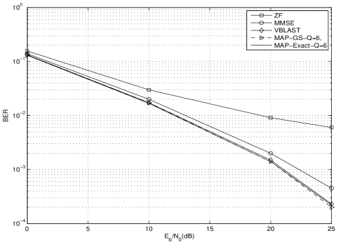
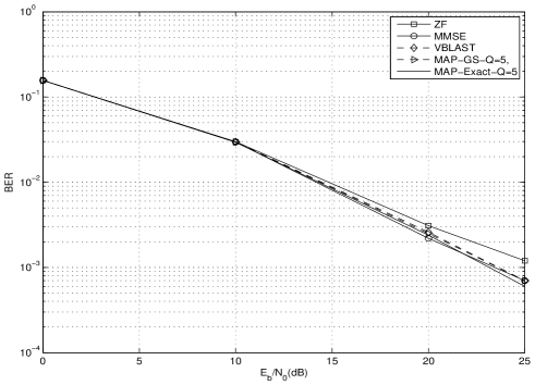
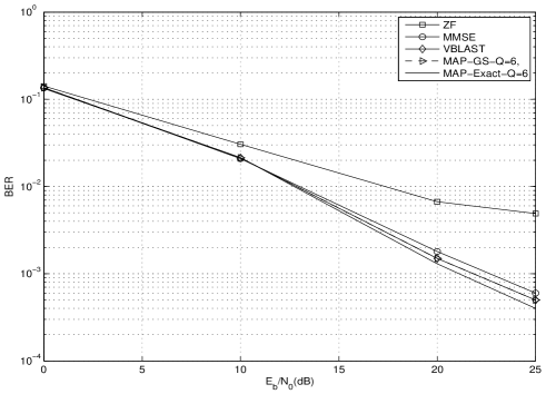
The information symbols are BPSK modulated to yield $\mathcal{S}$ = $\{\pm 1\}$. Figs.1-3 compare the BER performance of the proposed Gibbs-based MAP detection algorithm, an equalization technique based on zero forcing (ZF) proposed in [7], linear MMSE, and the VBLAST algorithm proposed in [12], as a function of energy per bit to noise power ratio ($E_{b}/N_{0}$) where $N_{0}$ is equal to $\sigma_{w}^{2}$.

ZF causes noise enhancement while it eliminates the ICI. Therefore, it is seen that ZF performance is the worst. The reason for this can also be explained by the ill-conditioned matrix $({\bf G}^{{\dagger}}{\bf G})$ to be inverted. This problem can be solved with MMSE, which provides a good trade-off between ICI cancellation and noise elevation by using the knowledge of the noise level. In other words, the noise enhancement can be reduced by the insertion of the noise power in the inverse matrix that given in Table 1.

We note that linear equalization of the received signal is suboptimal as mentioned in Section II and hence Gibbs-based MAP detection algorithm (MAP-GS) is proposed in Section III. It is observed that MAP-GS outperforms both ZF and MMSE receivers while it has similar performance to VBLAST. Moreover, the exact MAP performance is also included to benchmark the proposed algorithms. It can be concluded from these figures that the compared algorithms have similar performance for the speed of 120 km/h while the performance difference is obvious for the speed of 420 km/h. Moreover, it is seen that the BER performance of all algorithms has slightly decreased for the BU channel. In particular, it is observed that a savings in about 2 dB is obtained at $BER=10^{-3}$, as compared with MMSE detection for the TU channel.

It has been shown that when a proper detection technique is adopted, the time-varying nature of the channel can be exploited as a provider of time diversity[12]. In [12], it was demonstrated that VBLAST fully utilizes the time diversity while suppressing the residual interference and the noise enhancement. Similarly to VBLAST, we have seen that MAP-GS is also a useful detection technique for time-varying channels while having lower complexity. Therefore, in particular, it is not surprising that in simulations the performance at 420km/h is better than that at 120km/h.

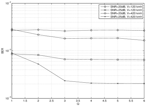
Finally, the BER performance of the proposed algorithm is presented as a function of $Q$ in Fig. 4. The parameter $Q$ can be chosen to trade off performance versus complexity. As a rule of thumb, we have seen that $Q=\lfloor f_{d_{max}}/\Delta f\rfloor+1$, where $f_{d_{max}}$ is the maximum Doppler frequency and $\Delta f$ is the subcarrier spacing, is an appropriate choice for Rayleigh fading[10]. In this paper, $f_{d_{max}}/\Delta f$ values are given as the normalized Doppler frequencies. It is concluded from these curves that the selection of the $Q$ value is highly dependent on SNR values. In particular, for $E_{b}/N_{0}=20dB$, different $Q$ values show similar performance because the effects of ICI are not very obvious relative to the effects of the additive Gaussian noise. The $Q$ value has a greater role for $Eb/N_{0}$ above 25dB because ICI is dominant. We note that $Q=3$ is sufficient for SNRs below 20dB.

V Conclusion

Conventional detection methods such as ZF and MMSE have irreducible error floors at high normalized Doppler frequency $f_{d}T_{s}$ since ICI corrupts the orthogonality among subcarriers. On the other hand, more sophisticated methods such as VBLAST require too much complexity, especially for large numbers of subcarriers. Therefore, we have proposed a new low-complexity maximum a posteriori probability (MAP) detection algorithm that provides excellent performance with manageable complexity for OFDM systems via the Gibbs sampling technique. In the simulation section, a comparison with other previously known receiver structures has been made and it has been demonstrated that MAP detection based on Gibbs sampling provides performance that is close to that of the optimal MAP detection algorithm for realistic fading conditions.

References

- [1] Q. Ni, A. Vinel, Y. Xiao, A. Turlikov, and T. Jiang, “Investigation of bandwidth request mechanisms under point-to-multipoint mode of WiMAX networks,” IEEE Commun. Mag., vol. 45, no. 5, pp. 132–138, 2007.
- [2] C. Eklund, R. Marks, K. Stanwood, and S. Wang, “IEEE standard 802.16: A technical overview of the WirelessMAN TM air interface for broadband wireless access,” IEEE Commun. Mag., vol. 40, no. 6, pp. 98–107, 2002.
- [3] H. Dogan, H. Cirpan, and E. Panayirci, “Iterative channel estimation and decoding of turbo coded SFBC-OFDM systems,” IEEE Trans. Wireless Commun., vol. 6, no. 8, pp. 3090–3101, 2007.
- [4] I. Barhumi, G. Leus, and M. Moonen, “Equalization for OFDM over doubly-selective channels,” IEEE Trans. Signal Process., vol. 54, no. 4, pp. 1445–1458, Apr. 2006.
- [5] A. Stamoulis, S. N. Diggavi, and N. Al-Dhahir, “Intercarrier interference in MIMO OFDM,” IEEE Trans. Signal Process., vol. 50, no. 10, pp. 2451–2464, Oct, 2002.
- [6] X. Huang and H.-C.Wu, “Robust and efficient intercarrier interference mitigation for OFDM systems in time-varying fading channels,” IEEE Trans. Veh. Technol., vol. 56, no. 5, pp. 2517–2528, Sep. 2007.
- [7] W. G. Jeon, K. H. Chang, and Y. S. Cho, “An equalization technique for orthogonal frequency-division multiplexing systems in time-variant multipath channels,” IEEE Trans. Commun., vol. 47, no. 1, pp. 27–32, Jan. 1999.
- [8] L. Rugini, P. Banelli, and G. Leus, “Simple equalization of time-varying channels for OFDM,” IEEE Commun. Lett., vol. 9, no. 7, pp. 619–621, Jul. 2005.
- [9] L. Rugini, P. Banelli, and G. Leus, “Low-complexity banded equalizers for OFDM systems in Doppler spread channels,” EURASIP Journal on Applied Signal Processing, vol. 2006, no. Article ID 67404, pp. 1–13, 2006.
- [10] P. Schniter, “Low-complexity equalization of OFDM in doubly-selective channels,” IEEE Trans. Signal Process., vol. 52, no. 4, pp. 1002–1011, Apr. 2004.
- [11] A. Gorokhov and J. P. Linnartz, “Robust OFDM receivers for dispersive time-varying channels: Equalization and channel acquisition,” IEEE Trans. Commun., vol. 52, no. 4, pp. 572–583, Apr. 2004.
- [12] Y.-S. Choi, P. J. Voltz, and F. A. Cassara, “On channel estimation and detection for multicarrier signals in fast and selective rayleigh fading channels,” IEEE Trans. Commun., vol. 49, no. 8, pp. 1375–1387, Aug. 2001.
- [13] X. Cai and G. B. Giannakis, “Bounding performance and suppressing intercarrier interference in wireless mobile OFDM,” IEEE Trans. Commun., vol. 51, no. 12, pp. 2047–2056, Dec. 2003.
- [14] S. Tomasin, A. Gorokhov, H. Yang, and J.-P. Linnartz, “Iterative interference cancellation and channel estimation for mobile OFDM,” IEEE Trans. Wireless Commun., vol. 4, no. 1, pp. 238–245, Jan. 2005.
- [15] S.-J. Hwang and P. Schniter, “Efficient sequence detection of multicarrier transmissions over doubly dispersive channels,” EURASIP J. Appl. Signal Process., vol. 2006, no. Article ID 93638, pp. 1–17, 2006.
- [16] S. Ohno and K. Teo, “Approximate BER expression of ML equalizer for OFDM over doubly selective channels,” in ICASSP 2008. IEEE International Conference on, 31 2008-April 4 2008, pp. 3049–3052.
- [17] B. F. Boroujeny, H. Zhu and Z. Shi, “Markov chain Monte Carlo Algorithms for CDMA and MIMO communication systems,” IEEE Trans. Signal Processing., vol. 54, no. 6, pp. 1896–1909, 2006.
- [18] C. Robert and G. Casella, Monte Carlo Statistical Methods. NewYork: Springer-Verlag, 1999.
- [19] S. Geman and D. Geman, “Stohastic relaxation, Gibbs distribution, and the Bayesian restoration of images,” IEEE Trans. Pattern Anal. Machine Intell., vol. PAMI 6, pp. 721–741, Nov 1984.