Triangles, squares and geodesics

Abstract.

In the early 1990s Steve Gersten and Hamish Short proved that compact nonpositively curved triangle complexes have biautomatic fundamental groups and that compact nonpositively curved square complexes have biautomatic fundamental groups. In this article we report on the extent to which results such as these extend to nonpositively curved complexes built out a mixture of triangles and squares. Since both results by Gersten and Short have been generalized to higher dimensions, this can be viewed as a first step towards unifying Januszkiewicz and Świȧtkowski’s theory of simplicial nonpositive curvature with the theory of nonpositively curved cube complexes.

1. Introduction

Many concepts in geometric group theory, including hyperbolic groups, $\textsc{CAT}(0)$ groups, and biautomatic groups, were developed to capture the geometric and computational properties of examples such as negatively curved closed Riemannian manifolds and closed topological $3$-manifolds. While the geometric and computational aspects of hyperbolic groups are closely interconnected, the relationship between the geometrically defined class of $\textsc{CAT}(0)$ groups and the computationally defined class of biautomatic groups is much less clear. Examples of biautomatic groups that are not $\textsc{CAT}(0)$ groups are known and there is an example of a $2$-dimensional piecewise Euclidean $\textsc{CAT}(0)$ group that is conjectured to be neither automatic nor biautomatic [5]. Nevertheless, several specific classes of $\textsc{CAT}(0)$ groups are known to be biautomatic, beginning with the following results by Gersten and Short [7].

Theorem 1.1 (Gersten-Short).

Every compact, nonpositively curved triangle complex has a biautomatic fundamental group. Similarly, every compact, nonpositively curved square complex has a biautomatic fundamental group.

We conjecture that this result extends to nonpositively curved complexes built out a mixture of triangles and squares.

Conjecture 1.2.

The fundamental group of a compact nonpositively curved triangle-square complex is biautomatic.

As progress towards answering Conjecture 1.2 in the affirmative, we establish that for every compact nonpositively curved triangle-square complex $K$ there exists a canonically defined language of geodesics that reduces to the regular languages used by Gersten and Short when $K$ is a triangle complex or a square complex. On the other hand, by investigating the canonical language of geodesics within a single flat plane, we highlight one reason why the “mixed” case studied here is significantly more difficult than the “pure” cases analyzed by Gersten and Short.

The article is structured as follows. The early sections review the necessary results about piecewise Euclidean complexes, nonpositively curved spaces, biautomatic groups, and disc diagrams. Sections 5 and 6 contain general results about combinatorial geodesics in $\textsc{CAT}(0)$ triangle-square complexes and Section 7 constructs the collection of canonical geodesic paths alluded to above. Sections 8, 9 and 10 investigate the behavior of these geodesics in a single triangle-square flat. Finally, Section 11 outlines the remaining steps needed to establish Conjecture 1.2.

2. Nonpositive curvature

We begin by reviewing the theory of nonpositively curved metric spaces built out of Euclidean polytopes. Although most of the article focuses on $2$-dimensional complexes where simplified definitions are available, the general definitions are given since higher dimensions occasionally occur. See [4] for additional details.

Definition 2.1 (Euclidean polytopes).

A Euclidean polytope $P$ is the convex hull of a finite set of points in a Euclidean space, or, equivalently, it is a bounded intersection of a finite number of closed half-spaces. A proper face of $P$ is a nonempty subset of $P$ that lies in the boundary of a closed half-space containing $P$. It turns out that every proper face of a polytope is itself a polytope. There are also two trivial faces: the empty face $\emptyset$ and $P$ itself. The interior of a face $F$ is the collection of its points that do not belong to a proper subface, and every polytope is a disjoint union of the interiors of its faces. The dimension of a face $F$ is the dimension of the smallest affine subspace that containing $F$. A $0$-dimensional face is a vertex and a $1$-dimensional face is an edge. A $2$-dimensional polytope is a polygon, and an $n$-gon if it has $n$ vertices.

Definition 2.2 (PE complexes).

A piecewise Euclidean complex (or PE complex) is the regular cell complex that results when a disjoint union of Euclidean polytopes are glued together via isometric identifications of their faces. A basic result due to Bridson is that so long as there are only finitely many isometry types of polytopes used in the construction, the result is a geodesic metric space, i.e. the distance between two points in the quotient is well-defined and achieved by a path of that length connecting them. This was a key result from Bridson’s thesis [3] and is the main theorem of Chapter I.7 in [4].

The examples under investigation are special types of PE $2$-complexes.

Example 2.3 (Triangle-square complexes).

A triangle complex is a PE complex where every polytope used in its construction is isometric to an equilateral triangle with unit length sides. Note that these complexes are not necessarily simplicial since two edges of the same triangle can be identified. They agree instead with Hatcher’s notion of a $\Delta$-complex [8]. Similarly, a square complex is a PE complex where every polytope used is a unit square and a triangle-square complex is one where every polytope used is either a unit equilateral triangle or a unit square.

Euclidean polytopes and PE complexes have spherical analogs that are needed for our characterization of nonpositive curvature.

Definition 2.4 (Spherical polytopes).

A spherical polytope is an intersection of a finite number of closed hemispheres in $\mathbb{S}^{n}$, or, equivalently, the convex hull of a finite set of points in $\mathbb{S}^{n}$. In both cases there is an additional requirement that the intersection or convex hull be contained in some open hemisphere of $\mathbb{S}^{n}$. This avoids antipodal points and the non-uniqueness of geodesics connecting them. With closed hemispheres replacing closed half-spaces and lower dimensional unit subspheres replacing affine subspaces, the other definitions are unchanged.

Definition 2.5 (PS complexes).

A piecewise spherical complex (or PS complex) is the regular cell complex that results when a disjoint union of spherical polytopes are glued together via isometric identifications of their faces. As above, so long as there are only finitely many isometry types of polytopes used in the construction, the result is geodesic metric space.

Definition 2.6 (Links).

Let $F$ be a face of a Euclidean polytope $P$. The link of $F$ in $P$ is the spherical polytope of unit vectors $u$ perpendicular to the affine hull of $F$ and pointing towards $P$ (in the sense that for any point $x$ in the interior of $F$ there is a sufficiently small positive value of $\epsilon$ such that $x+\epsilon u$ lies in $P$). For example, if $P$ is a polygon, and $F$ is one of its vertices, the link of $F$ in $P$ is a circular arc whose length is the radian measure of the interior angle at $F$, and if $F$ is an edge of $P$ then the link of $F$ in $P$ is a single point representing one of the two unit vectors perpendicular to the affine hull of $F$. Finally, when $K$ is a PE complex and $F$ is one of its cells, the link of $F$ in $K$ is the PS complex obtained by gluing together the link of $F$ in each of the various polytopal cells of $K$ containing it in the obvious way. When $F$ is a vertex, its link is a PS complex isometric (after rescaling) with the subspace of points distance $\epsilon$ from $F$. A vertex link in a triangle-square complex is a metric graph in which every edge either has length $\frac{\pi}{3}$ or $\frac{\pi}{2}$ depending on whether it came from a triangle or a square.

We turn now to curvature conditions. A $\textsc{CAT}(0)$ space is a geodesic metric space in which every geodesic triangle is “thinner” than its comparison triangle in the Euclidean plane and a space is nonpositively curved if every point has a neighborhood which is $\textsc{CAT}(0)$. A key consequence of the $\textsc{CAT}(0)$ condition is that every $\textsc{CAT}(0)$ space is contractible. For a PE complex these conditions are characterized via geodesic loops in its links.

Definition 2.7 (Geodesics and geodesic loops).

A geodesic in a metric space is an isometric embedding of a metric interval and a geodesic loop is an isometric embedding of a metric circle. A local geodesic and local geodesic loop are weaker notions that only require the image curves be locally length minimizing. For example, a path more than halfway along the equator of a $2$-sphere is a local geodesic but not a geodesic and a loop that travels around the equator twice is a local geodesic loop but not a geodesic loop. A loop of length less than $2\pi$ is called short.

Proposition 2.8 (Nonpositive curvature).

A PE complex with only finitely many isometry types of cells fails to be nonpositively curved iff it contains a cell whose link contains a short local geodesic loop, which is true iff it contains a cell whose link contains a short geodesic loop.

The first equivalence is the traditional form of Gromov’s link condition. The second follows because Brian Bowditch proved in [1] that when a link of a PE complex contains a short local geodesic loop, then some link (possibly a different one) contains a short geodesic loop. See [2] for a detail exposition of this implication. We record one corollary for future use.

Corollary 2.9.

Let $Y\to X$ be a cellular map between PE $2$-complexes that is an immersion away from the $0$-skeleton of $Y$ and an isometry on the interior of each cell. If $X$ is nonpositively curved then so is $Y$.

Proof.

First note that in a $2$-complex, the vertex links are the only links that can contain short local geodesic loops. Next, by hypothesis, the vertex links of $Y$ immerse into the vertex links of $X$ and, as a consequence, if $Y$ contains a vertex $v$ whose link contains a short local geodesic loop, then the link of $f(v)$ in $X$ contains a short local geodesic loop. Proposition 2.8 completes the proof. ∎

Proposition 2.10 ($\textsc{CAT}(0)$).

A PE complex with only finitely many isometry types of cells is $\textsc{CAT}(0)$ iff it is connected, simply connected, and nonpositively curved.

This follows from the Cartan-Hadamard Theorem: the universal cover of a complete, connected, nonpositively curved metric space is $\textsc{CAT}(0)$.

3. Biautomaticity

Biautomaticity involves distances in Cayley graphs and regular languages accepted by finite state automata. The standard reference is [6].

Definition 3.1 (Paths).

A path in a graph $\Gamma$ can be thought of either as an alternating sequence of vertices and incident edges, or as a combinatorial map $\alpha:I\to\Gamma$ from a subdivided interval $I$. Every connected graph can be viewed as a metric space by making each edge isometric to the unit interval and defining the distance between two points to be the length of the shortest path connecting them. In this metric the length of a path $\alpha$, denoted $|\alpha|$, is the number of edges it crosses. Define $\alpha(t)$ to be the start of $\alpha$ when $t$ is negative, the point $t$ units from the start of $\alpha$ when $0\leq t\leq|\alpha|$ and the end of $\alpha$ when $t>|\alpha|$.

Definition 3.2 (Distance).

Let $\alpha$ and $\beta$ be two paths in a graph $\Gamma$. There are two natural notions of distance between $\alpha$ and $\beta$. The subspace distance between $\alpha$ and $\beta$ is the smallest $k$ such that $\alpha$ (or more specifically its image) is contained in a $k$-neighborhood of $\beta$ and $\beta$ is contained in a $k$-neighborhood of $\alpha$. The path distance between $\alpha$ and $\beta$ is the maximum distance between $\alpha(t)$ and $\beta(t)$ as $t$ varies over all real numbers. When the path distance is bounded by $k$, $\alpha$ and $\beta$ are said to synchronously $k$-fellow travel.

For later use we note that when geodesics start close together, bounding their subspace distance also bounds their path distance.

Proposition 3.3 (Fellow travelling geodesics).

If $\alpha$ and $\beta$ are geodesic paths in $\Gamma$ that start distance $\ell$ apart, and the subspace distance between them is $k$, then the path distance between them is at most $2k+\ell$. In particular, they synchronously $(2k+\ell)$-fellow travel.

Proof.

Let $\alpha(t)$ be a point on $\alpha$ and let $\beta(t^{\prime})$ be the closest point on $\beta$. By hypothesis the distance between $\alpha(t)$ and $\beta(t^{\prime})$ is at most $k$. Moreover, because $\alpha$ and $\beta$ are geodesics, $t\leq t^{\prime}+k+\ell$ and $t^{\prime}\leq t+k+\ell$. Thus $|t-t^{\prime}|\leq k+\ell$. As a result, $\alpha(t)$ is within $k+(k+\ell)$ of $\beta(t)$. ∎

Definition 3.4 (Cayley graphs).

Let $K$ be a one-vertex cell complex with fundamental group $G$ and let $A$ index its oriented edges. The oriented loops indexed by $A$ represent a generating set for $G$ that is closed under involution and the $1$-skeleton of the universal cover of $K$ is called the right Cayley graph of $G$ with respect to $A$ and denoted $\textsc{Cay}(G,A)$. Alternatively, if $G$ is a group and $A$ is generating set closed under involution, $\textsc{Cay}(G,A)$ is a graph with vertices indexed by the elements of $G$ and an oriented edge connecting $v_{g}$ and $v_{g^{\prime}}$ labeled by $a$ whenever $g\cdot a=g^{\prime}$. Actually, the oriented edges come in pairs and we add only one unoriented edge for each such pair with a label associated with each orientation. It is the right Cayley graph because the generators multiply on the right. The second definition shows that the structure of $\textsc{Cay}(G,A)$ is independent of $K$. There is a natural label-preserving left $G$-action on $\textsc{Cay}(G,A)$ defined, depending on the definition, either by deck transformations or by sending $g\cdot v_{h}$ to $v_{g\cdot h}$.

Definition 3.5 (Languages).

An alphabet is a set $A$ whose elements are letters. A word is a finite sequence of letters, and the collection of all words is denoted $A^{*}$. A language $L$ over an alphabet $A$ is any subset of $A^{*}$. When $A$ is identified with the oriented edges of a one-vertex cell complex $K$ with fundamental group $G$, there are natural bijections between languages over $A$, collections of paths in $K$, and collections of paths in the universal cover of $K$ that are invariant under the $G$-action. A language $L$ over $A$ maps onto $G$ if the corresponding $G$-invariant set of paths contains at least one path connecting every ordered pair of vertices, or equivalently contains a word representing every element of $G$.

Two key properties of languages are used to define biautomatic groups.

Definition 3.6 (Regular languages).

A finite state automaton is a finite directed graph with decorations. The edges are labeled by a set $A$, there is a specified start vertex, and a subset of the vertices designated as accept states. Concatenating the labels on the edges of any path starting at the start vertex and ending at an accept state creates an accepted word. The collection of all accepted words is the language accepted by the automaton. Finally, a language is regular if it is accepted by some finite state automaton.

Definition 3.7 (Fellow travelling languages).

Let $G$ be a group generated by a finite set $A$ closed under inversion and let $L$ be a language over $A$ that maps onto $G$. The language $L$ fellow travels if there is a constant $k$ such that all pairs of paths in $\textsc{Cay}(G,A)$ that start and end at most $1$ unit apart and corresponding to words in $L$ synchronously $k$-fellow travel.

The following characterization of biautomaticity is from [6, Lemma 2.5.5].

Theorem 3.8 (Biautomaticity).

If $G$ is a group generated by a finite set $A$ closed under inversion and $L$ is a language over $A$ that maps onto $G$, then $L$ is part of a biautomatic structure for $G$ iff $L$ is regular and fellow travels.

Recall that a geometric action of a group on a space is one that is proper, cocompact and by isometries and note that the action of $G$ on its Cayley graph is geometric, but also free and transitive on vertices. By focusing on the paths in the Cayley graph corresponding to the language $L$ and slightly modifying a few definitions, Jacek Świa̧tkowski was able in [12] to extend the characterization of biautomaticity given in Theorem 3.8 to groups merely acting geometrically on a connected graph.

Definition 3.9 (Modified notions).

Let $G$ be a group acting geometrically on a connected graph $X$, and let $\mathcal{P}$ be a $G$-invariant collection of paths in $X$. The set $\mathcal{P}$ is said to map onto $G$ if every path start and ends in the $G$-orbit of a particular vertex $v$ and every ordered pair of vertices in the $G$-orbit of $v$ are connected by at least one path in $\mathcal{P}$. The $G$-invariant paths in $\mathcal{P}$ correspond to a set of paths in a finite graph (with loops when edges are inverted) and we say $\mathcal{P}$ is regular if the set of paths over the finite alphabet of oriented edges in the quotient is regular in the usual sense. Finally, the fellow traveler property is modified to consider pairs of paths that start and end within $\ell$ units of each other where $\ell$ has been chosen large enough so that any two vertices in the $G$-orbit of $v$ are connected by a sequence of other vertices in the orbit with adjacent vertices in the sequence at most $\ell$ units apart. When the $G$-orbit is vertex transitive, $\ell=1$ is sufficient.

Theorem 3.10 (Świa̧tkowski).

Let $G$ be a group acting geometrically on a connected graph $X$, and let $\mathcal{P}$ be a $G$-invariant collection of paths in $X$ that maps onto $G$. If $\mathcal{P}$ is regular and fellow travels in the modified sense described above, then $G$ is biautomatic.

4. Diagrams

The curvature of a PE $\textsc{CAT}(0)$ $2$-complex impacts the distances between paths in its $1$-skeleton via the reduced disc diagrams that fill its closed loops.

Definition 4.1 (Disc diagrams).

A disc diagram $D$ is a contractible $2$-complex with an implicit embedding into the Euclidean plane and a nonsingular disc diagram is a $2$-complex homeomorphic the closed unit disc $\mathbb{D}^{2}$. Disc diagrams that are not nonsingular are called singular and the main difference between the two is that singular disc diagrams contain cut points, i.e. points whose removal disconnects the diagram. The boundary of $D$ is a combinatorial loop that traces the outside of $D$ in a clockwise fashion. When $D$ is nonsingular, this is clear and when $D$ is singular amibiguities are resolved by the planar embedding. The boundary cycle is the essentially unique loop in $D$ that can be homotoped into $\mathbb{R}^{2}\setminus D$ while moving each point an arbitrarily small distance.

Definition 4.2 (Diagrams over complexes).

Let $D$ be a disc diagram and let $K$ be a regular cell complex. We say that a cellular map $f:D\to K$ turns $D$ into a disc diagram over $K$ and its boundary cycle is the image of the boundary cycle of $D$ under the map $f$. When a loop $\alpha$ in $K$ is the boundary cycle of a disc diagram $D$ over $K$ we say that $\alpha$ bounds $D$ and that $D$ fills $\alpha$.

Definition 4.3 (Reduced disc diagrams).

Let $f:D\to K$ be a disc diagram over a regular cell complex $K$. When there is a pair of $2$-cells in $D$ sharing an edge $e$ such that they are folded over along $e$ and identified under the map $f$, we say $D$ contains a cancellable pair and a disc diagram over $K$ with no cancellable pairs is said to be reduced. Note that a disc diagram over $K$ is a reduced disc diagram over $K$ iff the map $f:D\to K$ is an immersion away from the $0$-skeleton of $D$, which is true iff for every vertex $v$ in $D$, the induced map from the link of $v$ to the link of $f(v)$ is an immersion.

The importance of reduced disc diagrams over $2$-complexes derives from the following classical result. For a proof see [10].

Theorem 4.4 (Van Kampen’s Lemma).

Every combinatorial loop in a simply-connected regular cell complex bounds a reduced disc diagram.

In $2$-dimensions, curvature conditions on the cell complex $K$ propagate to reduced disc diagrams over $K$.

Corollary 4.5 ($\textsc{CAT}(0)$ disc diagrams).

Every combinatorial loop in a PE $\textsc{CAT}(0)$ $2$-complex bounds a PE $\textsc{CAT}(0)$ disc diagram.

Proof.

Let $\alpha$ be a combinatorial loop in a PE $\textsc{CAT}(0)$ $2$-complex $K$. Since $\textsc{CAT}(0)$ spaces are contractible, $\alpha$ bounds a reduced disc diagram $D$ by Theorem 4.4. By pulling back the metric of $K$ to $D$, we can turn it into a PE disc diagram. Next, by Corollary 2.9, $D$ is nonpositively curved. And finally, by Proposition 2.10 $D$ is $\textsc{CAT}(0)$. ∎

The fine structure of a PE $\textsc{CAT}(0)$ disc diagram is highlighted when we focus on its local curvature contributions.

Definition 4.6 (Angled $2$-complexes).

An angled $2$-complex is a $2$-complex $K$ where the corner of every polygon is assigned a number. When $K$ is PE, this number is naturally the measure of its angle, or equivalently the length of the spherical arc that is the link of this vertex in this polygon.

Definition 4.7 (Curvatures).

The curvature of a $n$-gon in an angled $2$-complex $K$ is the sum of its angles minus the expected Euclidean angle sum of $(n-2)\pi$. When $K$ is PE, its polygon curvatures are all $0$. The curvature of a vertex $v$ in an angled $2$-complex is $2\pi$ plus $\pi$ times the Euler characteristic of its link minus the sum of angles sharing $v$ as a vertex. When the angled $2$-complex is a disc diagram $D$ this reduces to $2\pi$ minus the angle sum for interior vertices and $\pi$ minus the angle sum for boundary vertices that are not cut points. Note that when $D$ is PE and nonpositively curved, the curvature of an interior vertex is nonpositive.

Theorem 4.8 (Combinatorial Gauss-Bonnet).

If $K$ is an angled $2$-complex then the sum of the vertex curvatures and the polygon curvatures is $2\pi$ times the Euler characteristic of $K$.

A proof of this relatively elementary result can be found in [10]. The basic idea is that every assigned angle contributes to exactly one vertex curvature and exactly one polygon curvature but with opposite signs. The curvature sum is thus independent of the angles assigned and minor bookkeeping equates it with $2\pi$ times the Euler characteristic. The main result we need is a easy corollary.

Corollary 4.9.

If $D$ is a PE $\textsc{CAT}(0)$ disc diagram, then the sum of its boundary vertex curvatures is at least $2\pi$.

Proof.

This follows from Theorem 4.8 once we note that being a disc diagram implies its Euler characteristic is $1$, PE implies its face curvatures are $0$ and $\textsc{CAT}(0)$ implies its interior vertex curvatures are nonnegative. ∎

5. Geodesics

In this section we use disc diagrams to turn an arbitrary path into a geodesic inside a $\textsc{CAT}(0)$ triangle-square complex. This procedure uses moves that modify paths by pushing across simple diagrams. After introducing these diagrams and moves, we describe the procedure.

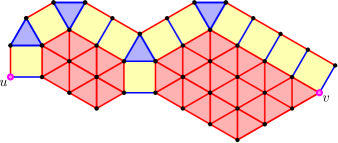
Definition 5.1 (Doubly-based disc diagrams).

A doubly-based disc diagram is a nonsingular disc diagram $D$ with two distinquished boundary vertices $u$ and $v$. An example is shown in Figure 1. The vertex $u$ is its start vertex and $v$ is its end vertex. When $u$ and $v$ are distinct there are two paths in the boundary cycle of $D$ that start at $u$ and end at $v$. The one that proceeds clockwise along the boundary is the old path and the one that proceeds counter-clockwise along the boundary is new path. When illustrating doubly-based diagrams, we place $u$ on the left and $v$ on the right so that the old path travels along the top and the new path travels along the bottom. The old path/new path terminology is extended to the case $u=v$ by defining the old path as the clockwise boundary cycle starting and ending at $u=v$ and the new path as the trivial path at $u=v$.

Figure 1. A doubly-based $\textsc{CAT}(0)$ disc diagram.

Definition 5.2 (Moves).

Let $\gamma$ be a path in a $2$-complex $K$ and let $D$ be a doubly-based disc diagram. If there is a map $D\to K$ that sends the old path to a directed subpath of $\gamma$, then applying the move $D$ means replacing the image of the old path in $\gamma$ with the image of the new path to create an altered path $\gamma^{\prime}$. This can be thought of as homotoping $\gamma$ across the image of $D$. The move is length-preserving when the old and new paths have the same length and length-reducing when the new path is strictly shorter.

The moves we are interested in are quite specific.

Definition 5.3 (Basic moves).

We define five basic types of moves over a triangle-square complex that involve a single triangle, a single square, a pair of triangles, a finite row of squares with a triangle on either end, or a single edge. We call these triangle moves, square moves, triangle-triangle moves, triangle-square-triangle moves, and trivial moves, respectively. Diagrams illustrating the first four are shown in Figure 2. Note that for each type of move the old path is at least as long as the new path. The triangle move is length-reducing. The start and end vertices for the square move are non-adjacent making it length-preserving. The start and end vertices of a triangle-triangle move or a triangle-square-triangle move are the unique vertices of valence $2$ and they are also length-preserving. Note that a triangle-square-triangle move can have any number of squares and that a triangle-triangle move can be viewed as degenerate triangle-square-triangle move with zero squares. Finally, the trivial move (defined below) is not a move in the sense of Definition 5.2, but it is included for convenience. Let $D$ be a diagram consisting of a single edge and identify both $u$ and $v$ with one of its vertices. If we view the path of length $2$ starting and ending at $u=v$ as the old path and the trivial path at $u=v$ as the new path, then we can view the removal of a “backtrack” in a path $\gamma$ as applying a trivial move across $D$.

Because the only moves considered from this point forward are the basic moves described above, we drop the adjective. Thus a move now refers to one of these five basic types. Notice that for every move (in this revised sense), the subspace distance between the old and new paths is $1$ since every vertex lies in one of the paths and, if not in both, it is connected to a vertex in the other path by an edge.

Figure 2. A triangle move, square move, triangle-triangle move and an example of a triangle-square-triangle move.

Definition 5.4 (Edges and paths).

Let $D$ be a nonsingular triangle-square disc diagram. Every boundary edge $e$ belongs to a unique $2$-cell in $D$ and we call $e$ a triangle edge or square edge depending on the type of this cell. Unless the boundary edges are all of one type, the boundary cycle of $D$ can be divided into an alternating sequence of maximal triangle edge paths and maximal square edge paths that we call triangle paths and square paths. Finally, a boundary vertex with positive curvature that is not the transition between a square path and a triangle path is said to be exposed.

The disc diagram shown in Figure 1 has $12$ triangle edges and $13$ square edges, its boundary is divided into $5$ triangle paths and $5$ square paths, and there are $4$ exposed vertices, one of which is $u$. Note that $v$ is not exposed even though its curvature is positive.

Lemma 5.5 (Exposed vertices).

If $D$ is a nonsingular triangle-square disc diagram with exposed vertex $v$, then a triangle move, square move, or triangle-triangle move can be applied to the boundary path of length $2$ with $v$ as its middle vertex.

Proof.

Because every angle in a triangle-square complex is $\frac{\pi}{3}$ or $\frac{\pi}{2}$, the possibilities for positive curvature are very limited. By nonsingularity there is at least one angle at $v$ but, if positively curved, there are at most two angles at $v$. The only possibilities are one triangle, one square, or two triangles. Two squares lead to nonpositive curvature and one of each only happens at the transitions between triangle and square paths. In each feasible case there is an obvious move. ∎

Definition 5.6 (Cumulative curvatures).

Let $D$ be a nonsingular triangle-square disc diagram $D$ with both triangle and square edges. The sum the curvatures of the boundary vertices along a square path in the boundary of $D$, including its endpoints, is called the cumulative curvature of this path.

If we let $\alpha$ and $\beta$ denote the old and new paths respectively of the doubly-based disc diagram shown in Figure 1, then the cumulative curvatures of its $5$ square paths (starting at $u$ and continuing clockwise) are $\frac{\pi}{2}$, $\frac{\pi}{3}$, $0$, $\frac{5\pi}{6}$ and $-\frac{\pi}{3}$. These add the curvatures from $\beta(1)$, $u$ and $\alpha(1)$, from $\alpha(2)$ and $\alpha(3)$, from $\alpha(4)$ through $\alpha(8)$, from $\alpha(9)$ through $v=\beta(11)$ and finally from $\beta(5)$ and $\beta(4)$, respectively.

Lemma 5.7 (Square paths).

If $D$ is a nonsingular triangle-square disc diagram and $\alpha$ is a square path in its boundary containing $k$ exposed vertices, then the cumulative curvature of $\alpha$ is at most $\frac{\pi}{3}+k\frac{\pi}{2}$. Moreover, if $\alpha$ contains no exposed vertices and has positive cumulative curvature, then a triangle-square-triangle move can be applied to a slight extension of $\alpha$.

Proof.

The endpoints of $\alpha$ have curvature at most $\frac{\pi}{6}$ (as they are incident with both a triangle and a square) and the interior vertices of $\alpha$ are either exposed with curvature $\frac{\pi}{2}$ or not exposed and nonpositively curved. The first assertion simply tallies these bounds. For the second, note that with no exposed vertices the cumulative curvature is at most $\frac{\pi}{3}$. If any unexpected angle (i.e. one that is not from a triangle or square that contains an edge of the path) is incident with a vertex of $\alpha$ then its cumulative curvature drops at least to $0$. And if no unexpected angles exist, $\alpha$ plus the triangle edges before and after form the old path of the triangle-square-triangle move whose $2$-cells are the cells of $D$ containing these boundary edges. ∎

The key result we need is the following.

Proposition 5.8 (Moves and basepoints).

If $D$ is a doubly-based nonsingular $\textsc{CAT}(0)$ triangle-square disc diagram, then a move can be applied to either the old path or the new path.

Proof.

If there is an exposed vertex distinct from $u$ and $v$, then Lemma 5.5 produces the required move. Note that this case already covers all diagrams without both triangle edges and square edges. With no transitions between triangle paths and square paths, every positively curved boundary vertex is exposed, its curvature is at most $\frac{2\pi}{3}$ and, since the total is at least $2\pi$ (Corollary 4.9), $D$ contains at least $3$ exposed vertices.

Next, if no exposed vertex distinct from $u$ and $v$ exists but there is a square path with positive cumulative curvature disjoint from $u$ and $v$, then Lemma 5.7 produces the required move. This second case covers all remaining diagrams, a fact we prove by contradiction.

Suppose $D$ is a diagram satisfying neither condition. Because $D$ contains both triangle edges and square edges, its boundary can be divided into triangle paths and square paths. Since there are no exposed vertices distinct from $u$ and $v$, every other vertex in the interior of a triangle path is nonpositively curved. By Corollary 4.9 the cumulative curvatures of the square paths plus the curvatures of the vertices in the interior of the triangle paths must be at least $2\pi$, but the only positive summands come from $u$, $v$ and/or the square paths that contains $u$, $v$ or both. Each possible configuration falls short. For example, if neither $u$ nor $v$ belong a square path, $u$ and $v$ each contribute at most $\frac{2\pi}{3}$ and there are no other positive summands. Similarly, if one basepoint belongs to a square path, but the other does not, then the square path containing the basepoint has cumulative curvature at most $\frac{\pi}{3}+\frac{\pi}{2}$ (Lemma 5.7), the other basepoint contributes at most $\frac{2\pi}{3}$ and there are no other positive summands. Next, if $u$ and $v$ belong the same square path, its cumulative curvature is at most $\frac{\pi}{3}+2\frac{\pi}{2}$ and there are no other positive summands. Finally, if $u$ and $v$ belong the distinct square paths, their cumulative curvatures are each at most $\frac{\pi}{3}+\frac{\pi}{2}$ and there are no other positive summands. In each case the total is less than $2\pi$, contradiction. ∎

Theorem 5.9 (Straightening paths).

Let $K$ be a $\textsc{CAT}(0)$ triangle-square complex and let $\alpha$ and $\beta$ be combinatorial paths in $K$ that start at $u$ and end at $v$, two not necessarily distinct vertices in $K$. When $\beta$ is a (possibly trivial) geodesic, $\alpha$ can be transformed into $\beta$ by a finite sequence of length-preserving and length-reducing moves. When both paths are geodesics, only length-preserving moves are needed.

Proof.

The proof proceeds by induction primarily on length and secondarily on area. More specifically, we show that for every coterminous pair of paths $\alpha$ and $\beta$, we can either apply a length-reducing move to $\alpha$, or a length-preserving move to $\alpha$ or $\beta$ so that the new pair of paths bounds a disc diagram with strictly fewer $2$-cells than the smallest diagram that $\alpha\beta^{-1}$ bounds. First the easy cases. If $\alpha=\beta$ there is nothing to prove. If $\alpha$ is not immersed then it can be shortened by a trivial move. If $\alpha$ is immersed but not embedded then a closed proper subpath $\alpha^{\prime}$ can be paired with a trivial path satisfying the induction hypothesis. (The path $\beta$ is always immersed and embedded because it is geodesic.) Similarly, if $\alpha$ and $\beta$ share internal vertices, then we can split $\alpha$ into $\alpha_{1}\alpha_{2}$ and $\beta$ into $\beta_{1}\beta_{2}$ where $\alpha_{i}$ and $\beta_{i}$ are shorter paths satisfying the induction hypothesis.

In the remaining case, $\alpha\beta^{-1}$ bounds a $\textsc{CAT}(0)$ disc diagram $D$ (Corollary 4.5) and the restrictions on $\alpha$ and $\beta$ force $D$ to be nonsingular. By Proposition 5.8 there is either a length-reducing or length-preserving diagram-shrinking move that avoids the distinguished vertices $u$ and $v$. This is sufficient since length-preserving moves can only occur a bounded number of times before one of the easy cases or a length-reducing move occurs. Finally, since $\beta$ is a geodesic, the modifications to $\beta$ and its descendents only involve length-preserving moves. Thus, the modifications can be reordered so that all the alterations to paths descended from $\alpha$ happen first, followed by the alterations to the paths descended from $\beta$ in reverse (and in reverse order) to complete the process. ∎

6. Intervals

We now shift our attention from a single geodesic to the global structure of all geodesics connecting fixed vertices in a $\textsc{CAT}(0)$ triangle-square complex.

Figure 3. A doubly-based $\textsc{CAT}(0)$ disc diagram with the corresponding interval heavily shaded.

Definition 6.1 (Intervals).

Let $u$ and $v$ be fixed vertices in a $\textsc{CAT}(0)$ triangle-square complex $K$ that are distance $n$ apart in the $1$-skeleton metric. We say a vertex $w$ is between $u$ and $v$ when $w$ lies on a combinatorial geodesic connecting $u$ to $v$ or, equivalently, when $d(u,w)+d(w,v)=d(u,v)$. The interval between $u$ and $v$, denoted $K[u,v]$, is the largest subcomplex of $K$ with all vertices between $u$ and $v$, i.e. the full subcomplex on this vertex set. More explicitly, it includes all vertices between $u$ and $v$, all of the edges of $K$ connecting them, and every triangle or square in $K$ with all of its vertices in this set. Note that $K[u,v]$ contains every geodesic from $u$ to $v$ as well as every length-preserving move that converts one such geodesic into another one. An example of an interval is shown in Figure 3.

Remark 6.2 (Planar and locally Euclidean).

Examples that are planar and locally Euclidean can be illustrated with undistorted metrics but neither of these properties hold in general for intervals in $\textsc{CAT}(0)$ triangle-square complexes. See Figure 4. This is one place where the “mixed” case is very different from the “pure” cases. Gersten and Short proved, at least implicitly, that intervals in $\textsc{CAT}(0)$ square complexes can always be identified with subcomplexes of the standard square tiling of $\mathbb{R}^{2}$ and that intervals in $\textsc{CAT}(0)$ triangle complexes can always be identified with subcomplexes of the standard triangle tiling of $\mathbb{R}^{2}$. In particular they are always planar and locally Euclidean. In fact, B. T. Williams proved in his dissertation that an analogous result holds for $n$-dimensional cube complexes and the standard cubing of $\mathbb{R}^{n}$ [13].

Figure 4. An interval that is not planar and another that is not locally Euclidean.

Despite these complications, an interval in a $\textsc{CAT}(0)$ triangle-square complex is still a highly structured object. As we now show, it is a simply-connected $\textsc{CAT}(0)$ subcomplex in which every edge of its $1$-skeleton belongs to a either a geodesic or a move. We begin with a definition.

Definition 6.3 (Vertical and horizontal edges).

Let $K[u,v]$ be an interval in a $\textsc{CAT}(0)$ triangle-square complex $K$ and let $x$ and $y$ be vertices in $K[u,v]$ connected by an edge $e$. We call $e$ a horizontal edge of $K[u,v]$ when $x$ and $y$ are the same distance from $u$ (and consequently the same distance from $v$) and a vertical edge otherwise.

Lemma 6.4 (Edges in intervals).

Let $K[u,v]$ be interval in a $\textsc{CAT}(0)$ triangle-square complex $K$. Every edge in the interval either lies on a geodesic from $u$ to $v$ or is part of a move between two such geodesics. More specifically, vertical edges lies on geodesics and horizontal edges are contained in moves.

Proof.

Let $e$ be an edge connecting $x$ and $y$ in $K[u,v]$. Because $x$ and $y$ are in $K[u,v]$ they lie on geodesics $\alpha$ and $\beta$ and can be viewed as $x=\alpha(i)$ and $y=\beta(j)$ for integers $i$ and $j$. These integers also represent the distance $x$ and $y$ are from $u$, respectively. The difference between $i$ and $j$ is at most $1$ because otherwise, we could use one end of $\alpha$, $e$ and the other end of $\beta$ to construct a new path shorter than the geodesics $\alpha$ and $\beta$. As it is, if $i+1=j$, the path that follows $\alpha$ from $u$ to $x=\alpha(i)$, crossses $e$, and then follows $\beta$ from $y=\beta(j)$ to $v$ is a geodesic containing $e$.

When $e$ is horizontal, add a new triangle to $K$ along $e$ with third vertex $z$. It is easy to check that the augmented complex remains $\textsc{CAT}(0)$ and that there are geodesics $\alpha_{1}$ and $\beta_{1}$ from $u$ to $z$ through $x$ and $y$, respectively. By Theorem 5.9 there is a finite sequence of length-preserving moves that transforms $\alpha_{1}$ to $\beta_{1}$ inside the augmented complex. Since the only $2$-cell that contains $z$ is a triangle any move that converts a geodesic through $x$ to a geodesic through $y$ must be a (possibly degenerate) triangle-square-triangle move. In particular, $K[u,v]$ contains a triangle-square-triangle move minus its final triangle pointing towards $u$ and ending at $e$. After repeating this argument focusing on the beginning of the interval $K[z,v]$, we can merge the two uncapped triangle-square-triangle moves containing $e$, one pointing towards $u$ and the other towards $v$, into a triangle-square-triangle move inside $K[u,v]$ that contains $e$. ∎

Theorem 6.5 (Intervals are $\textsc{CAT}(0)$).

Intervals in $\textsc{CAT}(0)$ triangle-square complexes are simply-connected and thus $\textsc{CAT}(0)$.

Proof.

Let $K[u,v]$ be an interval in a $\textsc{CAT}(0)$ triangle-square complex $K$. As a subcomplex of a $\textsc{CAT}(0)$ PE $2$-complex, $K[u,v]$ is nonpositively curved by Corollary 2.9. Once we establish that it is simply-connected, $\textsc{CAT}(0)$ follows by Proposition 2.10. Let $\gamma$ be a closed combinatorial path in $K[u,v]$. Using Lemma 6.4 we can embed each edge in $\gamma$ in either a geodesic from $u$ to $v$ or a move connecting two such geodesics. Theorem 5.9 can then be used to fill in the gaps between these geodesics and the geodesics on either side of these moves in such a way that there is a map $\mathbb{S}^{2}\to K[u,v]$ sending the south pole to $u$, the north pole to $v$, the equator to $\gamma$ (with constant maps inserted between the edges), longitude lines to geodesics and lunes between the adjacent longitude lines alternately to the diagrams provided by Theorem 5.9 and the geodesic or move containing a particular edge of $\gamma$. The image of the southern hemisphere under this map shows that $\gamma$ is null-homotopic and $K[u,v]$ is simply-connected. ∎

7. Gersten-Short geodesics

In this section we define a collection of paths in a $\textsc{CAT}(0)$ triangle-square complex that reduces to the paths chosen by Gersten and Short in $\textsc{CAT}(0)$ triangle complexes and in $\textsc{CAT}(0)$ square complexes. The first step is to show that all geodesics from $u$ to $v$ either contain a common first edge or there is a unique nontrivial move in the interval starting at $u$.

Proposition 7.1 (Unique $2$-cell).

If both the old path and the new path of a doubly-based nonsingular $\textsc{CAT}(0)$ triangle-square disc diagram $D$ are geodesics, then the start vertex of $D$ lies in the boundary of a unique $2$-cell.

Proof.

Suppose not and select a counterexample that is minimal in the following sense. First minimize the distance between the basepoints and then minimize the number of $2$-cells in $D$. Any move that can be applied to either path in such a minimal counterexample must contain the vertex $u$ as an endpoint since applying a move not containing $u$ either produces a counterexample with fewer $2$-cells or a singular diagram containing a counterexample whose basepoints are closer together.

If all boundary edges of $D$ are square edges, then every positively curved boundary vertex is exposed with curvature $\frac{\pi}{2}$. To reach $2\pi$ (Corollary 4.9) there must be at least $4$ such vertices. Since $u$ itself is not exposed, there exists an exposed vertex distinct from $u$, $v$ and the vertices adjacent to $u$, but this leads to a square move contradicting the minimality of $D$ (Lemma 5.5). Thus triangle edges exist in $D$.

Next, add the boundary vertex curvatures of $D$ so that the curvature of each boundary vertex not touching a square edge is an individual summand and the curvature of vertices in square paths are collected together into cumulative curvature summands. The total is at least $2\pi$ (Corollary 4.9), but the only positive summands come from $u$ and $v$ (and/or the square paths that contain them) and from moves that contain $u$ as an endpoint since other positive terms lead to moves that contradict the minimality of $D$ (Lemmas 5.5 and 5.7).

When both boundary edges touching $u$ are triangle edges, the curvature of $u$ is at most $\frac{\pi}{3}$ and any move with $u$ as an endpoint is a (possibly degenerate) triangle-square-triangle move with cumulative curvature at most $\frac{\pi}{3}$. Note that there are at most two such moves, one in each path. Finally, the curvature of $v$ or the cumulative curvature of the square path containing $v$ is at most $\frac{5\pi}{6}$, the extreme case being $v$ exposed in the middle of a square path. These are the only possible sources of positive curvature and their total is bounded by $\frac{11\pi}{6}<2\pi$, contradiction.

Next, suppose $u$ and $v$ belong the same square path. If $u$ is not an endpoint, then the only positive summand is the cumulative curvature of this square path. Moreover, its curvature is at most $\frac{\pi}{3}+3\cdot\frac{\pi}{2}$ (Lemma 5.7) since the $v$ and the two vertices adjacent to $u$ are the only ones that can be exposed. If $u$ and $v$ belong to the same square path and $u$ is an endpoint, then the only positive summands are the cumulative curvature of this square path and a possible triangle-square-triangle move ending at $u$. These curvatures are bounded by $\frac{\pi}{3}+2\cdot\frac{\pi}{2}$ and $\frac{\pi}{3}$, respectively. Both totals are less than $2\pi$, contradiction.

Finally, suppose $u$ belongs to a square path that does not include $v$. As above, the curvature of $v$ or the cumulative curvature of the square path containing $v$ is at most $\frac{5\pi}{6}$, with the extreme case being $v$ exposed in the middle of a square path. Thus it suffices to show that the curvatures associated with $u$ are at most $\pi$. If $u$ is not an endpoint of the square path, then $u$ itself is nonpositively curved and total curvature of the path on either side is bounded by $\frac{\pi}{3}$. To see this note that an easy bound is $\frac{\pi}{6}+\frac{\pi}{2}$, the first term from a positively curved endpoint and the second from a single exposed vertex adjacent to $u$, but if there are no unexpected angles along the path, then this leads a configuration that violates our assumption that both boundary paths from $u$ to $v$ are geodesics. Thus the improved bound is $\frac{\pi}{6}+\frac{\pi}{2}-\frac{\pi}{3}=\frac{\pi}{3}$. And if $u$ is endpoint, then the cumulative curvature of the square path excluding $u$ is bounded by $\frac{\pi}{3}$ using the argument just given. The curvature of $u$ is at most $\frac{\pi}{6}$ and the triangle-square-triangle move ending at $u$, if it exists, has curvature at $\frac{\pi}{3}$. Thus, all configurations lead to totals less than $2\pi$. ∎

Proposition 7.2 (Initial link).

If $u$ and $v$ are distinct vertices in a $\textsc{CAT}(0)$ triangle-square complex $K$, then the link of $u$ in the interval $K[u,v]$ is either a single vertex or a single edge.

Proof.

Every pair of distinct vertices in the link corresponds to edges leaving $u$ that can be extended to geodesics $\alpha$ and $\beta$ from $u$ to $v$. From these geodesics Theorem 5.9 implicitly constructs a path in the link connecting the original vertices. In fact, by Corollary 4.9 there is a $\textsc{CAT}(0)$ disc diagram $D$ filling $\alpha\beta^{-1}$. After restricting our attention to a nonsingular subdiagram containing $u$ if necessary, Proposition 7.1 shows that there is a $2$-cell in $D$ touching $u$ providing an edge in the link connecting the two original vertices. If the link contains three distinct vertices, then edges connect them to form a triangular geodesic loop that is short since each edge has length at most $\frac{\pi}{2}$. This is impossible because $K[u,v]$ is $\textsc{CAT}(0)$ (Theorem 6.5). Finally, loops of length $1$ and multiple edges are prohibited in the link for similar reasons. ∎

Theorem 7.3 (First move).

If $u$ and $v$ are distinct vertices in a $\textsc{CAT}(0)$ triangle-square complex $K$, then either every geodesic from $u$ to $v$ has the same first edge or there are exactly two possible first edges and there is a unique move in $K[u,v]$ that contains both of them.

Proof.

When the link of $u$ in $K[u,v]$ is a single vertex, then the corresponding edge in $K[u,v]$ is the first edge in every geodesic from $u$ to $v$. The only other possibility, according to Proposition 7.2 is that the link of $u$ in $K[u,v]$ is a single edge. In this case the vertex $u$ lies in the boundary of a unique $2$-cell and both edges adjacent to $u$ can be extended to geodesics from $u$ to $v$. That this $2$-cell is part of some move in $K[u,v]$ is a consequence of Theorem 5.9. To see uniqueness, suppose there were two such moves and focus on the $2$-cells closest to $u$ that are in one move but not the other. Using Proposition 7.2 to fill in gaps between vertical edges with a common start vertex it is easy to construct a short loop in its link, contradicting the fact that $K[u,v]$ is $\textsc{CAT}(0)$. ∎

Definition 7.4 (Gersten-Short geodesics).

Let $u$ and $v$ be vertices in a $\textsc{CAT}(0)$ triangle-square complex $K$. A Gersten-Short geodesic from $u$ to $v$ is defined inductively using Theorem 7.3. If $u=v$ then the only geodesic is the trivial path. When $u$ and $v$ are distinct there are two possibilities. If every geodesic from $u$ to $v$ has the same first edge then the Gersten-Short geodesic travels along this edge to its other endpoint $u^{\prime}$, and if there is a unique move in $K[u,v]$ that contains the two possible first edges, then we travel along either side of this unique move to its other endpoint $u^{\prime}$. In either case, the new vertex $u^{\prime}$ is closer to $v$ and the rest of the path is an inductively defined Gersten-Short geodesic from $u^{\prime}$ to $v$. The vertex $u^{\prime}$ is called the first choke point of $K[u,v]$. If we let $u_{0}=u$ and define $u_{i+1}$ as the first choke point of $K[u_{i},v]$ then eventually $u_{i}=v$. These $u_{i}$’s are the choke points between $u$ and $v$ and every Gersten-Short geodesic from $u$ to $v$ goes through each one.

Figure 5. The choke points of the Gersten-Short geodesics in an interval.

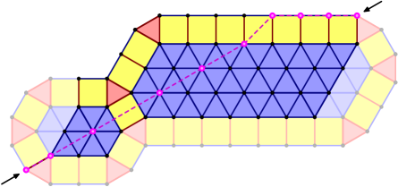
Example 7.5 (Gersten-Short geodesics).

Figure 5 shows the series of choke points in an interval used to define its Gesten-Short geodesics. When the dotted line connecting two choke points runs along an edge, this edge belongs to all of the Gersten-Short geodesics between $u$ and $v$. When it cuts through a number of $2$-cells, these $2$-cells form the unique next move and every Gersten-Short geodesic runs along one side or the other. In the example, there are, in order, an edge, a triangle-triangle move, a triangle-square-triangle move, two more triangle-triangle moves, a square move and finally three edges. Because there are $5$ moves involved there are $2^{5}=32$ Gersten-Short geodesics.

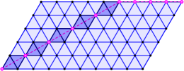
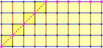
Example 7.6 (Pure complexes).

When $K$ is a $\textsc{CAT}(0)$ triangle complex or a $\textsc{CAT}(0)$ square complex, its intervals look like subcomplexes of the standard square and triangular tilings of $\mathbb{R}^{2}$, respectively. It is thus instructive to consider what intervals and Gersten-Short geodesics look like when $K$ itself is one of these tilings. Nonsingular intervals in this special case look like parallelograms and rectangles and the choke points of typical Gersten-Short paths are shown in Figure 6. In simple examples such as these it is easy to see the directed nature of the definition. The Gersten-Short geodesics from $v$ to $u$ are definitely different.

Figure 6. The choke points of Gersten-Short geodesics in intervals of the standard triangle and square tilings of $\mathbb{R}^{2}$.

It is important to remark, that in these pure cases, the paths that we have identified are essentially the same paths that Gersten and Short identified in [7]. The only difference is that they added extra restrictions so that a unique geodesic is selected between every pair of endpoints $u$ and $v$. This difference is insignificant because of the following result which is an immediate corollary of the definition and the fact that the two sides of a length-preserving move $1$-fellow travel.

Corollary 7.7 ($1$-fellow travel).

The Gersten-Short geodesics from $u$ to $v$ in a $\textsc{CAT}(0)$ triangle-square complex $K$ pairwise $1$-fellow travel.

8. Flats

Now that we have established the existence of a language of geodesic paths that generalizes the regular language of geodesics used by Gersten and Short, we shift our attention to flats, the main obstacles to establishing biautomaticity.

Definition 8.1 (Flats).

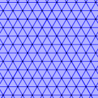
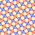
A triangle-square flat is a triangle-square complex isometric to the Euclidean plane $\mathbb{E}=\mathbb{R}^{2}$. Suggestive portions of several triangle-square flats are shown in Figure 8. More generally, a flat is any metric space isometric to a Euclidean space $\mathbb{R}^{n}$, with $n$ at least $2$, and a flat in a metric space $K$ is a flat $F$ together with an isometric embedding $F\to K$. When $F$ is a triangle-square flat and $K$ is a triangle-square complex we further insist that the embedding is a cellular map.

The importance of flats is highlighted by the following result.

Theorem 8.2 (Flats and biautomaticity).

Let $K$ be a compact nonpositively curved PE complex. If the universal of $K$ does not contain an isometrically embedded flat plane, then $\widetilde{K}$ is $\delta$-hyperbolic, $\pi_{1}(K)$ is word hyperbolic, and thus $\pi_{1}(K)$ is biautomatic.

Proof.

These assertions follow from the flat plane theorem [4], the definition of word hyperbolicity, and the fact, proved in [6], that every word hyperbolic group is biautomatic. ∎

More generally, Chris Hruska has shown in [9] that any group that acts geometrically on a $\textsc{CAT}(0)$ $2$-complex with the isolated flats property is biautomatic. For $\textsc{CAT}(0)$ $2$-complexes, the isolated flats property is the same as the non-existence of an isometric embedding of a triplane, a triple of upper half-planes sharing a common boundary line. Thus, if $\widetilde{K}$ contains no flats (or if those that do exist are isolated), then $\pi_{1}(K)$ is already known to be biautomatic. In particular, when biautomaticity fails, it fails directly or indirectly because of the flats in $\widetilde{K}$. When analyzing a flat, we begin by decomposing it into regions.

Definition 8.3 (Regions).

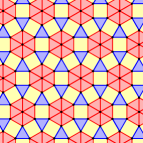
Let $F$ be a triangle-square flat and consider the equivalence relation on its $2$-cells generated by placing $2$-cells in the same equivalence class when they are the same type and share an edge. The union of the closed $2$-cells in an equivalence class is called a region of $F$ and it is triangular or square depending on the type of $2$-cell it contains. For example, the flat in the lower lefthand corner of Figure 8 has six visible triangular regions and five square regions.

The next step is to observe that these regions are convex, based on the strong local restrictions that vertices in triangle-square flats must satisfy.

Figure 7. Four possible vertex neighborhoods in a flat.

Definition 8.4 (Vertices in flats).

A vertex $v$ in a triangle-square flat $F$ is surrounded by corners whose angles total $2\pi$ and the possibilities are extremely limited. If $v$ lies in the interior of a region then it is either surrounded by $6$ triangles or by $4$ squares. The only other possibility is that there are $3$ triangles and $2$ squares touching $v$ and they are arranged in one of two distinct ways. When the two squares are adjacent, we say $v$ is along a side and when they are not, $v$ is a corner of a region. See Figure 7.

In each local configuration, the boundaries of the represented regions are locally convex and thus every region is (globally) convex. When analyzing more complicated triangle-square flats, it is useful to introduce a color scheme to highlight additional features.

Definition 8.5 (Colors).

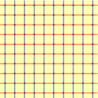
Let $F$ be a triangle-square flat and assume it has been oriented so that at least one of its edges is vertical or horizontal. The restrictive nature of the angles involved means that for every edge $e$ in $F$, the line $\ell$ containing $e$ points in one of six directions. Concretely, the angle from horizontal is a multiple of $\frac{\pi}{6}$. We divide the edges of $F$ into two classes based on the parallelism class of the lines containing them. If the line containing $e$ is horizontal (or forms a $\frac{\pi}{3}$ angle with a horizontal line) then it is a blue edge. If the line containing $e$ is vertical (or forms a $\frac{\pi}{3}$ angle with a vertical line) then it is a red edge. Under these definitions, the six possible parallelism classes alternate between red and blue. Note that all three edges of a triangle receive the same color so that it makes sense to speak of red triangles and blue triangles. The edges of a square, on the other hand, alternate in color. Being neither red nor blue, squares are assigned a third color such as yellow. (For those viewing an electronic version of this article, we have followed these coloring conventions in all of our illustrations.) When $F$ is oriented so that our color conventions apply, we say that $F$ is colored.

Figure 8. Six examples of triangle-square flats. They are pure triangle, pure square, striped, radial, and a pair of thoroughly crumpled flats. The radial flat is intrinsically aperioidic; the other five are potentially periodic.

Definition 8.6 (Types of flats).

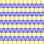
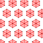
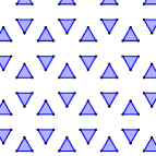
Let $F$ be a triangle-square flat. If $F$ contains only triangles or only squares, we say that $F$ is pure. If $F$ contains both triangles and squares but it contains no corner vertices, then $F$ is striped. If $F$ contains a corner vertex and at least one region that is unbounded, then $F$ is radial. Finally, if every region of $F$ is bounded, then $F$ is crumpled and if there is a uniform bound on the number of $2$-cells in a region of $F$, we say $F$ is thoroughly crumpled. Several examples are shown in Figure 8).

The reason that impure flats with no corners are called striped planes is explained by the following observation.

Lemma 8.7 (Striped flats).

Let $F$ be a triangle-square flat. If one region of $F$ has a straight line as part of its boundary then every region of $F$ is bounded by parallel straight lines. In particular, a triangle-square flat is striped iff it contains a region with a straight line as part of its boundary, which is true iff every region is an infinite strip or a half-plane.

Proof.

Let $R$ be the region with a straightline as part of its boundary. If this is all of its boundary then $R$ is a half-plane. If it is not all of its boundary then the convexity of $R$ forces the remaining portion to be a parallel straightline (since corners lead to contradictions to convexity and nonparallel straight lines would intersect). In other words, $R$ must be an infinite strip, an interval cross $\mathbb{R}$. Shifting our the region on the other side of a boundary line of $R$ we see that it too is either a half-plane or a strip and we can continue in this way until the entire plane is exhausted. The final assertion is now nearly immediate. If $F$ has both triangles and squares but no corner vertices then there is an edge bordering both a triangle and a square and it must extend to a straight line boundary between regions. As argued above, it follows that every region is then an infinite strip or a half-plane. Conversely, when every region is either a half-plane or an infinite strip, the flat clearly contains both triangles and squares and no corner vertices. ∎

As a corollary of Lemma 8.7 note that the obvious flats embedded in a triplane must be pure or striped since triplanes are formed from three tiled half-planes with a common boundary. The wide variety of cell structures exhibited by triangle-square flats is the key difficulty encountered when trying to extend results from pure triangle and pure square complexes to mixed triangle-square complexes. This is in sharp contrast with the pure situation since every flat in a triangle complex or in a square complex is obviously pure.

Definition 8.8 (Pure flats).

A pure triangle-square flat of either type is essentially unique in that it must look like the standard tiling of $\mathbb{R}^{2}$ by triangles or a standard tiling by squares. Because the vertex sets of pure flats can be identified with the Eisenstein integers $\mathbb{Z}[\omega]$ in the triangle case or the Gaussian integers $\mathbb{Z}[i]$ in the square case (where $\omega$ and $i$ are primitive third and fourth roots of unity), we call these complexes Eisenstein and Gaussian planes, respectively, and denote them $\mathcal{E}$ and $\mathcal{G}$.

One illustration of the variety available in the mixed case, is the existence of flats that are intrinsically aperiodic.

Definition 8.9 (Intrinsically aperiodic flats).

Let $K$ be a complex and let $F$ be a flat that embeds into its universal cover $\widetilde{K}$. Composition with the covering projection immerses $F$ into $K$ itself and it is traditional to call $F$ periodic or aperiodic depending on whether or not this immersion $F\to K$ factors through metric Euclidean torus. This is equivalent to finding a subgroup isomorphic to $\mathbb{Z}\times\mathbb{Z}$ in $\pi_{1}(K)$ so that the corresponding deck transformations of $\widetilde{K}$ stabilize the image of $F$ setwise and act cocompactly on this image. For our purposes we need a different distinction that is intrinsic to $F$ itself. We say that $F$ is potentially periodic if there exists a cocompact $\mathbb{Z}\times\mathbb{Z}$ action on $F$ by cellular maps and intrinsically aperiodic if no such action exists. We should note that by passing to a finite-index subgroup if necessary, we can always insist that the $\mathbb{Z}\times\mathbb{Z}$ action on $F$ consists solely of translations.

Only certain types of flats can be potentially periodic.

Proposition 8.10 (Potentially periodic flats).

Every potentially periodic triangle-square flat is pure, striped or thoroughly crumpled.

Proof.

Let $F$ be a potentially periodic triangle-square flat. By assumption there is a cocompact action of $\mathbb{Z}\times\mathbb{Z}$ on $F$. Let $n$ be the number of vertices in a fundamental domain for this action and note that regions are sent to regions under this cellular action. If $F$ is not thoroughly crumpled, it contains a region $R$ with more than $n$ vertices, which implies that there is a non-trivial translation of $F$ that sends $R$ to $R$. In particular, $R$ is a convex subset of $\mathbb{R}^{2}$ that is invariant under a non-trivial translation. Unless $F$ is pure, this means that $R$ contains a straightline as part of its boundary and by Lemma 8.7, the flat $F$ is striped. ∎

9. Geodesics in flats

As a first step towards showing that the Gersten-Short geodesics can be used to define biautomatic structures, consider the following question. Suppose that $F$ is a triangle-square flat viewed as a $\textsc{CAT}(0)$ triangle-square complex in its own right. Does there exists a universal constant $k$, possibly depending on the structure of $F$, such that every pair of Gersten-Short paths in $F$ that start and end at most $1$ unit apart synchronously $k$-fellow travel? The answer, unfortunately, is that this is true for certain types of flats (such as pure flats and striped flats) but it is definitely not true in general. In other words, this is an instance where new phenomena are produced when triangles and squares are mixed. We begin by showing that Gersten-Short paths in pure flats and striped flats are well-behaved.

Proposition 9.1 (Fellow traveling in pure flats).

If $F$ is a pure triangle or pure square flat, then pairs of Gersten-Short geodesics in $F$ that start and end within $1$ unit of each other synchronously $k$-fellow travel for a small explicit value of $k$.

Proof.

Let $F$ be a pure square flat and let $\alpha$ be a Gersten-Short geodesic from $u$ to $v$. Because the structure of $F$ is so simple, we know that the choke points initially jump across a (possibly empty) sequence of square moves, followed by a (possibly empty) sequence of unique edges. In particular, if we arrange $F$ so that its edges are horizontal/vertical and then connect the successive choke points with straight segments, the result is a pair of line segments approximating $\alpha$ where the first has slope $\pm 1$ and the second is either horizontal or vertical. See Figure 6. If $\beta$ is a second Gersten-Short geodesic that starts within $1$ unit of $u$ and ends within $1$ unit of $v$, the same procedure will produce a pair of line segments with the same slopes and in the same configuration (unless one of the two original segments is very short). In particular, every choke point of $\alpha$ is connected to a choke point of $\beta$ by an edge and vice versa. Since every vertex in $\alpha$ or $\beta$ is within $1$ unit of a choke point, the subspace distance between the two paths is at most $3$ and by Proposition 3.3, $\alpha$ and $\beta$ synchronously $7$-fellow travel. (With a bit more work one can show that $\alpha$ and $\beta$ synchronously $3$-fellow travel, but it is the existence of a bound that is significant.) The argument for Gersten-Short geodesics in pure triangle flats is essentially identical. ∎

A similar result can be established for geodesics in striped flats.

Figure 9. Two examples of intervals in striped flats and a subdivision of the squares in the second example as described in the proof of Proposition 9.2.

Proposition 9.2 (Fellow traveling in striped flats).

If $F$ is a striped flat, then pairs of Gersten-Short geodesics in $F$ that start and end within $1$ unit of each other synchronously $k$-fellow travel for a small explicit value of $k$.

Proof.

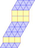
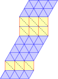
Let $F[u,v]$ be an interval in a striped flat $F$ between vertices $u$ and $v$. If $F$ is arranged so that the boundaries between regions are horizontal, then $F[u,v]$ can viewed as an interval in a pure triangle flat, i.e. a (possibly degenerate) triangulated parallelogram, with with horizontal square strips inserted. Two possibilities are illustrated in Figure 9. The key difference between the two examples is whether the edges that lie on the boundary between a triangular region and a square region are “horizontal” or “vertical” in the terminology of Definition 6.3. When one of these boundary edges is “horizontal”, they are all “horizontal” and every square in a square region of $F[u,v]$ is part of a triangle-square-triangle move where the line segment connecting the choke points at either end is vertical. In particular, these line segments are all parallel to each other and the distance between the Gersten-Short paths in this interval is the same as the distance between Gersten-Short paths in the pure triangle regions formed by vertically collapsing every square simultaneously. On the other hand, when one of these boundary edges is “vertical”, they are all “vertical” and every square in a square region of $F[u,v]$ is part of a square move. In particular, diagonal lines can be added connecting the opposite vertices of each square that are the same distance from $u$. The result is a new combinatorial pattern that looks like a portion of a pure triangle flat (as shown on the right hand side of Figure 9). The key observation is that the set of paths that are combinatorial geodesics did not change. The arguments used to prove Proposition 9.1 show that Gersten-Short geodesics in intervals of this type that start and end close to each other remain close throughout. The only change is that as a final step, the inserted diagonals need to be removed which merely forces the old $k$ to be replaced by a slightly larger $k^{\prime}$. ∎

Unfortunately, concrete examples show that these types of arguments cannot be extended to cover all triangle-square flats.

Figure 10. Paths that fail to $2$-fellow-travel.

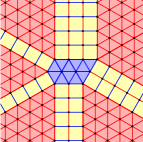
Proposition 9.3 (Fellow traveling in radial flats).

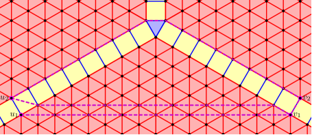
There exist a radial flat plane $F$ such that for every $k>0$ we can find pairs of Gersten-Short geodesics $\alpha$ and $\beta$ in $F$ that start and end an edge apart but where the subspace distance between $\alpha$ and $\beta$ is larger than $k$. In particular, there are radial flat planes in which the Gersten-Short geodesics do not synchronously $k$-fellow travel for any value of $k$.

Proof.

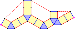
Let $F$ be the radial flat plane shown in Figure 10 with only one bounded region consisting of a single triangle and all other regions unbounded. Next, let $u_{1}$ and $u_{2}$ be two vertices connected by an edge in the interior of one of the three square regions distance $\ell$ from the bounded region. Similarly let $v_{1}$ and $v_{2}$ be two vertices connected by an edge in the interior of a different square region distance $\ell$ from the one bounded region with subscripts chosen so that $u_{1}$ and $v_{1}$ belonging to the boundary of the same triangular region. The figure illustrates such a configuration for $\ell=8$. The Gersten-Short geodesics in the intervals $F[u_{1},v_{1}]$, in $F[u_{2},v_{1}]$ and in $F[u_{1},v_{2}]$ are all roughly parallel (and, in this illustration, roughly horizontal). In $F[u_{2},v_{2}]$, however, the only geodesic, and therefore the unique Gersten-Short geodesic, is an edge path that travels along the boundaries of the square regions and includes an edge from the central triangle. By chosing $\ell$ sufficiently large, the subspace distance between any Gersten-Short geodesic in $F[u_{1},v_{1}]$ and the Gersten-Short geodesic in $F[u_{2},v_{2}]$ can be made as large as possible. In particular, the Gersten-Short geodesics in $F$ do not synchronously $k$-fellow travel for any value of $k$. ∎

At this point it is important to emphasize what this example does and does not show. Although it demonstrates that there are problems that need to be avoided, it does not in and of itself show that Gersten-Short geodesics cannot be used to establish the main conjecture, Conjecture 1.2. This is because the radial flat used as a counterexample is intrinsically aperiodic (Proposition 8.10) and it is not at all clear that such a flat can occur in the universal cover of a compact nonpositively curved triangle-square complex $K$. In fact, we conjecture that no such embeddings exist.

Conjecture 9.4 (Intrinsically aperiodic flats).

If $K$ is a compact nonpositively curved triangle-square complex and $F$ is an intrinsically aperiodic flat then $F$ does not embed into $\widetilde{K}$ and it does not immerse into $K$.

On the other hand, since arbitrarily large portions of this example can occur in potentially periodic flats, this example does show that it is not possible to establish a global value $k_{0}$ such that pairs of Gersten-Short geodesics that start and end within one unit of each other in the universal cover of any compact nonpositively curved triangle-square complex $K$ sychronously $k_{0}$-fellow travel. This is in contrast with the pure cases studied by Gersten and Short where such a global value does indeed exist.

10. Geodesics in periodic flats

At this point we have shown that Gersten-Short geodesics are well-behaved in pure flats and striped flats but they need not fellow travel in radial flats. More over, we have conjectured (Conjecture 9.4) that the only flats that occur in the universal cover of a compact nonpositively curved triangle-square complex are ones that are potentially periodic. In this section we prove that Gersten-Short geodesics are well-behaved in every potentially periodic flat $F$ by extending the earlier results for pure flats and striped flats to flats that are thoroughly crumpled (Proposition 8.10). The argument is of necessity more delicate since the fellow traveling constant $k$ must now vary depending on the fine structure of the flat $F$ under consideration. We begin by imposing order on the wide variety of triangle-square flats in a slightly surprising fashion. In particular, we prove that every triangle-square flat embeds in a single $4$-dimensional PE complex, the product $\mathcal{E}\times\mathcal{E}$ of two Eisenstein planes. This is a tiling of $\mathbb{R}^{4}$ by $4$-polytopes that are the metric product of two equilateral triangles.

Definition 10.1 (Projections).

Let $F$ be a triangle-square flat arranged so that it is colored (Definition 8.5) and imagine altering the metric on $F$ as follows. Let every red edge have length $s$, let every blue edge length $t$ and keep all of the angles the same. Under this new metric the red and blue triangles are rescaled equilateral triangles and the yellow squares become $s$ by $t$ rectangles. For every choice of positive reals $s$ and $t$ the resulting metric space remains a flat, i.e. isometric to $\mathbb{R}^{2}$. Next, consider the limiting case where $s$ shrinks to $0$ while $t$ is fixed at $1$. The end result is (a subcomplex of) the Eisenstein tiling $\mathcal{E}$ and it is the same as the quotient of $F$ that collapses red edges and red triangles to points, and collapses every yellow square to a blue edge. Visually, what happens is that the blue triangles in $F$ slide together. See Figure 11. Similarly, reversing the roles the colors play slides the red triangles together to produce a second projection from $F$ to (a rotated version of) an Eisenstein tiling $\mathcal{E}$. We call these projections $p_{b}:F\longrightarrow\mathcal{E}$ and $p_{r}:F\longrightarrow\mathcal{E}$ where the subscript indicates the color of the edges that survive. Although there are minor ambiguities in the definition of these maps (such as which vertex is sent to the origin and which edges have horizontal images), they are not substantial since any two possible definitions of $p_{b}$ or $p_{r}$ differ by a cellular isometry $\mathcal{E}\to\mathcal{E}$.

Figure 11. A periodic flat with its “red” and “blue” triangles shown on either side.

Locally it is clear that adjacent vertices are identified under one of these projections iff the edge connecting them is one of those that collapses and two sides of a $2$-cell are identified iff they are opposite sides of a square and of the non-collapsing color. The following proposition is the global version of these observations.

Proposition 10.2 (Identifications).

Let $F$ be a colored triangle-square flat and let $p_{r}$ and $p_{b}$ be the red and blue projections defined above. If $u$ and $v$ are vertices of $F$, then $p_{r}(u)=p_{r}(v)$ iff there is a pure blue path in $F$ from $u$ to $v$ and $p_{b}(u)=p_{b}(v)$ iff there is a pure red path in $F$ from $u$ to $v$. More generally, the preimage of vertex in $\mathcal{E}$ is a (possibly degenerate) triangular region and the preimage of an edge is a (possibly degenerate) strip of squares.

As a corollary we note that crumpled plane projections are onto.

Corollary 10.3 (Projections onto $\mathcal{E}$).

If $F$ is a colored crumpled triangle-square flat then the projections $p_{r}$ and $p_{b}$ are onto maps.

Proof.

Let $e$ be an edge in the image of $F$ under one of the projection maps. By Proposition 10.2 its preimage is a strip of squares and because $F$ is crumpled, this strip is finite. The triangles on either end of this strip show that $e$ is in the interior of the image of $F$. Thus the image has no boundary edges and must therefore be all of $\mathcal{E}$. ∎

A more precise statement would be that both projections are onto iff every square region of $F$ is bounded. We are now ready to show that every triangle-square flat, no matter how complicated, can be embedded in a direct product of two Eisenstein planes.

Theorem 10.4 (Embedding flats into $\mathcal{E}\times\mathcal{E}$).

Let $F$ be a colored triangle-square flat and let $p_{b}$ and $p_{r}$ be the blue and red projections defined above. If $p:F\to\mathcal{E}\times\mathcal{E}$ is the map sending $x$ to the ordered pair $(p_{b}(x),p_{r}(x))$, then $p$ is a piecewise linear cellular map that embeds $F$ into the $2$-skeleton of the $4$-dimensional complex $\mathcal{E}\times\mathcal{E}$ built out of copies of the $4$-polytope formed as a direct product of two equilateral triangles.

Proof.

It is easy to check that vertices, edges, triangles and squares in $F$ are sent to vertices, edges, triangles and squares in $\mathcal{E}\times\mathcal{E}$. Thus the only assertion that needs to be verified is that $p$ is an embedding. In fact, it is sufficient to show that $p$ is injective on the vertices of $F$. By Proposition 10.2, if $u$ and $v$ are distinct vertices of $F$ with $p_{r}(u)=p_{r}(v)$, then there is a combinatorial path in $F$ connecting them that consists solely of blue edges. But this blue path remains rigid and unchanged under the projection $p_{b}$. In other words, when $p(u)$ and $p(v)$ agree in the second coordinate, their first coordinates disagree. Repeating this argument with the colors reversed shows that distinct vertices are sent to vertices that might agree on one coordinate but cannot agree on both. ∎

In fact, the embedding of $F$ into $\mathcal{E}\times\mathcal{E}$ satisfies an even stronger condition of being an isometric embedding with respect to the $1$-skeleton metric. Although true for arbitrary flats, we restrict our attention to flats that are crumpled.

Theorem 10.5 (Embedding flats isometrically).

If $F$ be a colored crumpled triangle-square flat and $p:F\to\mathcal{E}\times\mathcal{E}$ is the embedding described above, then $p$ preserves combinatorial distances between vertices. In particular, $p$ isometrically embeds the $1$-skeleton of $F$ into the $1$-skeleton of $\mathcal{E}\times\mathcal{E}$.

Proof.

Because $p$ is a cellular map, the distance between vertices in $F$ is at least as large as the distance between their images in $\mathcal{E}\times\mathcal{E}$. Thus, if the theorem fails, there is a geodesic $\alpha$ in $F$ whose image is not a geodesic in $\mathcal{E}\times\mathcal{E}$ and thus not a geodesic under one of the projection maps. Arguing by contradiction, let $\alpha$ a minimal such path and assume, without loss of generality, that its image is not geodesic under the projection $p_{b}$. The only possibilities are that $p_{b}(\alpha)$ is the old path of a trivial move or it looks like the old path in a doubly-based diagram similar to the one shown on the right in Figure 12, i.e. one that can be shortened using a sequence of triangle-triangle moves followed by a triangle move, (and this includes the old path of triangle move as a degenerate case). That these are the only two possibilities is a relatively straightforward consequence of applying Theorem 5.9 to paths in $\mathcal{E}$. When the image is the old path of a trivial move, the preimage of the edge traversed is a finite strip of squares in $F$ and $\alpha$ traverses three sides of this rectangle. The remaining side shows that $\alpha$ was not a geodesic in $F$, contradiction. When the projection of $\alpha$ looks like the old path of the diagram on the right in Figure 12 we consider the preimage of the diagram $D$ bounded by $p_{b}(\alpha)$ and the straight line geodesic path that connects its two endpoints. For concreteness, assume that this geodesic is horizontal. By Corollary 10.3 the projection $p_{b}$ is onto and by Propostion 10.2 the preimage contains a portion that looks like the diagram on the left in Figure 12 (i.e. triangles connected by finite strips of squares). Since the path $\beta$ along the bottom of this diagram consists solely of edges that are either horizontal or an angle of $\frac{\pi}{6}$ from horizontal, its projections are geodesics which implies that it is sent to a geodesic in $\mathcal{E}\times\mathcal{E}$ and thus a geodesic in $F$. Moreover, $\beta$ is strictly shorter than $\alpha$, since its $p_{b}$ projection is strictly shorter and its $p_{r}$ projection is a geodesic. But this means that $\alpha$ is not a geodesic in $F$, contradiction. ∎

Figure 12. The diagram on the right is a doubly-based disc diagram whose old path can be shortened using two triangle-triangle moves and one triangle move. The diagram on the left shows a portion of a possible preimage of this diagram in a triangle-square flat $F$ with respect to the projection map $p_{b}$. The dashed red lines represent paths in the missing red triangular regions.

By Theorem 10.4 geodesics in the image of a flat correspond exactly with geodesics in the domain, making the following corollary immediate.

Corollary 10.6 (Images of intervals).

Let $F$ be a colored crumpled triangle-square flat and let $p$ be its embedding into $K=\mathcal{E}\times\mathcal{E}$. For all vertices $u$ and $v$ in $F$ with images $u^{\prime}$ and $v^{\prime}$ in $K$, the image of the interval $F[u,v]$ is the intersection of the interval $K[u^{\prime},v^{\prime}]$ with the embedded flat $p(F)$.

This corollary is interesting, at least in part, because intervals in $\mathcal{E}\times\mathcal{E}$ are extremely simple in form.

Proposition 10.7 (Intervals in $\mathcal{E}\times\mathcal{E}$).

For all vertices $u$ and $v$ in the $4$-complex $K=\mathcal{E}\times\mathcal{E}$, the interval $K[u,v]$ is a (possibly degenerate) $4$-dimensional parallelepiped.

Proof.

Because $K$ is a direct product, a vertex $w$ is between $u$ and $v$ iff the image of $w$ is between the images of $u$ and $v$ under both projections $p_{r}$ and $p_{b}$. In particular, the interval in $K$ is a direct product of two intervals in $\mathcal{E}$ and these are (possibly degenerate) $2$-dimensional parallelograms. ∎

With these tools in hand, we now shift our attention to flats that are potentially periodic. The self-similarity of the potentially perioidic flat means that its image under the embedding described above looks, roughly speaking, like an affine plane in $\mathbb{R}^{4}$, a description that can be made precise using the notion of a quasi-isometry.

Definition 10.8 (Quasi-isometries).

Let $f:X\to Y$ be a function between metric spaces. If there are constants $\lambda$ and $\delta$ such that for all $x,x^{\prime}\in X$ with images $y,y^{\prime}\in Y$ both $d_{Y}(y,y^{\prime})\leq\lambda\cdot d_{X}(x,x^{\prime})+\delta$ and $d_{X}(x,x^{\prime})\leq\lambda\cdot d_{Y}(y,y^{\prime})+\delta$, then $f$ is called a quasi-isometric embedding of $X$ into $Y$. If $f$ is also quasi-onto (i.e. there is a constant $c$ such that the $c$-neighborhood of $f(X)$ is all of $Y$) then $f$ is called a quasi-isometry and $X$ and $Y$ are quasi-isometric.

Although it is not immediately obvious from this definition, the relation of being quasi-isometric in an equivalence relation on metric spaces.

Proposition 10.9 (Quasi-flats).

Let $F$ be a colored triangle-square flat and let $p:F\to\mathcal{E}\times\mathcal{E}$ be the corresponding embedding. If $F$ is potentially periodic then its image $p(F)$ is quasi-isometric to a flat affine plane in $\mathbb{R}^{4}\cong\mathcal{E}\times\mathcal{E}$.

Proof.

Let $u$ be a vertex of $F$ embedded in $\mathcal{E}\times\mathcal{E}\cong\mathbb{R}^{4}$. Because $F$ is potentially periodic there are a pair of linearly independent translations from $F$ to itself that generate a cocompact action of $\mathbb{Z}\times\mathbb{Z}$ on $F$. Let $v$ and $w$ be the images of $u$ under these two maps. Since the translations acting on $F$ do not change colors or orientations, they also induce translations of $\mathcal{E}\times\mathcal{E}$ that preserve the image of $F$. In particular, if we let $A$ be the affine span in $\mathbb{R}^{4}=\mathcal{E}\times\mathcal{E}$ of the points $p(u)$, $p(v)$ and $p(w)$, then each point of $p(F)$ lies within a bounded distance of a point in $A$ (since each point $F$ lies within a bounded distance of a point in the orbit of $u$ under the $\mathbb{Z}\times\mathbb{Z}$ action). Thus, by choosing $c$ large enough, $p(F)$ lies in a $c$-neighborhood of $A$ which implies that $F$ is quasi-isometric to $A$. Finally, note that $p(u)$, $p(v)$ and $p(w)$ cannot be collinear since Euclidean planes and lines are not quasi-isometric. Thus $A$ is a $2$-dimensional affine plane. ∎

And finally, in order to understand the behavior of Gersten-Short geodesic in crumpled triangle-square flats, we need to know that the direction of the next choke point can be determined locally.

Lemma 10.10 (Determining the first move).

Let $F$ be a colored crumpled triangle-square flat, let $p$ be the corresponding embedding of $F$ into $K=\mathcal{E}\times\mathcal{E}$ and let $u$ and $v$ be vertices in $F$ with images $u^{\prime}$ and $v^{\prime}$ in $K$. The first move of a Gersten-Short geodesic from $u$ to $v$ is completely determined by the vertex neighborhood of $u$. More specifically, the edges touching $u$ whose images lie in the parallelopiped $K[u^{\prime},v^{\prime}]$ span the initial cell of the first move.

Proof.

By Theorem 7.3 the first move is determined by its first cell which in turn is determined by the edges leaving $u$ that extend to geodesics connecting $u$ to $v$ and such edges are characterized by whether or not their images lie in $K[u^{\prime},v^{\prime}]$. More specifically, if an edge leaving $u$ is the first edge of a geodesic from $u$ to $v$ then by Corollary 10.6 its image lies in $K[u^{\prime},v^{\prime}]$. Conversely, any edge leaving $u$ whose image lies in $K[u^{\prime},v^{\prime}]$ is contained in $K[u^{\prime},v^{\prime}]\cap p(F)$, by Corollary 10.6 it is contained in $p(F[u,v])$, and thus it extends to a geodesic from $u$ to $v$. ∎

As a consequence of local determination of the next move, we can show that Gersten-Short geodesics in a flat do not cross in the following sense.

Corollary 10.11 (Noncrossing geodesics).

Let $F$ be a colored crumpled triangle-square flat and let $p$ be the corresponding embedding of $F$ into $K=\mathcal{E}\times\mathcal{E}$. If $u$ and $v$ are vertices in $F$ with images $u^{\prime}$ and $v^{\prime}$ in $K$, then for every pair of vertices $x$ and $y$ within $1$ unit of $u$ and $v$ in $F$, the next choke point in the Gersten-Short geodesic from $x$ to $y$ is locally determined by the neighborhood of $x$ and the straight line segment from $x$ to this next choke point in $F$ does not cross the straight line segment from $u$ to its next choke point.

Proof.

Since the parallelepipeds $K[u^{\prime},v^{\prime}]$ and $K[x^{\prime},y^{\prime}]$ are nearly identical, except in situations where one of them is degenerate, we can assume by Lemma 10.10 that $v=y$. Next, note that the edges crossed by the straight line segment from $u$ to its first choke point are edges with both endpoints the same distance from $v$ and also note that no other edges in the move have this property. Because $v=y$ the edges crossed by the straight line segment from $x$ to its next choke point have the same property. In particular, neither straight line segment can cross into the interior of the move containing the other. The argument in the exceptional case is essentially the same. ∎

Combining Lemma 10.10 and Corollary 10.11, we now show that image of a Gersten-Short geodesic in $\mathcal{E}\times\mathcal{E}$ is approximately linear until the situation degenerates.

Lemma 10.12 (Roughly linear).

Let $F$ be a colored potentially periodic flat, let $p$ be the corresponding embedding of $F$ into $K=\mathcal{E}\times\mathcal{E}$, and let $u$ and $v$ be vertices in $F$ with images $u^{\prime}$ and $v^{\prime}$ in $K$. There exists a direction vector and a constant depending only on the structure of $F$ and the directions of the sides of the parallelepiped $K[u^{\prime},v^{\prime}]$ so that image under $p$ of any Gersten-Short geodesic from $u$ to $v$ stays with this constant of the line through $u^{\prime}$ with this direction until that point $w^{\prime}$ at which the interval $K[w^{\prime},v^{\prime}]$ degenerates into a lower dimensional parallelepiped.

Proof.

The basic idea goes as follows. Pick $u$ and $v$ so that $K[u^{\prime},v^{\prime}]$ is far from degenerate (i.e. all four side lengths are large). By Lemma 10.10 the first choke point only depends on the neighborhood of $u$ and the directions of the sides of $K[u^{\prime},v^{\prime}]$. Repeat. If the initial side lengths were large enough, then we pass through two vertices that lies in the same $\mathbb{Z}\times\mathbb{Z}$ orbit before the remaining interval is able to degenerate. The vector connecting these two vertices is the vector mentioned in the theorem. By Lemma 10.10 again, the same sequence of moves is now repeated until that point at which the interval remaining degenerates. This shows that this portion of the Gersten-Short geodesic approximates a line in $K$ to within a specified constant. Finally, if we pick any other vertex $x$ close to $u$ and repeat the argument above, we find that the Gersten-Short geodesic from $x$ also has an image in $K$ that approximates a straight line. Because Gersten-Short geodesics in $F$ do not cross (Corollary 10.11) the direction of this line must agree with the previous direction (since it can be bounded on both sides by lines originating in $u$ and other nearby vertices in the same $\mathbb{Z}\times\mathbb{Z}$ orbit as $u$. ∎

Combining these results produces our final main result.

Theorem 10.13 (Fellow traveling in periodic flats).

If $F$ is a potentially periodic triangle-square flat, then there is a value $k$ such that pairs of Gersten-Short geodesics in $F$ that start and end within $1$ unit synchronously $k$-fellow travel.

Proof.

Since this result has already been established from pure and striped flats (Propositions 9.1 and 9.2), we only need to consider flats that are thoroughly crumpled (Proposition 8.10). So assume that $F$ is a potentially periodic thoroughly crumpled triangle-square flat that has been colored with corresponding embedding $p$ into $K=\mathcal{E}\times\mathcal{E}$. Let $\alpha$ and $\beta$ are Gersten-Short geodesics in $F$ that start and end within $1$ unit of each other. We show that they synchronously $k$-fellow travel by showing that they both approximate a pair line segments in the same two directions. By Lemma 10.12, so long as the corresponding intervals in $K$ are not degenerate parallelopipeds, the images of $\alpha$ and $\beta$ approximate straight lines in the same direction. Moreover, once the intervals do degenerate, the remaining portion must approximate the intersection of the affine plane $A$ approximating $p(F)$ (Proposition 10.9) and the affine space containing the degenerate parallelopiped. Because the projection maps from thoroughly crumpled planes are onto (Corollary 10.3), the intersection of these two affine spaces is at most one-dimensional. Combining the constant governing how closely Gersten-Short geodesics travel along a straight line in the non-degenerate portion with the constant governing how closely $p(F)$ approximates $A$, yields a global constant $k$ that is, by construction, independent of $\alpha$ and $\beta$ and only dependent on the periodic structure of $F$ itself. ∎

11. Establishing biautomaticity

In this final section we outline a sequence of steps which, if carried out, would fully establish that a compact nonpositively curved triangle-square complex $K$ has a biautomatic fundamental group (Conjecture 1.2). According to Theorem 3.8, in order to establish the biautomaticity of $\pi_{1}(K)$, one needs to find a collection of paths and then to prove that they fellow travel and form a regular language. We firmly believe that the Gersten-Short geodesics defined have satisfy these conditions. Next, since triangle-square complexes with no immersed flats are already known to be biautomatic (Theorem 8.2), it is natural to focus attention on the flats that do exist. A good first step would be to establish Conjecture 9.4 in order to rule out the existence of intrinsically aperiodic flat planes focusing attention on those potentially periodic flats that immerse into $K$. For each individual potentially periodic flat plane we have shown that there is a value $k$, depending on the flat, so the Gersten-Short geodesics contained in the flat that start and end within $1$ unit of each other synchronously $k$-fellow travel (Theorem 10.13). The natural next step would be to prove the following:

Conjecture 11.1 (Thoroughly crumpled planes).

For any compact nonpositively curved triangle-square complex $K$ there are only finitely many distinct thoroughly crumpled planes that immerse into $K$. As a consequence, there is a global value $k$ depending only on $K$ so that Gersten-Short paths in any flat inside $\widetilde{K}$ that start and end within $1$ unit of each other synchronously $k$-fellow travel.

Once this point has been reached, one should use the fellow traveling constants within planes and the $\textsc{CAT}(0)$ nature of $\widetilde{K}$ overall to prove that all Gersten-Short paths in $\widetilde{K}$ synchronously $k$-fellow travel for some uniform global $k$. Since the constants in pure square, pure triangle and striped flats are small, and periodic crumpled flats have bounded intersection with other flats, this seems reasonable. The necessary arguments might be similar to those used by Chris Hruska in [9]. Finally, once it is known that these paths fellow travel in $\widetilde{K}$, the falsification by fellow traveler property [11] should be invoked to establish the regularity of the language they describe.

References

- [1] B. H. Bowditch. Notes on locally spaces. In Geometric group theory (Columbus, OH, 1992), volume 3 of Ohio State Univ. Math. Res. Inst. Publ., pages 1–48. de Gruyter, Berlin, 1995.
- [2] Tom Brady and Jon McCammond. Braids, posets and orthoschemes. Preprint available at arXiv:0909.4778v1 [math.GR].
- [3] Martin R. Bridson. Geodesics and curvature in metric simplicial complexes. In Group theory from a geometrical viewpoint (Trieste, 1990), pages 373–463. World Sci. Publishing, River Edge, NJ, 1991.
- [4] Martin R. Bridson and André Haefliger. Metric spaces of non-positive curvature, volume 319 of Grundlehren der Mathematischen Wissenschaften [Fundamental Principles of Mathematical Sciences]. Springer-Verlag, Berlin, 1999.
- [5] Murray Elder. Automaticity, almost convexity and falsification by fellow traveler properties of some finitely generated groups. PhD Dissertation, 2000.
- [6] David B. A. Epstein, James W. Cannon, Derek F. Holt, Silvio V. F. Levy, Michael S. Paterson, and William P. Thurston. Word processing in groups. Jones and Bartlett Publishers, Boston, MA, 1992.
- [7] S. M. Gersten and H. B. Short. Small cancellation theory and automatic groups. Invent. Math., 102(2):305–334, 1990.
- [8] Allen Hatcher. Algebraic topology. Cambridge University Press, Cambridge, 2002.
- [9] G. Christopher Hruska. Geometric invariants of spaces with isolated flats. Topology, 44(2):441–458, 2005.
- [10] Jonathan P. McCammond and Daniel T. Wise. Fans and ladders in small cancellation theory. Proc. London Math. Soc. (3), 84(3):599–644, 2002.
- [11] Walter D. Neumann and Michael Shapiro. Automatic structures, rational growth, and geometrically finite hyperbolic groups. Invent. Math., 120(2):259–287, 1995.
- [12] Jacek Świȧtkowski. Regular path systems and (bi)automatic groups. Geom. Dedicata, 118:23–48, 2006.
- [13] B. T. Williams. Two topics in geometric group theory. PhD thesis, University of Southampton, 1998.