Determination of the running coupling constant $\alpha_{s}$ for $N_{f}=2+1$ QCD with the Schrödinger functional scheme

Abstract:

We present an evaluation of the running coupling constant and the quark mass renormalization factor for $N_{f}=2+1$ QCD. The Schrödinger functional scheme is used as the intermediate scheme to carry out non-perturbative running from the low energy region, where physical input is introduced, to deep in the high energy perturbative region, where conversion to the ${\overline{\rm MS}}$ scheme is safely performed.

For numerical simulations we adopted Iwasaki gauge action and non-perturbatively improved Wilson fermion action with the clover term. Seven renormalization scales are used to cover from low to high energy region and three lattice spacings to take the continuum limit at each scale.

Physical inputs are introduced from the previous $N_{f}=2+1$ simulation of the CP-PACS/JL-QCD collaboration, which covered the up-down quark mass range heavier than $m_{\pi}\sim 500$ MeV, and that of PACS-CS collaboration for much lighter quark masses down to $m_{\pi}=155$ MeV.

1 Introduction

The strong coupling constant and quark masses constitute the fundamental parameters of the Standard Model. It is an important task of lattice QCD to determine these parameters using inputs at low energy scales such as hadron masses, meson decay constants and quark potential quantities. The results can be compared with independent determinations from high energy experiments.

In the course of evaluating these fundamental parameters we need the process of renormalization in some scheme. The ${\overline{\rm MS}}$ scheme is one of the most popular schemes, and hence one would like to evaluate these parameters through input of low energy quantities on the lattice and convert it to the ${\overline{\rm MS}}$ scheme. A difficulty in this process is that the conversion is given only in a perturbative expansion, and should be performed at high energy scales much larger than the QCD scale. At the same time the renormalization scale $\mu$ should be kept much less than the lattice spacing to reduce lattice artifacts, namely we require $\Lambda_{\rm QCD}\ll\mu\ll{1}/{a}$. A practical difficulty of satisfying these inequalities in numerical simulations is called the window problem.

The Schrödinger functional (SF) scheme [1, 2, 3, 4, 5] is designed to resolve the window problem. It has an advantage that systematic errors can be unambiguously controlled. A unique renormalization scale is introduced through the box size $L$. A wide range of renormalization scales can be covered by the step scaling function (SSF) technique. The SF scheme has been applied for evaluation of the QCD coupling and the quark mass renormalization factor for $N_{f}=0$ [2, 3] and $N_{f}=2$ [4, 5].

At low energy scales of $\mu\sim 500$ MeV, where physical input is given, we expect the strange quark contribution to be important in addition to those of the up and down quarks. Thus the aim of this proceeding is to go one step further and evaluate the strong coupling constant and the quark mass renormalization factor in $N_{f}=2+1$ QCD. For setting the physical scale we employ two recent large-scale $N_{f}=2+1$ lattice QCD simulations employing non-perturbatively O(a) improved Wilson quark action [6, 7].

Our goal is to evaluate the running coupling constant $\alpha_{s}(M_{Z})$ and the renormalization group invariant (RGI) quark mass $M$. The evaluation of $\alpha_{s}(M_{Z})$ has been performed in Ref. [8], where one finds detailed explanation. The objective for the quark mass is to derive a renormalization factor $Z_{M}(g_{0})$, which converts the bare PCAC mass at bare coupling $g_{0}$ to the RGI mass. The derivation proceed in the same steps as Ref. [3, 5], which we omit in this proceeding.

2 Step scaling function

We adopt the renormalization group improved gauge action of Iwasaki and the improved Wilson fermion action with clover term, whose improvement coefficient $c_{\rm SW}$ is given non-perturbatively [8]. The twisted periodic boundary condition is set for the fermion field in the three spatial directions with $\theta={\pi}/{5}$ for the coupling constant and $\theta=0.5$ for the pseudo scalar density. We adopted two different SF boundary conditions when evaluating the coupling constant [2, 4] and for the pseudo scalar density renormalization factor [3, 5].

We adopt seven renormalized coupling values to cover weak to strong coupling regions. For each coupling we use three boxes $L/a=4,6,8$ to take the continuum limit. For three lattice sizes the values of $\beta$ and $\kappa$ are tuned to reproduce the same renormalized coupling keeping the PCAC mass to zero. On these parameters we evaluate the coupling constant $\overline{g}^{2}(L)$, $\overline{g}^{2}(2L)$ and the renormalization factor ${Z_{P}(g_{0},L/a)}$, ${Z_{P}(g_{0},2L/a)}$. Tiny deviations in the renormalized coupling $\overline{g}^{2}(L)$ and the PCAC mass are corrected perturbatively [9] and we have the SSF’s on the lattice.

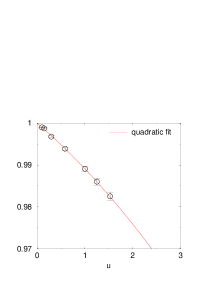
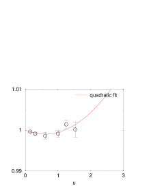
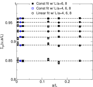
We perform a perturbative improvement of the SSF before taking the continuum limit, for which we need an evaluation of the lattice artifact $\delta_{(P)}(u,a/L)={(\Sigma_{(P)}\left(u,{a}/{L}\right)-\sigma_{(P)}(u))}/{\sigma_{(P)}(u)}$. Although $\delta(u,a/L)$ is evaluated at one loop level its value is rather large and is shown to be applicable only for very weak coupling region [8], which reveals importance of two loop coefficient. On the other hand $\delta_{P}$ is not known for our setup. Instead of calculating $\delta_{P}$ and $\delta$ at one/two-loop level perturbatively we calculate SSF’s directly by Monte-Carlo sampling at very weak coupling $\beta\geq 10$. We define $\delta_{(P)}(u,a/L)$ by a deviation from the perturbative SSF’s $\sigma_{(P)}^{(3)}$ at three (two) loops order [9]. The deviation is fitted in a polynomial form for each $a/L$,

$$1+\delta_{(P)}(u,a/L)=1+d_{1}^{(P)}(a/L)u+d_{2}^{(P)}(a/L)u^{2}.$$ (2.1)

We tried a quadratic fit using data at $u\leq 1.524$, which is plotted in Fig. 1.

Figure 1: Polynomial fit of discrepancy $\Sigma\left(u,{a}/{L}\right)/\sigma^{(3)}(u)$ (upper three figures) and $\Sigma_{P}\left(u,{a}/{L}\right)/\sigma_{P}^{(3)}(u)$ (lower) at high $\beta\gtrsim 4$. The fit is given for each lattice spacings $a/L=1/4$ (left), $a/L=1/6$ (middle) and $a/L=1/8$ (right). Black dotted line is a perturbative one loop behavior and red solid line is a quadratic fit.

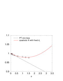
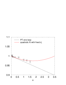
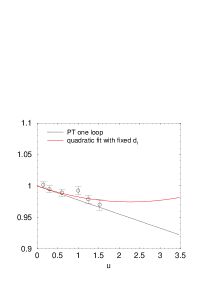
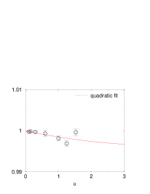
The one loop coefficient $d_{1}(a/L)$ is fixed to its perturbative value for the coupling SSF.

Since the quadratic fit provides a reasonable description of data we opt to cancel the $O(a)$ contribution dividing out the SSF by the quadratic fit. On the other hand the deviation is consistent with zero within one standard deviation for $\delta_{P}(u,1/8)$ at $u\gtrsim 1$ we do not apply an improvement for this case.

Scaling behavior of the improved SSF is plotted in Fig. 2 for the coupling constant and in Fig. 3 for the pseudo scalar density.

Figure 2: The SSF of the coupling constant with its continuum extrapolation at each renormalization scale (left). Right panel is a RG flow of the SSF. Dotted line is three loops perturbative running. Solid line is a polynomial fit.

Figure 3: The SSF for the pseudo scalar density (left). RG flow of the SSF (right).

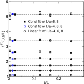
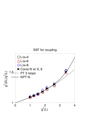
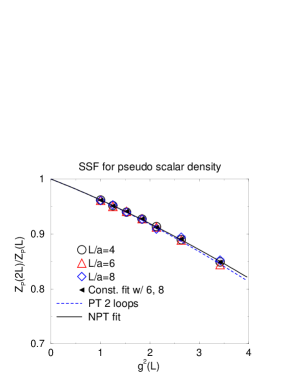
Almost no scaling violation is found. We performed three types of continuum extrapolation: a constant extrapolation with the finest two (filled symbols) or all three data points (open symbols), or a linear extrapolation with all three data points (open circles), which are consistent with each other. We employed the constant fit with these two data point to find our continuum value. The RG running of the continuum SSF is plotted in the same figure at right panel. The fitting functions

$$\sigma(u) = u+s_{0}u^{2}+s_{1}u^{3}+s_{2}u^{4}+s_{3}u^{5}+s_{4}u^{6},$$ (2.2)

$$s_{2} = 0.002265,\quad s_{3}=-0.00158,\quad s_{4}=0.000516,$$ (2.3)

$$\sigma_{P}(u) = 1+p_{0}u+p_{1}u^{2}+p_{2}u^{3},$$ (2.4)

$$p_{1} = -0.002861\quad p_{2}=0.000093.$$ (2.5)

are also plotted (solid line) together with the three/two loops perturbative running (dashed line), where $s_{0}$, $s_{1}$ and $p_{0}$ are set to their perturbative values.

3 Introduction of physical scale

CP-PACS and JLQCD Collaborations jointly performed an $N_{f}=2+1$ simulation with the $O(a)$ improved Wilson action and the Iwasaki gauge action [6]. Three values of $\beta$, $1.83$, $1.90$ and $2.05$ were adopted to take the continuum limit and the up-down quark mass covered a rather heavy region corresponding to $m_{\pi}/m_{\rho}=0.63-0.78$. This project has been taken over by the PACS-CS Collaboration aiming at simulations at the physical light quark masses [7], where results at a single lattice spacing $\beta=1.90$ is available with very light quark masses down to $m_{\pi}/m_{\rho}\approx 0.2$.

We adopt those results to introduce the physical scale into the present work through the low energy reference scale $L_{\rm max}$ in MeV units. We employ the hadron masses $m_{\pi}$, $m_{K}$, $m_{\Omega}$ as inputs and use the lattice spacing $a$ as an intermediate scale.

We evaluate the renormalized coupling and the pseudo scalar density renormalization factor at the same $\beta$ in the chiral limit. The reference scale $L_{\rm max}$ is given by the box size we adopt in this evaluation. The renormalized coupling $\overline{g}^{2}(L_{\rm max})$ should not exceed our maximal value $5.13$ of the SSF very much. The values of the coupling constant and the renormalization factor $Z_{P}(L_{\rm max})$ are listed in Table 1.

$\beta$	$\kappa$	$L_{\rm max}/a$	$\overline{g}^{2}(L_{\rm max})$	$Z_{P}(L_{\rm max})$
$1.83$	$0.13608455$	$4$	$5.565(54)$	$0.57519(32)$
$1.90$	$0.1355968$	$4$	$4.695(23)$	$0.60784(27)$
$2.05$	$0.1359925$	$6$	$4.740(79)$	$0.56641(44)$

Table 1: The renormalized coupling and the renormalization factor $Z_{P}$ at $\beta=1.83$, $1.90$, $2.05$ to define the reference scale $L_{\rm max}$.

We calculate the axial vector current renormalization factor according to the procedure in Ref. [10, 11]. We adopt the renormalization condition [11], which is applicable to non-vanishing PCAC mass, with connected diagrams only. The physical box size is fixed to approximately same value $L\sim 0.75$ fm. Since we did not find any significant $\theta$ dependence we evaluate the renormalization factors at $\theta=0.5$. Preliminary results are listed in table 2.

$\beta$	$\kappa$	size	$m_{\rm AWT}$	$Z_{V}$	$Z_{A}$
$1.83$	$0.138466$	$6^{3}\times 18$	$-0.0003(19)$	$0.751(26)$	$0.965(23)$
$1.90$	$0.137556$	$8^{3}\times 18$	$0.00150(63)$	$0.7424(63)$	$0.8596(77)$
$2.05$	$0.136116$	$12^{3}\times 30$	$0.00291(38)$	$0.7717(41)$	$0.8117(54)$

Table 2: The (axial) vector current renormalization factor at $\beta=1.83$, $1.90$, $2.05$.

4 Strong coupling constant at $M_{Z}$ and RGI mass renormalization factor

We derive the strong coupling constant $\alpha_{s}(M_{Z})$ and $\Lambda_{\overline{\rm MS}}^{(5)}$ according to the procedure in Ref. [8]. The results are listed in Table 3.

$\beta$	$\alpha_{s}(M_{Z})$	$\Lambda_{\overline{\rm MS}}^{(5)}$ (MeV)	$Z_{M}$	$Z_{m}^{\overline{\rm MS}}(2\ {\rm GeV})$
$1.83$	$0.1208(13)$	$243(17)$	$2.084(55)$	$1.616(41)$
$1.90$	$0.1206(14)$	$240(18)$	$1.870(25)$	$1.446(17)$
$2.05$	$0.1198(16)$	$231(20)$	$1.888(26)$	$1.446(15)$
$1.90$	$0.1225(14)$	$266(20)$	$1.870(25)$	$1.484(18)$

Table 3: The strong coupling $\alpha_{s}(M_{Z})$ and the RGI scale $\Lambda_{\overline{\rm MS}}^{(5)}$ for five flavors. Also listed are preliminary results of $Z_{M}$ for the RGI mass and $Z_{m}^{\overline{\rm MS}}$ in the $\overline{\rm MS}$ scheme. The last row for $\beta=1.90$ is given by an input from Ref. [7].

The error includes the statistical error of the renormalized couplings in addition to the statistical error of the lattice spacing. The experimental errors of $m_{c}$, $m_{b}$ and $M_{Z}$ are also included. Preliminary results of the renormalization factor $Z_{M}$ for the RGI mass are also given in Table 3 together with the mass renormalization factor $Z_{m}^{\overline{\rm MS}}(\beta,\mu=2\ {\rm GeV})$ in the $\overline{\rm MS}$ scheme.

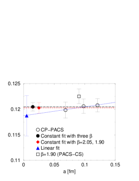
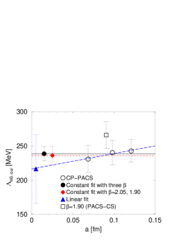
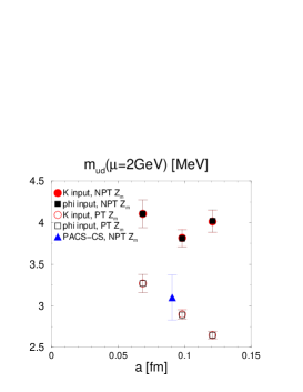
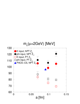
As the last step we take the continuum limit using the three lattice spacings from Ref. [6]. The scaling behavior of $\alpha_{s}(M_{Z})$ and $\Lambda_{\overline{\rm MS}}^{(5)}$ is plotted in Fig. 4 together with that from latest input [7]. Two results agree with each other at the same $\beta=1.90$. We tested three types of continuum extrapolation, which agree with each other and we adopt the constant fit with three data points for our final results:

$$\alpha_{s}(M_{Z})=0.12047(81)(48)(^{+0}_{-173}),\quad\Lambda_{\overline{\rm MS}}^{(5)}=239(10)(6)(^{+0}_{-22})\;{\rm MeV},$$ (4.1)

where the first parenthesis is statistical error and the second is systematic error of perturbative matching of different flavors. The last parenthesis is a difference between the constant and a linear extrapolation and is a systematic error due to finite lattice spacing for physical inputs.

The results from the physical inputs of our latest Ref. [7] are given by

$$\alpha_{s}(M_{Z})=0.1225(14)(5),\quad\Lambda_{\overline{\rm MS}}^{(5)}=266(20)(7)\;{\rm MeV}.$$ (4.2)

Difference between the two physical inputs may reflect mainly a systematic error due to chiral extrapolation toward light quark masses, with the assumption the scaling violation is small also in the latter case.

We also plot preliminary scaling behavior of the light quark masses renormalized at $\mu=2$ GeV in $\overline{\rm MS}$ scheme together with perturbatively renormalized masses [6].

Figure 4: Scaling behavior of $\alpha_{\overline{\rm MS}}(M_{Z})$ (upper left) and $\Lambda_{\overline{\rm MS}}^{(5)}$ (upper right). Scaling behavior of $m_{ud}^{\overline{\rm MS}}$ (lower left) and $m_{s}^{\overline{\rm MS}}$ (lower right); filled circles and squares are from [6], filled triangle is from [12], open symbols are perturbatively renormalized masses [6].

5 Conclusion

We have presented a calculation of the running coupling constant and the quark mass renormalization factor for the $N_{f}=2+1$ QCD in the mass independent Schrödinger functional scheme in the chiral limit. With the “perturbative” improvement the SSF’s shows good scaling behavior and the continuum limit seems to be taken safely with a constant extrapolation of the finest two lattice spacings.

With the non-perturbative renormalization group flow we are able to estimate $\alpha_{s}(M_{Z})$ and the quark mass renormalization factor with some physical inputs for energy scale. The physical scale is introduced from the recent spectrum simulations [6, 7] through the hadron masses $m_{\pi}$, $m_{K}$, $m_{\Omega}$. Our coupling constant (4.1) in the continuum limit is consistent with recent lattice results and the Particle Data Group average $\alpha_{s}(M_{Z})=0.1176(20)$.

References

- [1] M. Lüscher, R. Narayanan, P. Weisz and U. Wolff, Nucl. Phys. B 384 (1992) 168.
- [2] M. Lüscher, R. Sommer, P. Weisz and U. Wolff, Nucl. Phys. B 413 (1994) 481.
- [3] S. Capitani, M. Lüscher, R. Sommer and H. Wittig [ALPHA Collaboration], Nucl. Phys. B 544 (1999) 669.
- [4] M. Della Morte, R. Frezzotti, J. Heitger, J. Rolf, R. Sommer and U. Wolff [ALPHA Collaboration], Nucl. Phys. B 713 (2005) 378.
- [5] M. Della Morte, R. Hoffmann, F. Knechtli, J. Rolf, R. Sommer, I. Wetzorke and U. Wolff [ALPHA Collaboration], Nucl. Phys. B 729 (2005) 117.
- [6] T. Ishikawa et al. [JLQCD Collaboration], Phys. Rev. D 78 (2008) 011502.
- [7] S. Aoki et al. [PACS-CS Collaboration], Phys. Rev. D 79 (2009) 034503.
- [8] S. Aoki et al. [PACS-CS Collaboration], arXiv:0906.3906 [hep-lat].
- [9] A. Bode, P. Weisz and U. Wolff [ALPHA collaboration], Nucl. Phys. B 576 (2000) 517 [Erratum-ibid. B 600 (2001 ERRATA,B608,481.2001) 453].
- [10] M. Lüscher, S. Sint, R. Sommer and H. Wittig, Nucl. Phys. B 491 (1997) 344.
- [11] M. Della Morte, R. Hoffmann, F. Knechtli, R. Sommer and U. Wolff, JHEP 0507 (2005) 007.
- [12] Y. Kuramashi [PACS-CS Collaboration], in this proceeding.