Antiferromagnetic Ising model in scale-free networks
Abstract
The antiferromagnetic Ising model in uncorrelated scale-free networks has been studied by means of Monte Carlo simulations. These networks are characterized by a connectivity (or degree) distribution . The disorder present in these complex networks frustrates the antiferromagnetic spin ordering, giving rise to a spin-glass (SG) phase at low temperature. The paramagnetic-SG transition temperature has been studied as a function of the parameter and the minimum degree present in the networks. is found to increase when the exponent is reduced, in line with a larger frustration caused by the presence of nodes with higher degree.
pacs:
64.60.De, 05.50.+q, 75.10.Nr, 89.75.HcI Introduction
Several types of natural and artificial systems have a network structure, where nodes represent typical system units and edges play the role of interactions between connected pairs of units. This kind of description of complex systems as networks or graphs has attracted much interest in recent years. Thus, complex networks have been used to model various types of real-life systems (biological, social, economic, technological), and to study several processes taking place on them Albert and Barabási (2002); Newman (2003); Newman et al. (2006); Dorogovtsev and Mendes (2003); da F. Costa et al. (2007). Some models of networks have been designed to explain empirical data in various fields. This is the case of the so-called small-world Watts and Strogatz (1998) and scale-free networks Barabási and Albert (1999), which incorporate different aspects of real systems.
In scale-free (SF) networks the degree distribution , where is the number of links connected to a node, has a power-law decay Dorogovtsev and Mendes (2002); Goh et al. (2002). This kind of networks have been found in the internet Siganos et al. (2003), in the world-wide web Albert et al. (1999), for protein interactions Jeong et al. (2001), and in social systems Newman (2001). The origin of such power-law degree distributions was addressed by Barabási and Albert Barabási and Albert (1999), who found that two ingredients are sufficient to explain the scale-free character of networks: growth and preferential attachment. They concluded that the combination of these criteria yields non-equilibrium SF networks with an exponent . One can also consider equilibrium SF networks, defined as statistical ensembles of random networks with a given degree distribution Dorogovtsev and Mendes (2002); Bogacz et al. (2006), for which it is possible to analyze various properties as a function of the exponent .
Cooperative phenomena in complex networks display unusual characteristics due to their peculiar topology Barrat and Weigt (2000); Svenson and Johnston (2002); Herrero (2002); J. Viana Lopes et al. (2004); Candia (2006); Dorogovtsev et al. (2008). In particular, the ferromagnetic (FM) Ising model has been thoroughly studied in scale-free networks Iglói and Turban (2002); Dorogovtsev et al. (2002); Leone et al. (2002); Herrero (2004), and its critical behavior was found to be dependent on the exponent . For finite , a ferromagnetic to paramagnetic transition occurs at a finite temperature . However, when diverges (as happens for ), the spin system remains in an ordered FM phase at any temperature, so that no phase transition appears in the thermodynamic limit.
Here we study the antiferromagnetic (AFM) Ising model in equilibrium (uncorrelated) scale-free networks with several values of the exponent . This model contains the two basic ingredients necessary to produce a spin-glass (SG) phase at low temperature: disorder and frustration. In some spin-glass models, such as the Sherrington-Kirkpatrick model, all spins are assumed to be mutually connected Mydosh (1993); Fischer and Hertz (1991), whereas in others random graphs with finite (low) connectivity are considered Kanter and Sompolinsky (1987); Dean and Lefèvre (2001); Kim et al. (2005); Boettcher (2003). For the AFM Ising model on scale-free networks, we expect to find features intermediate between these two cases.
Spin glasses on complex networks have been studied in recent years by using several techniques, such as transfer matrix analysis Nikoletopoulos et al. (2004), replica symmetry breaking Wemmenhove et al. (2005), defect-wall calculations Weigel and Johnston (2007), and an effective field theory Ostilli and Mendes (2008). In this paper, we employ Monte Carlo (MC) simulations to study the paramagnetic to spin-glass phase transition appearing in scale-free networks. In this line, MC simulations have been carried out earlier to analyze spin-glass phases appearing for the AFM Ising model in Barabási-Albert scale-free networks Bartolozzi et al. (2006), as well as in small-world networks Herrero (2008).
The paper is organized as follows. In Sec. II we describe the networks and the computational method used here. In Sec. III we present results for the heat capacity, energy, and spin correlation, as derived from MC simulations. In Sec. IV we characterize the spin-glass phase through the overlap parameter and transition temperature. The paper closes with the conclusions in Sec. V.
II Model and method
We consider SF networks with degree distribution . They are characterized, apart from the exponent and the system size , by the minimum degree . We assume that for . Our networks are uncorrelated, in the sense that degrees of nearest neighbors are statistically independent. This means that the distribution of degrees of nearest-neighbor nodes fulfills the relation Dorogovtsev and Mendes (2003)
| (1) |
Alternatively, one can use a correlation coefficient defined as
| (2) |
where the averages are taken over all links and is the variance of the degree distribution. This coefficient is zero for uncorrelated networks.
For the numerical simulations we have generated networks with several values of , , and . To generate a network, we first define the number of nodes with degree , according to the distribution , which can be conveniently done by using the so-called transformation method Newman (2005). Then, we ascribe a degree to each node according to the set , and finally connect at random ends of links (giving a total of connections), with the conditions: (i) no two nodes can have more than one bond connecting them, and (ii) no node can be connected by a link to itself. We have checked that networks generated in this way are uncorrelated, i.e. they fulfill Eq. (1), and . The networks considered here contain a single component, i.e. any node in a network can be reached from any other node by traveling through a finite number of links.
Given a network with a particular set of links, we consider an Ising model with the Hamiltonian:
| (3) |
where (), and the coupling matrix is given by
| (4) |
This means that each edge in the network represents an AFM interaction between spins on the two linked nodes. Note that, contrary to the usually studied models for spin glasses in which both FM and AFM couplings are present, in our model all couplings are antiferromagnetic (similarly to Refs. Herrero (2008); Krawczyk et al. (2005)).
For a given network, we carried out Monte Carlo simulations at several temperatures, sampling the spin configuration space by the Metropolis update algorithm Binder and Heermann (1997), and using a simulated annealing procedure. Several variables characterizing the spin system have been calculated and averaged for different values of the considered parameters. For each set of parameters (, , ), 1000 network realizations were generated, and the largest networks included 16000 nodes. In the sequel, we will use the notation to indicate a thermal average for a network, and for an average over networks with a given parameter set.
III Thermodynamic variables
We present first results for the heat capacity per site, , as a function of temperature for several values of the exponent . has been derived from the energy fluctuations at a given temperature, by using the expression
| (5) |
where . We have checked that the results obtained in this way coincide within statistical noise with those derived by calculating the heat capacity as the energy derivative . Note that we take the Boltzmann constant .

The temperature dependence of is displayed in Fig. 1 for scale-free networks with various values of between 3 and 10. The data shown correspond to networks including 8000 nodes. For increasing , we observe that the maximum of shifts to lower , and the peak becomes narrower. This narrowing is in line with that observed earlier for the heat capacity in the AFM Ising model on small-world networks, when the disorder is reduced Herrero (2008). In our case of scale-free networks, larger values of the exponent correspond to networks with a higher homogeneity in the node connectivities (less dispersion in the degree distribution), causing a narrower peak in the heat capacity, as shown in Fig. 1. The peak shift to lower temperatures suggests a transition from a paramagnetic to a SG phase at a temperature that decreases as the exponent rises. For increasing , one reduces the presence of nodes with a large degree, which in turn reduces the degree of frustration in the spin distribution (see below).
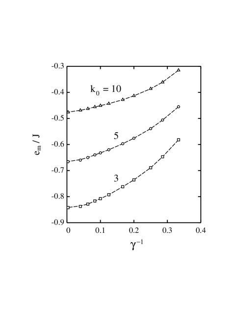
AFM ordering on the considered random networks with power-law distribution of degrees is frustrated by the disorder in the link configuration, and in particular by the presence of loops with an odd number of nodes. The degree of frustration can be quantified by looking at the low-temperature energy of the system, which will be higher for larger frustration. Given the parameters and defining the scale-free networks, we obtain a value for the minimum energy by extrapolating to infinite size the minimum energy reached in our simulations of finite- networks. This extrapolation has been performed by assuming a dependence of the energy on network size of the form:
| (6) |
where is the energy per link for size , is its limit for , and is a fit parameter. This kind of dependence of the low-temperature energy in spin-glass systems was proposed by Boettcher Boettcher (2003), and has been found to be followed by the results of our calculations using the simulated-annealing method. We have checked that our method to obtain a minimum energy for the AFM Ising model on complex networks gives similar results to those found by using extremal optimization Boettcher (2003). In particular, for spin glasses on random graphs with a Poisson distribution of connectivities, we found results very close to those obtained by using this technique Herrero (2008). In any case, the energy found here for each parameter set () will be an upper limit for the lowest energy of the system.
In Fig. 2 we show results for the minimum energy per link found for three values of and several values of the exponent . For a given one observes an increase in as the exponent is reduced. This indicates that the presence of nodes with large degree (hubs), which is favored for small , plays in our context the role of increasing the frustration in the spin arrangement. For a given , one observes also in Fig. 2 an increase in the energy for rising . This shows that an increase in the minimum connectivity (or in the average degree ), causes also a higher frustration in the AFM ordering.
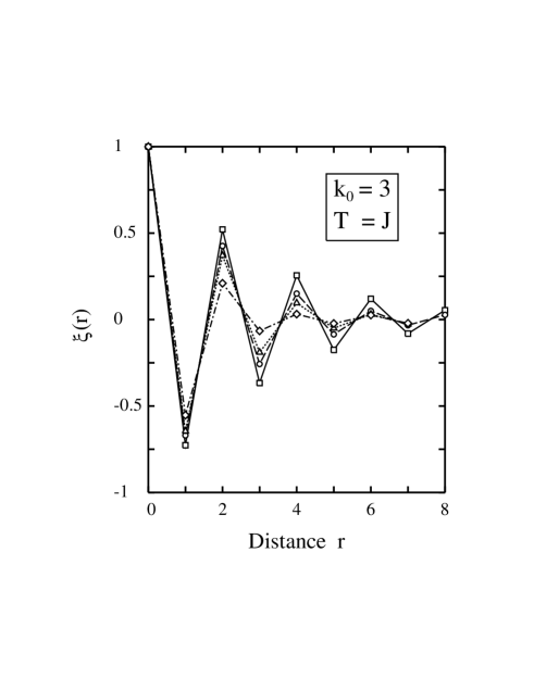
A quantification of the short-range order present in the spin system on scale-free networks can be obtained by calculating the spin correlation
| (7) |
where the subscript indicates that the average is taken for the ensemble of pairs of sites at distance . Note that the dimensionless distance refers to the minimum number of links between two nodes, also called in the literature chemical or topological distance. The correlation is shown in Fig. 3 for several values of the exponent at a temperature . This temperature is below the critical temperature of the paramagnetic-SG transition for all values of (see below). As expected, decreases faster for smaller , due to the presence of nodes with large degree, and consequently a larger frustration of the AFM ordering, as discussed above in connection with the minimum energy per link.
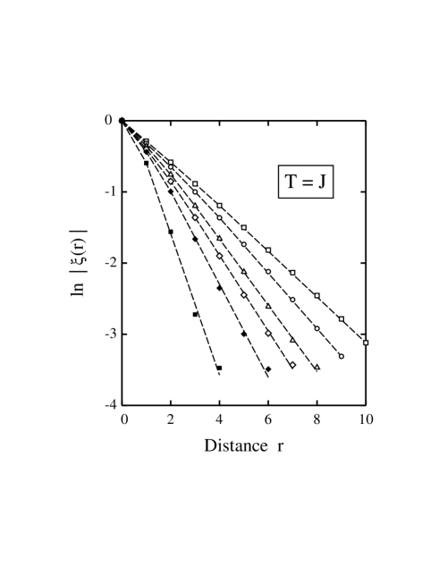
To obtain more direct insight into the reduction of with the distance, we display in Fig. 4 on a semilogarithmic plot for various values. In general, after a short transient for small , one obtains an exponential decrease in the spin correlation with distance, as , being a parameter that depends on temperature as well as on the parameters defining the networks ( and ). For the results shown in Fig. 4, we find a parameter that decreases from 1.01(3) to 0.386(5) when increasing from 3 to 10, and reaches the limit = 0.321(4) for regular random networks with constant degree . We note that here the limit correspond to networks (called regular Bollobás (1998)), in which all nodes have the same degree , and consequently do not include any hub with high degree.
IV Spin-glass behavior
IV.1 Overlap parameter
In the study of spin glasses, it is usual to consider two copies of the same network, with a given realization of the disorder. Then, one considers a spin system on each network, both with different initial values of the spins, and follows their evolution with different random numbers for generating the spin flips Parisi (1983); Kawashima and Young (1996). A particularly relevant parameter is the overlap between the two copies, defined as
| (8) |
where the superscripts (1) and (2) indicate the copies. This parameter is defined in the interval , and the extreme values 1 and –1 correspond to pairs of networks with the same spin configuration (apart from a trivial overall flip in the –1 case).
![[Uncaptioned image]](/html/0908.3560/assets/x5.png)
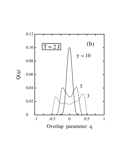
We have calculated the overlap parameter for scale-free networks with various exponents , and derived the probability distribution from Monte Carlo simulations. Results for are presented in Fig. 5. In particular, in Fig. 5(a) we display the distribution of the overlap parameter for networks with at several temperatures. At high temperatures (), the distribution shows a single peak centered at , which is characteristic of a paramagnetic state. This peak has, however, a finite width, which results to be a finite-size effect. It should collapse to a Dirac delta function at in the limit . When the temperature is lowered, broadens around , due to the appearance of an increasing number of frustrated links. At still lower temperatures, frustration is more apparent, and “freezing” of the spins causes the appearance of two peaks in , symmetric respect to , and characteristic of spin-glasses Kawashima and Young (1996); Katzgraber and Young (2002); Bartolozzi et al. (2006); Herrero (2008). Such a distribution is associated to the break of ergodicity occurring in the spin system at low temperatures.
In Fig. 5(b) we show the distribution for three values of the exponent at a fixed temperature . The effect of decreasing for a given is similar to that shown in Fig. 5(a) for lowering the temperature for a given , in the sense that in both cases one passes from a high-temperature paramagnetic phase to a spin-glass with broken ergodicity. From the results displayed in Fig. 5(b), along with those presented in Sect. III (specially Fig. 1 for the heat capacity and Fig. 2 for the minimum energy per link), we expect that the freezing of the spins in the SG phase occurs at lower for larger . In other words, one expects that the transition temperature from paramagnetic to SG will decrease for rising .
IV.2 Transition temperature
The overlap parameter can be further employed to obtain precise values of the paramagnetic-SG transition temperature. To this end, one can use the fourth-order Binder cumulant Binder and Heermann (1997); Kawashima and Young (1996)
| (9) |
which is restricted to the interval [0,1]. On one side, this parameter vanishes at high temperatures, as expected for a Gaussian distribution in a paramagnetic state. On the other side, one has whenever the distribution vanishes everywhere except for , which corresponds to the case of a single ground state, and could be reached at low temperatures. This case () is clearly not expected here due to the onset of frustration, which gives rise to the spin-glass phase.
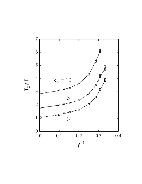
In general increases as temperature is lowered, and the transition temperature can be obtained from the single crossing point for different network sizes Binder and Heermann (1997); Herrero (2008). By employing this method, we have calculated for scale-free networks with several values of the parameters and , and the results obtained are displayed in Fig. 6. In this figure, we have plotted as a function of , and the limit corresponds to regular random networks with . This limit gives a reasonable extrapolation of the values obtained for values up to . For a given minimum degree , the transition temperature increases as is lowered. Also, for a given value of , grows for increasing , similarly to the case of the minimum energy displayed in Fig. 2. We note that the transition temperature derived from the Binder cumulant is in the order of the maximum (negative) temperature derivative of the heat capacity for finite networks, as can be seen by comparing results for in Figs. 1 and 6.
The average degree of scale-free networks can be estimated rather accurately by replacing the sum by an integral. Thus, one finds for networks with and , that the average degree scales as
| (10) |
From this expression, it is clear that and . Since rising or lowering cause an increase in the transition temperature, we observe that in fact a rise in is accompanied by a rise in .
In this context, it is interesting to compare our results for in scale-free networks with those found for the paramagnetic-SG transition in other complex networks. In Ref. Herrero, 2008 it was studied the AFM Ising model on small-world networks generated by rewiring links in a regular lattice Watts and Strogatz (1998). It was found that the transition temperature decreases as the disorder (number of random connections) increases, in networks where the average degree was kept constant (). In the limit of large disorder, those networks approach random networks with a Poisson distribution of degrees, and the transition temperature for the AFM Ising model was found to be . Going back to our random networks with power-law degree distribution, we have an average degree for and [see Eq. (10)]. For these networks, we find , as shown in Fig. 6, a value close to that obtained for small-world-type networks in the large-disorder limit and .
All this could suggest that the transition temperature is proportional to the average degree , irrespective of the details of the networks under consideration. This is, however, not the case, as can be inferred directly from the results displayed in Fig. 6. Looking for example at the data for , we observe that going from to the limit , decreases by a factor of 2 (from 6 to 3). On the other side, is reduced by a factor . Since lowering increases the inhomogeneity in the degree distribution, favoring the presence of nodes with degree much larger than , we find that this inhomogeneity helps to rise the transition temperature.
Bartolozzi et al. Bartolozzi et al. (2006) studied the AFM Ising model on Barabási-Albert scale-free networks, and found a paramagnetic-SG transition temperature . These nonequilibrium networks are characterized by an exponent , and those authors used the particular value of the minimum degree . For these parameters, we find for equilibrium networks a transition temperature , a value somewhat higher than that obtained in Ref. Bartolozzi et al., 2006.
We note that the error bar in the transition temperature grows when is reduced. In fact, the actual value of the cumulant at the crossing point for different values (network sizes) decreases as is lowered, and is near zero for . This coincides with results shown for this cumulant in Ref. Bartolozzi et al., 2006 for Barabási-Albert SF networks, where the value of at the crossing point was less than 0.01. This means that the signal-to-noise ratio in becomes poor, and one has an increasing uncertainty in . For networks with , we could not find a single crossing point for the cumulant corresponding to different network sizes, and a transition temperature cannot be given. We note that these values correspond to SF networks with diverging . In this respect, it is known that the ferromagnetic Ising model in such networks does not show a phase transition, and remains in an ordered FM phase at any temperature in the thermodynamic limit Iglói and Turban (2002); Dorogovtsev et al. (2002); Leone et al. (2002); Herrero (2004). Something similar could happen for the AFM Ising model in these networks. This point remains as a challenge for future research.
V Conclusions
The AFM Ising model in random networks with a power-law distribution of degrees gives rise to a spin-glass phase at low temperature. This is a consequence of the combination of disorder in the networks and frustration caused by the presence of loops with odd number of links. The overlap parameter gives us evidence of this frustration at low temperatures.
The transition temperature from the high-temperature paramagnetic phase to the spin-glass has been studied as a function of the minimum degree and the exponent in the degree distribution. is found to rise for increasing and for lowering .
For a given , both the transition temperature and the minimum energy per link found from our simulations increase as the exponent is lowered. This indicates that the degree of frustration in the spin configurations rises with the presence of nodes with large degree (hubs). The same conclusion can be reached by analyzing the spin correlation as a function of distance, which decays faster for smaller values of .
Acknowledgements.
This work was supported by Ministerio de Ciencia e Innovación (Spain) under Contract No. FIS2006-12117-C04-03.References
- Albert and Barabási (2002) R. Albert and A. L. Barabási, Rev. Mod. Phys. 74, 47 (2002).
- Newman (2003) M. E. J. Newman, SIAM Rev. 45, 167 (2003).
- Newman et al. (2006) M. E. J. Newman, A. L. Barabási, and D. J. Watts, eds., The structure and dynamics of networks (Princeton University, Princeton, 2006).
- Dorogovtsev and Mendes (2003) S. N. Dorogovtsev and J. F. F. Mendes, Evolution of Networks: From Biological Nets to the Internet and WWW (Oxford University, Oxford, 2003).
- da F. Costa et al. (2007) L. da F. Costa, F. A. Rodrigues, G. Travieso, and P. R. Villas Boas, Adv. Phys. 56, 167 (2007).
- Watts and Strogatz (1998) D. J. Watts and S. H. Strogatz, Nature 393, 440 (1998).
- Barabási and Albert (1999) A. L. Barabási and R. Albert, Science 286, 509 (1999).
- Dorogovtsev and Mendes (2002) S. N. Dorogovtsev and J. F. F. Mendes, Adv. Phys. 51, 1079 (2002).
- Goh et al. (2002) K. I. Goh, E. S. Oh, H. Jeong, B. Kahng, and D. Kim, Proc. Natl. Acad. Sci. USA 99, 12583 (2002).
- Siganos et al. (2003) G. Siganos, M. Faloutsos, P. Faloutsos, and C. Faloutsos, IEEE ACM Trans. Netw. 11, 514 (2003).
- Albert et al. (1999) R. Albert, H. Jeong, and A. L. Barabási, Nature 401, 130 (1999).
- Jeong et al. (2001) H. Jeong, S. P. Mason, A. L. Barabási, and Z. N. Oltvai, Nature 411, 41 (2001).
- Newman (2001) M. E. J. Newman, Proc. Natl. Acad. Sci. USA 98, 404 (2001).
- Bogacz et al. (2006) L. Bogacz, Z. Burda, and B. Waclaw, Physica A 366, 587 (2006).
- Barrat and Weigt (2000) A. Barrat and M. Weigt, Eur. Phys. J. B 13, 547 (2000).
- Svenson and Johnston (2002) P. Svenson and D. A. Johnston, Phys. Rev. E 65, 036105 (2002).
- Herrero (2002) C. P. Herrero, Phys. Rev. E 65, 066110 (2002).
- J. Viana Lopes et al. (2004) J. Viana Lopes, Y. G. Pogorelov, J. M. B. Lopes dos Santos, and R. Toral, Phys. Rev. E 70, 026112 (2004).
- Candia (2006) J. Candia, Phys. Rev. E 74, 031101 (2006).
- Dorogovtsev et al. (2008) S. N. Dorogovtsev, A. V. Goltsev, and J. F. F. Mendes, Rev. Mod. Phys. 80, 1275 (2008).
- Iglói and Turban (2002) F. Iglói and L. Turban, Phys. Rev. E 66, 036140 (2002).
- Dorogovtsev et al. (2002) S. N. Dorogovtsev, A. V. Goltsev, and J. F. F. Mendes, Phys. Rev. E 66, 016104 (2002).
- Leone et al. (2002) M. Leone, A. Vázquez, A. Vespignani, and R. Zecchina, Eur. Phys. J. B 28, 191 (2002).
- Herrero (2004) C. P. Herrero, Phys. Rev. E 69, 067109 (2004).
- Mydosh (1993) J. A. Mydosh, Spin Glasses. An Experimental Introduction (Taylor & Francis, London, 1993).
- Fischer and Hertz (1991) K. H. Fischer and J. A. Hertz, Spin Glasses (Cambridge University, Cambridge, 1991).
- Kanter and Sompolinsky (1987) I. Kanter and H. Sompolinsky, Phys. Rev. Lett. 58, 164 (1987).
- Dean and Lefèvre (2001) D. S. Dean and A. Lefèvre, Phys. Rev. Lett. 86, 5639 (2001).
- Kim et al. (2005) D.-H. Kim, G. J. Rodgers, B. Kahng, and D. Kim, Phys. Rev. E 71, 056115 (2005).
- Boettcher (2003) S. Boettcher, Phys. Rev. B 67, 060403(R) (2003).
- Nikoletopoulos et al. (2004) T. Nikoletopoulos, A. C. C. Coolen, I. P. Castillo, N. S. Skantzos, J. P. L. Hatchett, and B. Wemmenhove, J. Phys. A 37, 6455 (2004).
- Wemmenhove et al. (2005) B. Wemmenhove, T. Nikoletopoulos, and J. P. L. Hatchett, J. Stat. Mech.: Theory Exp. p. P11007 (2005).
- Weigel and Johnston (2007) M. Weigel and D. Johnston, Phys. Rev. B 76, 054408 (2007).
- Ostilli and Mendes (2008) M. Ostilli and J. F. F. Mendes, Phys. Rev. E 78, 031102 (2008).
- Bartolozzi et al. (2006) M. Bartolozzi, T. Surungan, D. B. Leinweber, and A. G. Williams, Phys. Rev. B 73, 224419 (2006).
- Herrero (2008) C. P. Herrero, Phys. Rev. E 77, 041102 (2008).
- Newman (2005) M. E. J. Newman, Comtemp. Phys. 46, 323 (2005).
- Krawczyk et al. (2005) M. J. Krawczyk, K. Malarz, B. Kawecka-Magiera, A. Z. Maksymowicz, and K. Kulakowski, Phys. Rev. B 72, 024445 (2005).
- Binder and Heermann (1997) K. Binder and D. Heermann, Monte Carlo Simulation in Statistical Physics (Springer-Verlag, Berlin, 1997).
- Bollobás (1998) B. Bollobás, Modern Graph Theory (Springer-Verlag, New York, 1998).
- Parisi (1983) G. Parisi, Phys. Rev. Lett. 50, 1946 (1983).
- Kawashima and Young (1996) N. Kawashima and A. P. Young, Phys. Rev. B 53, R484 (1996).
- Katzgraber and Young (2002) H. G. Katzgraber and A. P. Young, Phys. Rev. B 65, 214402 (2002).