Coulomb Breakup Reactions
in Complex-Scaled Solutions of the Lippmann-Schwinger Equation

Abstract

We propose a new method to describe three-body breakups of nuclei, in which the Lippmann-Schwinger equation is solved combining with the complex scaling method. The complex-scaled solutions of the Lippmann-Schwinger equation (CSLS) enables us to treat boundary conditions of many-body open channels correctly and to describe a many-body breakup amplitude from the ground state. The Coulomb breakup cross section from the ⁶He ground state into ⁴He+$n$+$n$ three-body decaying states as a function of the total excitation energy is calculated by using CSLS, and the result well reproduces the experimental data. Furthermore, the two-dimensional energy distribution of the $E1$ transition strength is obtained and an importance of the ⁵He($3/2^{-}$) resonance is confirmed. It is shown that CSLS is a promising method to investigate correlations of subsystems in three-body breakup reactions of the weakly-bound nuclei.

1 Introduction

A neutron halo structure is one of the most interesting topics in physics of neutron-rich nuclei. In particular, the two-neutron halo structure observed in the Borromean systems such as ⁶He and ¹¹Li, where any binary subsystem does not have a bound state, has attracted much attention and has been studied by many authors. [1, 2, 3] Theoretically, many works have been performed to understand a binding mechanism of these nuclei based on core+$n$+$n$ three-body models, and an importance of two-neutron correlations has been pointed out. [2, 3, 4, 5, 6, 7] Recently, it has been discussed how to clarify the internal correlations of core-$n$ and $n$-$n$ subsystems in the two-neutron halo nuclei from observables. [8, 9]

Coulomb breakup reactions using a high-$Z$ target such as Pb have been considered as useful tools to investigate the weakly-bound halo nuclei. For ⁶He, the Coulomb breakup cross sections were measured by GSI [11] and MSU [12] groups. For ¹¹Li, there were three sets of data measured at MSU [13], RIKEN [14] and GSI [15], and recently, a new measurement at RIKEN [16] was reported by Nakamura et al. Through those data, we can obtain the understanding not only of ground state properties, but also of breakup reaction mechanisms of halo nuclei. Especially, for two-neutron halo nuclei, the observed cross section is expected to give some important information on internal correlations of core-$n$ and $n$-$n$ subsystems. To understand the correlations of subsystems, it is necessary to investigate the Coulomb breakup reaction based on a reliable theoretical approach.

In our previous studies, we have successfully described the Coulomb breakup reactions of ⁶He and ¹¹Li by using the extended core+$n$+$n$ three-body model and the complex scaling method (CSM). [17, 18, 19] In these analyses, the cross sections were calculated using the response function method (RFM) combined with CSM, which is based on the linear response dominated by the $E1$ strength. For ⁶He, the strength distribution is found to have a peak at around 1 MeV, which is dominated by the transition into the ⁵He(3/2^-)+$n$ two-body continuum states. [17] This result indicates that the sequential breakup process via the ⁵He(3/2^-)+$n$ components is important, and it is shown in Ref. Myo01 that the low energy peak originates from the threshold effect reflecting the halo structure of the ground state. In the ¹¹Li breakup case, it was shown that the non-resonant three-body continuum states of ⁹Li+$n$+$n$ give a comparable contribution with the sequential process via ¹⁰Li+$n$ in the cross section. [19] For both cases, our results well reproduced the observed breakup cross sections with respect to total excitation energies.

In the previous analysis, correlations of subsystems were investigated by separating the transition strength into the components of resonant and non-resonant continuum states. This separation of the strength is useful when we discuss the effects of resonant and non-resonant continuum components on the structure of the strength, and further clarify how much the total strength is exhausted by the individual strength. While the total strength obtained using RMF reproduces the experimental observable, however, the separated strength does not correspond to the observable directly since the experimental data always contains both contributions of resonant and non-resonant continuum states. Then, in this study, we consider another approach, which describes the observables exhibiting the information on internal correlations in a three-body breakup. To extract internal correlations in a three-body system from the observable, it is essential to describe the physical quantities as function of relative energies and momenta in binary subsystems. In fact, experimentally, the breakup cross section was reanalyzed as a function of subsystem energies to understand correlations in two-neutron halo nuclei. [8]

Theoretically, it is a difficult problem to describe physical quantities of three-body breakups with composite particles having internal structures. The standard methods such as the Faddeev, of course, work well when we handle a simple three-body scattering with point particles. However, it is difficult to apply them to the composite particle case. Therefore, an alternative method is needed.

For the two-body case, in Ref. Kr07, it is shown that we can calculate the exact scattering amplitude by using the formal solution of the Lippmann-Schwinger equation (LS Eq.) with the complex-scaled Green’s function even if we handle a scattering problem with composite particles. It is noticed that the Green’s function in Ref. Kr07 is constructed by discretized eigenstates of the complex-scaled Hamiltonian, which are solved in the same manner as bound state cases, and satisfies correct boundary conditions without any explicit enforcement of boundary conditions. Furthermore, it is shown that this complex-scaled Green’s function also works to describe the three-body breakups. [17] It indicates that we can easily apply the procedure in Ref. Kr07 to three-body cases.

Additionally, the formal solution of the LS Eq. is useful to describe physical quantities of three-body breakups as functions of relative energies in subsystems, because it is represented by a solution of an asymptotic Hamiltonian, namely, a plane wave of a three-body system.

The purpose of this work is to extend the theoretical approach in Ref. Kr07 to three-body systems and propose a new method which can evaluate scattering observables as functions of energies in subsystems in three-body breakup reactions. In this paper, we apply this method to the Coulomb breakup reaction of ⁶He and show that this method is capable of investigating internal correlations of subsystems in three-body decaying systems. The reliability of this method is shown by calculating the Coulomb breakup cross section of ⁶He. Furthermore, we evaluate the two-dimensional energy distributions of the $E1$ transition strength associated with the subsystems in ⁶He, which is useful to investigate the internal correlations. In particular, the importance of the ⁵He(3/2^-) resonance in the final states is confirmed.

This paper is organized as follows. In § 2, we give an explanation of our method to describe three-body scattering states as functions of subsystem energies. In § 3, we show the obtained results of the Coulomb breakup reaction of ⁶He, and discuss the reliability of our method and the correlations of subsystems seen in this reaction. The last section, § 4, contains a brief summary.

2 Complex-scaled solution of Lippmann-Schwinger equation
for three-body breakup

In this section, we explain our new method to describe the three-body Coulomb breakup reaction in an energy representation of subsystems. Before describing our method, we give brief explanations of the ⁴He+$n$+$n$ three-body model of ⁶He and CSM in 2.1 and 2.2, respectively. In 2.3, we describe the formalism of our method named as the complex-scaled solutions of the Lippmann-Schwinger equation (CSLS).

2.1 ⁴He+$n$+$n$ model of ⁶He

We first explain the ⁴He+$n$+$n$ three-body model of ⁶He briefly. More detailed explanation is given in Ref. Myo01. In this model, we describe the ⁴He core as the ($0s$)⁴ configuration, whose oscillator length $b_{c}$ is taken as 1.4 fm to reproduce the charge radius of ⁴He. In order to analyze the breakup reactions, it is important to reproduce a threshold energy for each open channel and scattering properties of every subsystem correctly. Hence, we employ the orthogonality condition model (OCM) [21], in which we can use the reliable Hamiltonian whose inter-cluster potentials satisfy the conditions mentioned above.

We solve the following OCM equation for the relative wave function $\chi^{J^{\pi}}$ of the ⁴He+$n$+$n$ system;

$$\hat{H}\chi^{J^{\pi}}(nn)=E\chi^{J^{\pi}}(nn),$$ (1)

where the Hamiltonian for the relative motion is expressed as

$$\hat{H}=\sum_{i=1}^{3}t_{i}-T_{G}+\sum_{i=1}^{2}V_{\alpha n}(\mathbf{r}_{i})+V_{nn}+V^{3}_{\alpha nn}+V_{\text{PF}}.$$ (2)

The operators $t_{i}$ and $T_{G}$ describe a kinetic energy of each cluster and a center-of-mass motion of a three-body system, respectively, and $\mathbf{r}_{i}$ ($i=1$ or $2$) represents a relative coordinate between ⁴He and each valence neutron. The interactions $V_{\alpha n}$ and $V_{nn}$ are given by the microscopic KKNN potential and the effective Minnesota potential, respectively. These potentials well reproduce the scattering data of ⁴He-$n$ and $n$-$n$ systems. In this three-body model, there is a small deficiency of the binding energy ($\sim$ a few hundred keV) of ⁶He ground state, which is considered to come from the ⁴He core polarization effect. [17] In order to improve this deficiency of the binding energy, we employ the effective $\alpha nn$ three-body interaction $V^{3}_{\alpha nn}$ as

$$V^{3}_{\alpha nn}=V_{3}e^{-\nu(\mathbf{r}_{1}^{2}+\mathbf{r}_{2}^{2})},$$ (3)

where $V_{3}=-1.503$ MeV and $\nu=0.07/b_{c}^{2}$ fm^-2.

The component of the Pauli forbidden state is excluded in the relative wave function $\chi^{J^{\pi}}(nn)$ by using the so-called pseudo potential $V_{\text{PF}}$. In the case of ⁶He with the ⁴He core, the Pauli forbidden state $\phi_{\text{PF}}$ for the valence neutrons is the occupied $0s$ state of ⁴He. Then, the pseudo potential $V_{\text{PF}}$ is given as

$$V_{\text{PF}}=\sum_{i=1}^{2}\lambda|\phi^{i}_{\text{PF}}\rangle\langle\phi^{i}_{\text{PF}}|,$$ (4)

where $\lambda$ is taken as $10^{6}$ MeV and $i$ is an index for valence neutrons.

Equation (1) is solved accurately in a few-body technique. We here employ the variational hybrid-TV model, in which the relative wave function of the ⁴He+$n$+$n$ system are expanded on the superposed basis states of the cluster orbital shell model (COSM; V-basis) and the extended cluster model (ECM; T-basis) [22, 17];

$$\chi^{J^{\pi}}(nn)=\chi^{J^{\pi}}_{V}(\boldsymbol{\xi}_{V})+\chi^{J^{\pi}}_{T}(\boldsymbol{\xi}_{T}),$$ (5)

where $\chi^{J^{\pi}}_{V,T}(\boldsymbol{\xi}_{V,T})$ expresses the relative wave function, and $\boldsymbol{\xi}_{V}$ and $\boldsymbol{\xi}_{T}$ are V- and T-type coordinate sets, respectively. The radial component of each relative wave function is expanded by Gaussian basis functions (Gaussian expansion method, GEM). [22, 23] This model successfully describes the observed properties of ⁶He such as the two-neutron binding energy (0.975 MeV) and the matter radius (2.46 fm) of the $0^{+}$ ground state.

2.2 Complex scaling method

In CSM [24, 25, 26], relative coordinates for a many-body system are transformed as

$$U(\theta)\mathbf{r}U^{-1}(\theta)=\mathbf{r}e^{i\theta},$$ (6)

where $U(\theta)$ is a complex scaling operator and $\theta$ is a scaling angle given in a real number. Applying this transformation to the Hamiltonian $\hat{H}$, we obtain the complex-scaled Hamiltonian $\hat{H}^{\theta}$. For $\hat{H}^{\theta}$, the corresponding complex-scaled Schrödinger equation is expressed as

$$\hat{H}^{\theta}\chi^{\theta}=E\chi^{\theta},\ \ \ \ \chi^{\theta}=e^{(3/2)i\theta\cdot f}\chi(\mathbf{r}e^{i\theta}),$$ (7)

where $\chi^{\theta}$ is a complex-scaled wave function. The factor $e^{(3/2)i\theta\cdot f}$ comes from a Jacobian for a volume integral with $f$ degrees of freedom of a system ($f=2$ for a three-body system).

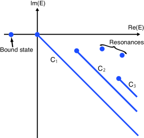
We obtain eigenstates (their biorthogonal states) and energy eigenvalues of the complex-scaled Hamiltonian $\hat{H}^{\theta}$ as $\{\chi^{\theta}_{n}\}$ ($\{\tilde{\chi}^{\theta}_{n}\}$) and $\{E^{\theta}_{n}\}$ with a state index $n$, respectively, by solving the eigenvalue problem of Eq. (7) using a finite number of $L^{2}$ basis functions. In CSM, all energy eigenvalues of unbound states are obtained on the lower half of a complex energy plane, governed by ABC-theorem [24], and their imaginary parts represent outgoing boundary conditions. In ABC-theorem, it is proved that a divergent behavior at an asymptotic region of resonances is transformed to a dumping one by CSM. This condition enables us to obtain many-body resonances by the same calculational way as the bound state case. The resonances are obtained with the complex energy eigenvalues of $E^{\theta}_{n}=E^{r}_{n}-i\Gamma_{n}/2$, where $E^{r}_{n}$ and $\Gamma_{n}$ are resonance energies measured from the threshold and decay widths, respectively, and these energy eigenvalues are independent of the scaling angle $\theta$. On the contrary, energy eigenvalues of continuum states are obtained on the branch cuts of the Riemann sheet, which are rotated down by $2\theta$. This difference of the behaviors between resonances and continuum states makes the energy eigenvalues of resonances isolated from continuum states as shown in Fig. 1. Actually, CSM has been widely employed as a useful tool to identify the resonance of two-, three- and four-body systems. [3, 27]

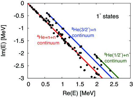
Moreover, CSM is also useful to solve a decay problem of a many-body system. In CSM, the obtained energy eigenvalues of continuum states in a three-body system are classified into two- and three-body ones by ABC-theorem. These continuum states are located on the $2\theta$-rotated branch cuts starting from different thresholds of two- and three-body decay channels, such as ⁵He+$n$ and ⁴He+$n$+$n$ in the case of ⁶He. (See Fig. 1.) The classification of continuum states in CSM imposes that an outgoing boundary condition for each open channel is taken into account by imaginary parts of energy eigenvalues. Using this classification of continuum states, we can describe three-body scattering states without any explicit enforcement of boundary conditions.

Figure 1: Energy spectra of ⁶He in CSM. The left panel is a schematic picture of spectra of the ⁴He+$n$+$n$ system, where the indices $C_{1}$, $C_{2}$ and $C_{3}$ indicate the ⁴He+$n$+$n$, ⁵He(3/2^-)+$n$ and ⁵He(1/2^-)+$n$ continuum spectra, respectively. The right panel is the $1^{-}$ spectra calculated within the present ⁴He+$n$+$n$ model. Three straight lines show the three- and two-body continuum states of ⁴He+$n$+$n$, ⁵He(3/2^-)+$n$ and ⁵He(1/2^-)+$n$ corresponding to $C_{1}$, $C_{2}$ and $C_{3}$, respectively. In the $1^{-}$ spectra calculated with the scaling angle $\theta=27$ degrees, no bound and resonant states are obtained.

2.3 Complex-scaled solutions of the Lippmann-Schwinger equation

We explain a new method of CSLS to describe three-body scattering states, which is capable of calculating physical quantities as functions of subsystem energies in a three-body system.

The formal solution of the Lippmann-Schwinger equation can be described as

$$\Psi^{(\pm)}=\Phi_{0}+\lim_{\varepsilon\to 0}\frac{1}{E-\hat{H}\pm i\varepsilon}\hat{V}\Phi_{0},$$ (8)

where $\Phi_{0}$ is a solution of an asymptotic Hamiltonian $\hat{H}_{0}$. The total Hamiltonian $\hat{H}$ is given in Eq. (2) for ⁶He and the interaction $\hat{V}$ is given by subtracting $\hat{H}_{0}$ from $\hat{H}$. The boundary condition of the scattering state is represented by $\pm\varepsilon$.

When we consider the scattering states of the Borromean system, the asymptotic Hamiltonian $\hat{H}_{0}$ is equivalent to a free Hamiltonian in a three-body system since all the scattering states are described by three-body scattering states and any binary subsystem does not have a bound state. Then, we obtain the following relations:

$$\hat{H}_{0} =\sum_{i=1}^{3}t_{i}-T_{G}$$ (9)

$$\Phi_{0} =\frac{1}{(2\pi^{3})}\exp(i\mathbf{k}\cdot\mathbf{r})\exp(i\mathbf{K}\cdot\mathbf{R}),$$ (10)

where $\mathbf{k}$, $\mathbf{K}$ and $\mathbf{r}$, $\mathbf{R}$ are relative momenta and relative coordinates in a three-body Jacobi coordinate system, respectively. We denote $\Phi_{0}$ by $\langle\mathbf{k},\mathbf{K}|$ and $|\mathbf{k},\mathbf{K}\rangle$ in the bra- and ket-state representation, respectively, to describe the momenta in asymptotic region, $\mathbf{k}$ and $\mathbf{K}$, explicitly.

The formal solution in Eq.(8) for an outgoing three-body scattering state can be rewritten in the ket-state representation as

$$|\Psi^{(+)}(\mathbf{k},\mathbf{K})\rangle=|\mathbf{k},\mathbf{K}\rangle+\lim_{\varepsilon\to 0}\frac{1}{E-\hat{H}+i\varepsilon}\hat{V}|\mathbf{k},\mathbf{K}\rangle,$$ (11)

where the interaction $\hat{V}$ is

$$\hat{V}=\hat{H}-\hat{H}_{0}=\sum_{i=1}^{2}V_{\alpha n}(\mathbf{r}_{i})+V_{nn}+V^{3}_{\alpha nn}+V_{\text{PF}}.$$ (12)

In the present work, we use the complex-scaled Green’s function $\mathcal{G}^{\theta}(E;\boldsymbol{\xi},\boldsymbol{\xi}^{\prime})$. The complex-scaled Green’s function is related to the non-scaled Green’s function $\mathcal{G}(E;\boldsymbol{\xi},\boldsymbol{\xi}^{\prime})$ as

$$\lim_{\varepsilon\to 0}\frac{1}{E-\hat{H}+i\varepsilon}=\mathcal{G}(E;\boldsymbol{\xi},\boldsymbol{\xi}^{\prime})=U^{-1}(\theta)\mathcal{G}^{\theta}(E;\boldsymbol{\xi},\boldsymbol{\xi}^{\prime})U(\theta),$$ (13)

where the complex-scaled Green’s function $\mathcal{G}^{\theta}(E;\boldsymbol{\xi},\boldsymbol{\xi}^{\prime})$ is defined as

$$\mathcal{G}^{\theta}(E;\boldsymbol{\xi},\boldsymbol{\xi}^{\prime})=\left\langle\boldsymbol{\xi}\left|\frac{1}{E-\hat{H}^{\theta}}\right|\boldsymbol{\xi}^{\prime}\right\rangle=\sum_{n}\int\frac{\chi^{\theta}_{n}(\boldsymbol{\xi})\tilde{\chi}^{\theta}_{n}(\boldsymbol{\xi}^{\prime})}{E-E^{\theta}_{n}}.$$ (14)

In derivation of the right hand side of Eq. (14), we use the extended completeness relation (ECR), whose detailed explanation is given in Ref. Myo98 and skipped here. Using this Green’s function constructed by the complex-scaled wave functions of bound, resonant and non-resonant continuum states, we can take into account boundary conditions for all open channels of a three-body system in the form of complex energy eigenvalues $E^{\theta}_{n}$. Then, we can omit the operation of $\varepsilon\to 0$ in the derivation of the complex-scaled Green’s function in Eq. (14). It should be noted that the Green’s function in Eq. (14) is a continuous function with respect to the total energy $E$ while we use discretized energy eigenvalues $E^{\theta}_{n}$ of the complex-scaled Hamiltonian $\hat{H}^{\theta}$. In this calculation, we use 15 Gaussian bases for each relative coordinate, the range of which is taken up to about 20 fm, and the scaling angle $\theta$ is taken as 18 degrees to construct the Green’s function.

Combined with the complex-scaled Green’s function in Eq. (14), the formal solution in Eq. (11) is rewritten as

$$|\Psi^{(+)}(\mathbf{k},\mathbf{K})\rangle=|\mathbf{k},\mathbf{K}\rangle+\sum_{n}\int U^{-1}(\theta)|\chi^{\theta}_{n}\rangle\frac{1}{E-E^{\theta}_{n}}\langle\tilde{\chi}^{\theta}_{n}|U(\theta)\hat{V}|\mathbf{k},\mathbf{K}\rangle.$$ (15)

It is not necessary to apply the complex scaling to the first term of the solution of an asymptotic Hamiltonian. The complex scaling operator $U(\theta)$ in Eq. (15) is processed in the calculation of the matrix elements and does not operate on the complex-scaled eigenstates $\chi^{\theta}_{n}$.

Similarly, let us consider the formal solution for an incoming scattering state. To describe the incoming scattering state, we here consider the bra-state of $\Psi^{(-)}$ with momenta $(\mathbf{k},\mathbf{K})$, which is given as

$$\begin{split}\langle\Psi^{(-)}(\mathbf{k},\mathbf{K})|=&\langle\mathbf{k},\mathbf{K}|\left(1+\lim_{\varepsilon\to 0}\frac{1}{E-\hat{H}-i\varepsilon}\hat{V}\right)^{\dagger}\\ =&\langle\mathbf{k},\mathbf{K}|+\langle\mathbf{k},\mathbf{K}|\hat{V}\lim_{\varepsilon\to 0}\frac{1}{E-\hat{H}+i\varepsilon}.\end{split}$$ (16)

In the derivation of the second line, we assume the hermiticity of $\hat{H}$ and $\hat{V}$. The Green’s function in Eq. (16) is equal to that of Eq. (13), and hence we replce this Green’s function in to the complex-scaled Green’s function. Using Eqs. (13) and (14), we obtain the bra-state of the incoming scattering state as

$$\langle\Psi^{(-)}(\mathbf{k},\mathbf{K})|=\langle\mathbf{k},\mathbf{K}|+\sum_{n}\int\hskip 2.84544pt\langle\mathbf{k},\mathbf{K}|\hat{V}U^{-1}(\theta)|\chi^{\theta}_{n}\rangle\frac{1}{E-E^{\theta}_{n}}\langle\tilde{\chi}^{\theta}_{n}|U(\theta).$$ (17)

Hereafter, we refer Eqs. (15), (17) and their conjugate states as the complex-scaled solutions of Lippmann-Schwinger equation (CSLS).

Additionally, we switch off the pseudo potential $V_{\text{PF}}$ in the calculation of Eqs. (15) and (17) to avoid an instability of numerical results, which comes from the large value of $\lambda=10^{6}$ MeV, while the wave functions $\chi^{\theta}_{n}$ are solved with the pseudo potential. By switching off the pseudo potential, the antisymmetrization in the scattering state is approximately ignored, but it is not a serious problem, since the antisymmetrization in the intermediate states are considered when we solve the eigenstates $\chi^{\theta}_{n}$. In fact, it will be shown in the next section that the obtained result in CSLS shows a reasonable agreement with the previous result in Ref. Myo01 and the calculated breakup cross section well reproduces the trend of the experimental data.

2.4 E1 transition in complex-scaled solutions of the Lippmann-Schwinger equation

To calculate the $E1$ transition strength and the Coulomb breakup cross section, we start with the two-dimensional momentum distribution of the $E\lambda$ transition strength given as

$$\frac{d^{6}B(E\lambda)}{d\mathbf{k}d\mathbf{K}}=\frac{1}{2J_{\text{g.s.}}+1}\left|\langle\Psi^{(-)}(\mathbf{k},\mathbf{K})||\hat{O}(E\lambda)||\Phi_{\text{g.s.}}\rangle\right|^{2},$$ (18)

where $\Phi_{\text{g.s.}}$ is a ground state wave function and $\hat{O}(E\lambda)$ is a transition operator with a rank $\lambda$. $J_{\text{g.s.}}$ is a total spin of the ground state.

Using Eq. (18), we derive an $E\lambda$ transition strength with respect to the total energy $E$ of a system as follows;

$$\frac{dB(E\lambda)}{dE}=\iint d\mathbf{k}d\mathbf{K}\frac{d^{6}B(E\lambda)}{d\mathbf{k}d\mathbf{K}}\delta\left(E-\frac{\hbar^{2}k^{2}}{2\mu}-\frac{\hbar^{2}K^{2}}{2M}\right),$$ (19)

where $\mu$ and $M$ are reduced masses of subsystems corresponding to the two momenta $\mathbf{k}$ and $\mathbf{K}$, respectively. Similarly, we obtained the two-dimensional energy distribution as

$$\frac{d^{2}B(E\lambda)}{d\varepsilon_{1}d\varepsilon_{2}}=\iint d\mathbf{k}d\mathbf{K}\frac{d^{6}B(E\lambda)}{d\mathbf{k}d\mathbf{K}}\delta\left(\varepsilon_{1}-\frac{\hbar^{2}k^{2}}{2\mu}\right)\delta\left(\varepsilon_{2}-\frac{\hbar^{2}K^{2}}{2M}\right),$$ (20)

where $\varepsilon_{1}$ and $\varepsilon_{2}$ are subsystem energies in a three-body system.

In the next section, we shall show the total energy and two-dimensional energy distributions of the $E1$ transition strength, and discuss the correlations of subsystems in the Coulomb breakup of ⁶He.

3 Energy distributions of $E1$ transition strength for ⁶He

We demonstrate that CSLS is useful to investigate internal correlations of subsystems in the final states.

Figure 2: (Color online) Total energy distribution of the $E1$ transition strength of ⁶He. The red and blue curves show the result including FSI and the one of the direct breakup, respectively.

Figure 3: (Color online) The obtained Coulomb breakup cross section measured from the ⁴He+$n$+$n$ threshold energy. The red and blue lines show the original result in CSLS and the folded one with the experimental resolution, respectively. The observed cross section (open square) is taken from Ref. Au99.

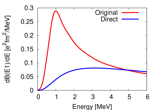
Before discussing the correlations of subsystems in the final states, we first calculate the total energy distributions of the $E1$ transition strength from the ground state of ⁶He into ⁴He+$n$+$n$ three-body scattering states to show the importance of the final state interaction (FSI). Using Eq. (19), we obtain the result of the total energy distribution measured from the ⁴He+$n$+$n$ threshold energy as shown in Fig. 3. From this original result, it is confirmed that the strength possesses a sharp peak at around 1 MeV. In order to recognize FSI, we also calculate the strength without FSI. When we switch off FSI, scattering state of ⁶He can be described only by first term of the right hand side of Eq. (15) since the interaction $\hat{V}$ is zero. Then, the strength without FSI, which is equivalent to the one of the transition from the ground state into non-interacting three-body continuum states, is calculated by taking the first term of Eq. (15). This transition strength of the direct breakup is also shown in Fig. 3. It is found that the direct breakup one has a small strength with a broad bump at around 3 MeV. This large difference between the original and the direct breakup strengths indicates the importance of FSI to explain the low energy enhancement in the $E1$ transition strength of ⁶He. The result of Fig. 3 is consistent with the previous result in Ref. Myo01.

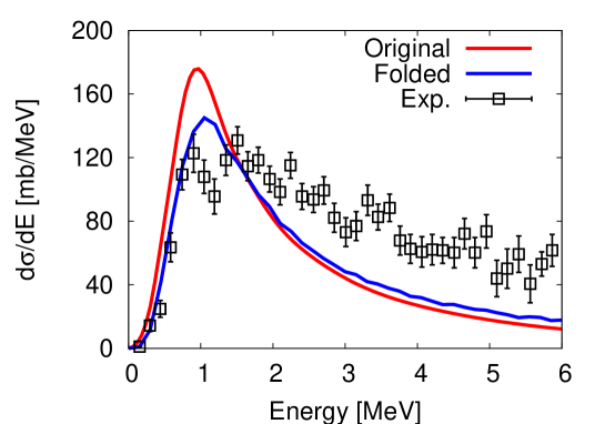
Here, we also show the reliability of our calculation by comparing the obtained result using CSLS and the experimental data. We drive the breakup cross section of ⁶He using the obtained $E1$ transition strength and the equivalent photon method. The experimental data are taken from Ref. Au99. In Fig. 3, two strengths are shown; One is the original result in CSLS and another is the folded one by the experimental resolution [11]. The obtained cross section in CSLS has a peak at around 1 MeV and well reproduces the observed trend. This good agreement of the cross section implies the reliability of CSLS to describe the three-body scattering states since the validity of the three-body model has been already shown in Ref. Myo01.

Figure 4: (Color online) Twi-dimensional energy distribution of the $E1$ transition strength corresponding to the ⁴He-$n$ and ⁵He-$n$ subsystems.

Figure 5: (color online) Two-dimensional energy distribution of the direct breakup as same as Fig. 5.

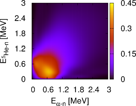
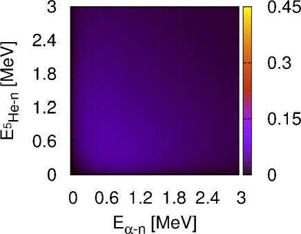
Next, we investigate correlations of subsystems in the final states. Using Eq. (20), we evaluate the two-dimensional energy distribution of the $E1$ transition strength of ⁶He, associated with the ⁵He subsystem. The result is shown in Fig. 5, where $\varepsilon_{1}$ and $\varepsilon_{2}$ in Eq. (20) are the relative energies of ⁴He-$n$ ($E_{\alpha\text{-}n}$) and ⁵He-$n$ ($E_{{}^{5}\text{He-}n}$) systems, respectively. It is clearly seen that the strength is concentrated on around $E_{\alpha\text{-}n}\sim 0.7$ MeV, which agrees with the ⁵He(3/2^-) resonance energy. Hence, the importance of the ⁵He(3/2^-) resonance in the Coulomb breakup reaction of ⁶He is directly shown in the physical observables using CSLS, which is consistent with the previous analysis using RFM. [17] We also show the two-dimensional energy distribution of the direct breakup strength in Fig. 5 to clarify the FSI in the two-dimensional energy distributions. From Fig. 5, we find that no clear peak structure appears without FSI. This result indicates that the correlations in the two-dimensional energy distribution mainly comes from the FSI and the sequential decay via the ⁵He(3/2^-)+$n$ channel is important in the Coulomb breakup reaction of ⁶He.

4 Summary

In the present study, we developed a new approach called the complex-scaled solutions of Lippmann-Schwinger equation (CSLS), which enables us to describe a scattering state for three-body breakups of the Borromean system and to calculate the observables with respect to not only the total energy but also the subsystem energies. Using CSLS, we reproduced the observed Coulomb breakup cross section nicely, and confirmed that the ⁵He(3/2^-) resonance plays an important role in the Coulomb breakup reaction. This CSLS approach makes us to extract the correlations of subsystems from the observables and is useful to study the properties of the weakly-bound nuclei not only for the ground state, but also for the scattering states. The detailed analysis on the subsystems correlations such as ⁴He-$n$ and $n$-$n$ systems in the Coulomb breakup reaction of ⁶He is forthcoming. It is also interesting to perform the analysis of the two-neutron halo nuclei ¹¹Li using this method.

References

- [1] I. Tanihata, J. of Phys. G 22(1996), 157.
- [2] M.V. Zhukov, B.V. Danilin, D.V. Fedorov, J.M. Bang, I.J. Thompson and J.S. Vaagen, Phys. Rep. 231(1993), 151.
- [3] S. Aoyama, T. Myo, K. Katō and K. Ikeda, Prog. Theor. Phys. 116(2006), 1 and references therein.
- [4] Y. Suzuki, Nucl. Phys. A 528(1991), 395.
- [5] H. Esbensen and G.F. Bertsch, Nucl. Phys. A 542(1992), 310.
- [6] S. Funada, H. Kameyama and Y. Sakuragi, Nucl. Phys. A 575(1994), 93.
- [7] K. Hagino and H. Sagawa Phys. Rev. C 72(2005), 044321.
- [8] L.V. Chulkov et al., Nucl. Phys. A 759(2005), 23.
- [9] S.N. Ershov, B.V. Danilin and J.S. Vaagen, Phys. Rev. C 74(2006), 014603.
- [10] T. Nakamura, et. al., Phys. Lett. B 331(1994), 296.
- [11] T. Aumann, et al., Phys. Rev. C 59(1999), 1252.
- [12] J. Wang, et al., Phys. Rev. C 65(2002), 034306.
- [13] K. Ieki, et al., Phys. Rev. Lett. 70(1993), 730.
- [14] S. Shimoura, T. Nakamura, M. Ishihara, N. Inabe, T. Kobayashi, T. Kubo, R.H. Siemssen, I. Tanihata and Y. Watanabe, Phys. Lett. B 348(1995), 29.
- [15] M. Zinser, et. al., Nucl. Phys. A 619(1997), 151.
- [16] T. Nakamura, et al., Phys. Rev. Lett. 96(2006), 252502.
- [17] T. Myo, K. Katō, S. Aoyama and K. Ikeda, Phys. Rev. C 63(2001), 054313.
- [18] T. Myo, S. Aoyama, K. Katō and K. Ikeda, Phys. Lett. B 576(2003), 281.
- [19] T. Myo, K. Katō, H. Toki and K. Ikeda, Phys. Rev. C 76(2007), 024305.
- [20] A.T. Kruppa, R. Suzuki and K. Katō, Phys. Rev. C 75(2007), 044602.
- [21] S. Saito, Prog. Theor. Phys. 40(1968), 893; 41(1969), 705; Prog. Theor. Phys. Suppl. 62(1977), 11.
- [22] S. Aoyama, S. Mukai, K. Katō and K. Ikeda, Prog. Theor. Phys. 93(1995), 99.
- [23] E. Hiyama, Y. Kino and M. Kamimura, Prog. Part. Nucl. Phys. 51(2003), 223.
- [24] J. Aguilar and J.M. Combes, Commun. Math. Phys. 22(1971), 269; E. Balslev and J.M. Combes, Commun. Math. Phys. 22(1971), 280.
- [25] Y.K. Ho, Phys. Rep. 99(1983), 1.
- [26] N. Moiseyev, Phys. Rep. 302(1998), 211.
- [27] T. Myo, K. Katō and K. Ikeda, Phys. Rev. C 76(2007), 054309.
- [28] T. Myo, A. Ohnishi and K. Katō, Prog. Theor. Phys. 99(1998), 801.