On a test of the modified BCS theory performance
in the picket fence model

Abstract

The errors in the arguments, numerical results, and conclusions in the paper “Test of a modified BCS theory performance in the picket fence model” PV by V.Yu. Ponomarev and A.I. Vdovin are pointed out. Its repetitions of already published material are also discussed.

I Introduction

The modified BCS (MBCS) theory and its extension, the modified Hartree-Fock-Bogoliubov (MHFB) theory, have been proposed and developed in a series of papers MBCS1 ; MBCS2 ; MHFB ; MBCS3 ; MBCS4 between 2001 and 2007. The aim of these theories is to restore the unitarity relation $R^{2}=R$ for the generalized single-particle density matrix $R$, which is violated within the conventional BCS and HFB theories at finite temperature $T$. This restoration leads to an application of the secondary Bogoliubov transformation from the conventional quasiparticle operators to the modified quasiparticle ones. As a result the MBCS equation is obtained. The main merit of the MBCS theory is that it is a fully microscopic theory, which shows that the phase transition from the superfluid phase to the normal one (the SN phase transition) is smoothed out in finite systems. The MBCS pairing gap does not collapse at the critical temperature $T_{c}$ of the SN phase transition, where the conventional BCS gap vanishes. It also points out, for the first time, that the origin of the smoothing out of the SN-phase transition is the quasiparticle-number fluctuations (QNF), which are ignored in the conventional BCS and HFB theories. The MBCS theory has been applied with success in several open-shell realistic nuclei MBCS1 ; MBCS2 ; MHFB and tested by its authors in an exactly solvable pairing model with $\Omega$ doubly folded levels MBCS3 ; comment , which is often referred to as the Richardson model, ladder model, or picket-fence model (PFM). Being an approximation that deals with the fluctuations due to the system finiteness, the MBCS theory is sensitive to the size of the system under consideration. Within the half-filled PFM, e.g., i.e. when $N=\Omega$, where $N$ is the number of particles, the MBCS gap decreases smoothly with increasing the temperature $T$ up to a certain temperature $T_{M}$ ($>T_{c}$), where a discontinuity occurs (See Refs. MBCS3 ; MBCS4 and references therein). For a single-particle spectrum with the level distance $\epsilon$ equal to 1 MeV, it has been found that his maximal temperature $T_{M}$ decreases almost linearly with decreasing $T$ from a value as high as $T_{M}\simeq$ 24 MeV for $N=\Omega=$ 100 to a value as low as $T_{M}\simeq$ 0.7 MeV for $N=\Omega=$ 6 MBCS3 . In Ref. comment it has been pointed out, for the first time, that the asymmetry of the QNF with respect to the Fermi energy is the reason that causes the decrease of $T_{M}$ with $N$. In the same Ref. comment , it has also been found that it is sufficient to add just one more level, i.e. $\Omega=N+1$, to restore the symmetry of the QNF up to much higher $T_{M}$. This allows to extend the temperature region of applicability of the MBCS theory to a temperature as high as $T\leq$ 5 - 6 MeV for all values of the particle number $N$ (for $\epsilon=$ 1 MeV and the pairing interaction $G=$ 0.4 MeV). The MBCS theory has been the subject of exchanging criticisms between us comment ; MBCS3 ; MBCS4 and the authors of Refs. PV1 ; PV2 . In a recent paper PV , the same authors reiterated their criticism by repeating the results of the same test within the PFM. Regrettably, beside largely duplicating the contents, which have already been published in Refs. MBCS2 ; MHFB ; MBCS3 ; comment ; MBCS4 ; PV1 ; PV2 , the authors of Ref. PV added nothing new but further serious mistakes and false conclusions. The aim of the present article is to point out the errors as well as the repetitions in Ref. PV , which is referred to hereafter as the test PV .

II Incorrect statements and erroneous results

II.1 Chemical potential

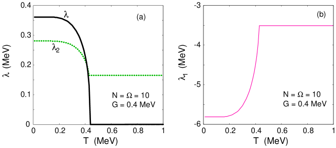
The authors of the test PV claim that the chemical potential of the PFM should not change with temperature $T$, remaining always in the middle of the single-particle spectrum taken to be zero in this case. This statement is true only within the BCS theory for the half-filled case (i.e. $N=\Omega$) if the self-energy correction term $\sim Gv_{j}^{2}$ is neglected in the single-particle energies. Within the BCS theory at $T\neq$ 0, the chemical potential $\lambda$ is determined as a Lagrangian multiplier so that the average particle number within the grand canonical ensemble (GCE) has the correct value. This is because the BCS theory violates the particle number, causing quantal fluctuations of particle number, and ignores the effects due to the QNF at finite temperature as well. In any other theory, including the MBCS theory, where these effects and/or correlations beyond the mean field are partially or fully taken into account, the chemical potential $\lambda$ becomes a function of $T$. An example is the well-known Lipkin-Nogami (LN) method LN , which is an approximate particle-number projection to partially eliminate the particle-number fluctuations in the BCS theory. The LN method yields $\lambda=\lambda_{1}+2\lambda_{2}(N+1)$. These chemical potentials are shown in Fig. 1 as functions of $T$ for the PFM with $N=\Omega=$ 10 and $G=$ 0.4 MeV. So long as the pairing gap $\Delta$ exists, all of them change with $T$, and none of them remains at zero.

Figure 1: (Color online) Chemical potentials $\lambda$, $\lambda_{1}$ and $\lambda_{2}$ as functions of $T$ within the Lipkin-Nogami method for the PFM with $N=\Omega=$ 10 and $G=$ 0.4.

Figure 2: (Color online) Chemical potentials $\mu$ as a functions of $T$ at $G=$ 0.4 MeV (a), and a function of $G$ at $T=$ 0 (b) for the PFM with $\Omega=N+1=$ 11 (a), and $\Omega=N=$ 10 (b). The exact CE results are shown as the solid lines. In (a) the exact CE result for $\Omega=$ 10 is also shown as the thin solid line. The BCS and MBCS results are shown in (a) as the dotted and dashed lines, respectively.

The exact definition of the chemical potential $\mu$ is the difference between the ground-state (internal) energies of the systems with $N\pm 2$ particles Ring , namely

$$\mu_{+}=\frac{1}{2}[{\cal E}(N+2)-{\cal E}(N)]~{},\hskip 14.22636pt\mu_{-}=\frac{1}{2}[{\cal E}(N)-{\cal E}(N-2)]~{},$$ (1)

$$\mu=\frac{1}{2}(\mu_{+}+\mu_{-})=\frac{1}{4}[{\cal E}(N+2)-{\cal E}(N-2)]~{},$$ (2)

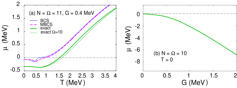
where ${\cal E}(N)$ denotes the ground-state energy of the $N$-particle system in the zero-temperature case, or its internal (total) energy at finite temperature $T$. In the latter case, the thermal average within the GCE is carried out for a system which exchanges its energy and particle number with a heat bath. If the particle number of the system is fixed, the canonical ensemble (CE) should be used for thermal averaging. The PFM is a system with a fixed number of particles, where no particle number fluctuations are possible. Therefore the meaningful exact results should be those obtained within the CE by using the partition function constructed from the exact eigenvalues of the pairing Hamiltonian [See Eqs. (3) for the expressions of the total energies within the GCE and CE]. As shown by the solid lines in Fig. 2, the chemical potential $\mu$ strongly depends on temperature $T$ and the interaction parameter $G$. From Fig. 2 (a) one can also see that the performance of the MBCS theory (the dashed line) is quite reasonable.

Figure 3: (Color online) Entropies as functions of $T$ for $N=\Omega=$ 10 at $G=$ 0.4 MeV. The thermodynamic entropies $S_{th}$ are shown in panels (a), while panels (b) display the quasiparticle entropies $S_{qp}$. In the upper panels, (a1) and (b1), these quantities are shown in the logarithmic scale, whereas the linear scale is used in the lower panels, (a2) and (b2). The notations for the lines are shown in (a1), including the “exact results” of the test PV (circles). In (b1) and (b2) the exact GCE and CE single-particle entropies are also shown as faint thick and thin solid lines, respectively.

II.2 Entropies

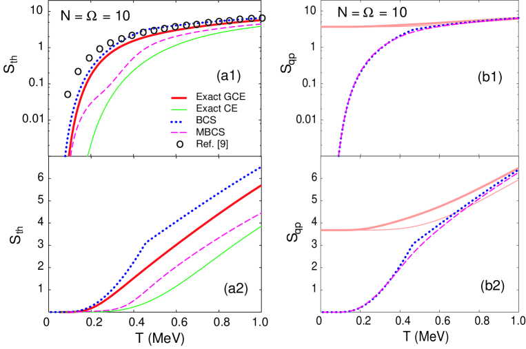
Regarding the entropies, the results that the authors claim as the exact thermodynamic entropy, denoted as circles in Fig. 7 (a) of Ref. PV , are incorrect. The same circles are also shown in Fig. 3 (a1). The correct exact GCE and CE results for this quantity are shown as thick and thin solid lines, respectively, in Fig. 3 (a1) (in the logarithmic scale) and Fig. 3 (a2) (in the linear scale). They are obtained from the same Eq. (17) of the test PV with the total energies calculated within the GCE and CE by using the textbook definitions, namely

$$\langle{\cal E}\rangle_{\rm GCE}=\frac{1}{{\cal Z}(\beta,\lambda)}\sum_{s,n}{\cal E}_{s}^{(n)}e^{\beta\lambda n}p_{s}(\beta,n)~{},\hskip 14.22636pt\langle{\cal E}\rangle_{\rm CE}=\frac{1}{Z(\beta,N)}\sum_{s}{\cal E}_{s}^{(N)}p_{s}(\beta,N)~{},$$ (3)

with the grand partition function ${\cal Z}(\beta,\lambda)$, and partition function $Z(\beta,n)$ defined as

$${\cal Z}(\beta,\lambda)=\sum_{n}e^{\beta\lambda n}Z(\beta,n)~{},\hskip 5.69054pt{Z}(\beta,n)=\sum_{s}p_{s}(\beta,n)~{},\hskip 14.22636ptp_{s}(\beta,n)=d_{s}^{(n)}e^{-\beta{\cal E}_{s}^{(n)}}~{}.$$ (4)

In Eq. (4), ${\cal E}_{s}^{(n)}$ are the eigenvalues of the pairing Hamiltonian for the system with $n$ particles, whereas $d_{s}^{(n)}$ are their degeneracies. The GCE sum in Eq. (3) is carried out over all $n=$ 1, $\ldots$, $\Omega$-1 with blocking properly taken into account for odd $n$. As compared to these exact GCE values [thick solid line in Fig. 3 (a1)], the results of the test PV (circles) at $T\leq$ 0.1 MeV are wrong by more than one order of magnitude. Meanwhile, the thermodynamic entropy obtained within the MBCS theory (the dashed lines) are found sandwiched between the exact GCE and CE results. The quasiparticle entropy obtained within the MBCS theory agrees quite well with the BCS one, except for the region around the critical temperature $T_{c}$, where the BCS gap collapses. At high $T$ they both converge to the exact GCE result for the single-particle entropy as expected [See faint thick solid lines Figs. 3 (b1) and 3 (b2)]. The exact GCE and CE single-particle entropies are obtained by using the occupation numbers $f_{j}$ on the $j$th single-particle orbital within the GCE and CE, respectively. The latter are the ensemble averages of the exact state-dependent occupation numbers $f_{j}^{(s)}$, namely

$$f_{j}^{(\rm GCE)}=\frac{1}{{\cal Z}(\beta,\lambda)}\sum_{s,n}f_{j}^{(s,n)}z_{s,n}(\beta,\lambda)~{},\hskip 14.22636ptf_{j}^{(\rm CE)}=\frac{1}{{Z}(\beta,N)}\sum_{s}f_{j}^{(s,N)}p_{s}(\beta,N)~{},$$ (5)

with

$$f_{j}^{(s)}=\frac{\sum_{k}N_{j}^{(k)}(C_{k}^{(s)})^{2}}{\sum_{k}(C_{k}^{(s)})^{2}}=\sum_{k}N_{j}^{(k)}(C_{k}^{(s)})^{2}~{},\hskip 5.69054pt{\rm with}\hskip 5.69054pt\sum_{k}(C_{k}^{(s)})^{2}=1~{},$$ (6)

where $(C_{k}^{(s)})^{2}$ determine the weights of the eigenvector components, and $N_{j}^{(k)}$ are the partial occupation numbers weighted over the basis states $|k\rangle$.

III Repetitions of published material

Sections 2 and 3 of the test PV repeat the arguments of Ref. PV2 , where the same authors replied to the our comments in Ref. comment . This is clearly seen, e.g., in Fig. 1 of the test PV , which is obtained by putting all the lines from the upper panels (for the pairing gaps) of Fig. 1 in Ref. PV2 into one panel. The only difference is that Fig. 1 of Ref. PV2 is for N = 10, while the same figure in the test PV is presented for N = 14. This modification obviously offers no new physics as compared to Fig. 1 in the previously published Ref. PV2 .

Section 3 of the test PV also repeats the discussion of Refs. MHFB ; MBCS3 ; MBCS4 ; comment ; PV1 ; PV2 . As we have pointed out in Refs. MHFB ; MBCS3 ; MBCS4 ; comment , the validity of the MBCS depends on how the QNF is taken into account. If the single-particle spectrum is too small, the QNF can be large even at the top and bottom of the spectrum, and its profile becomes strongly asymmetric with respect to the middle of the spectrum already a low $T$. This leads to some artifacts as negative values of the pairing gap, or a discontinuity in its temperature dependence. Therefore, a criterion is introduced to include the QNF symmetrically from both sides of the Fermi energy in such a way that the negative and positive wings discussed in Fig. 2 (b) of Ref. MHFB nearly cancel each other. For the PFM under consideration, it turns out that, for small $N$, e.g. $N\leq$ 14 with the level distance equal to 1 MeV and G= 0.4 MeV, it is sufficient to enlarge the space by just one level $\Omega=N+1$ to achieve a symmetric profile of the QNF up to a rather high temperature, while adding or subtracting more levels again decreases the value of the limiting temperature, at which the QNF profile becomes asymmetric. For realistic heavy nuclei, such as ¹²⁰Sn e.g., this criterion is often unnecessary so long as the whole single-particle space is included (Fig. 1 - f of Ref. MHFB ). In this respect, Figs. 2 - 4 of the test PV and the related discussions therein are just a disguised tautology since they demonstrate nothing but the asymmetry of the QNF, which has already been shown and discussed previously in Fig. 2 of Ref. MBCS3 , and Fig. 1 of Ref. MBCS4 .

In Fig. 2 (b) of our paper MHFB , the partial components of the thermal gap are shown to clarify the temperature dependence of the total gap, which is a physical quantity. It seems that the authors of the test PV misunderstood this idea when they borrowed our results to divide the MBCS thermal gap into the hole and particle gaps [See Eqs. (15) and (16) of the test PV ]. They summed up the values of $\delta\Delta_{j}$ discussed in our paper MHFB over the levels below the Fermi energy separately from those above it, and considered these two sums as the hole and particle gaps, respectively. Obviously, such separation of the thermal gap into the hole and particle gaps as two physical quantities is misleading. The MBCS thermal gap is level-independent, and induced by all the QNF, which should be included by summation over all quasiparticle orbitals. Figures 5 (c) and 5 (d) of the test PV repeat the upper panel of Fig. 3 in Ref. PV1 , which has previously been published by the same authors under almost the same title. Two additional panels (a) and (b) bear no additional physics information. These issues have been refuted by us in Ref. comment .

Last but not least, that the MBCS theory does not cure the particle-number fluctuation (PNF) has already been discussed long ago in Ref. MBCS2 , where the PNF was calculated for several neutron-rich Ni isotopes MBCS2 . This is the reason why several methods of particle-number projection were applied within the MBCS theory in Ref. MBCS4 , whose calculations were carried out not only for the PFM but also for the realistic nucleus ¹²⁰Sn. Therefore, Fig. 6 and the related discussions in the test PV are redundant because they just reiterate a well-known fact by using an oversimplified toy model with just two levels.

IV Introducing misleading quantities and making wrong conclusions

A part from the errors and repetitions mentioned above, the authors of the test PV also introduced misleading discussions by comparing the MBCS predictions of quasiparticle energies with the “exact” ones (See Fig. 3 of the test PV ), whose definition remains completely obscure. A quasiparticle state is an approximation, which arises from the canonical Bogoliubov transformation, and is related to the mean-field concept. So long there is no exact mean field, there cannot be exact quasiparticle energies. The eigenvalues of the PFM, which are obtained by diagonalizing the pairing Hamiltonian or solving the Richardson’s equations, are not quasiparticle energies. In order to have a better agreement with the exact eigenvalues one needs to go beyond the conventional BCS theory to take into account the correlations beyond the mean field. It is for this purpose that the particle-particle self-consistent RPA (SCRPA) ppRPA1 ; ppRPA2 (for low value of the pairing interaction parameter $G$) and quasiparticle RPA (SCQRPA) SCQRPA (for an arbitrary value of $G$) were developed. But while the SCRPA and SCQRPA can describe rather well the low excitation energies, they cannot describe the complicate splitting of high-lying levels due to configuration mixing in the exact solutions Yuz .

Figure 4: (Color online) MBCS gaps $\bar{\Delta}$ as functions of temperature $T$ obtained within the PFM, which has $N=$ 10 particles, and $\Omega=N+k$ levels. (a) Results obtained with $G=$ 0.6 MeV, $k=$ 0, 1,…, 8; (b) Results obtained with $G=$ 0.55 MeV, $k=$ 0, 1, 2, and 3. The numbers at the right margins of (a) and (b) show the corresponding values of $\Omega$. The single-particle energies for the sets (a) and (b) are specified in the text.

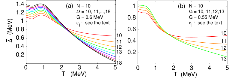
Apart from the conclusions of the test PV , which obviously become invalid as a consequence of the above analysis, the authors of the test PV also claim: “We confirm that there exists a single example of the PFM (with the number of levels $\Omega$ equal to the number of particles $N$ plus one) in which the MBCS produces the thermal behavior of the pairing gap similar to the one of a macroscopic theory up to rather high temperatures. On the other hand, we demonstrate that in all other examples of the PFM with $\Omega\neq N$ the theory predicts phase transitions of unknown types at a much lower temperature.” Of course, this statement is incorrect. It is valid only for a PFM with $N=$ 10, $G=$ 0.4 MeV with the level distance $\epsilon=$ 1 MeV. It is not difficult to find counter examples, some of which are shown in Fig. 4. It depicts the MBCS pairing gaps $\bar{\Delta}$ obtained for the PFM with $N=$ 10, and $\Omega=N+k$, which are grouped in two sets. The set in Fig. 4 (a) consists of nine MBCS gaps, which are obtained with $k=$ 0, …, 8 by using $G=$ 0.6 MeV, and the following single-particle energies: $\epsilon_{j}=2.1\times j$ (MeV) for $j\leq$ 3 and $j\geq$ 7, whereas $\epsilon_{j}=\epsilon_{3}+j-3$ (MeV) for 4$\leq j\leq$ 6. The set in Fig. 4 (b) represents four MBCS gaps, which are obtained with $k=$ 0, 1, 2, and 3 by using $G=$ 0.55 MeV, and the following single-particle energies: $\epsilon_{j}=2.1\times(j-5.5)$ (MeV) for $j\leq$ 3 and 7 $\leq j\leq$ 10, $\epsilon_{j}=j-5.5$ (MeV) for 4 $\leq j\leq$ 6, and $\epsilon_{j}=2.1\times(0.55\times\epsilon_{10}+j-10)$ (MeV) for 11 $\leq j\leq$ 13. All thirteen MBCS gaps in Fig. 4 are smooth functions of $T$ at 0 $\leq T\leq$ 5 MeV. This figure clearly shows how changing the size of the system affects the tail of the gap at $T\geq$ 2 MeV in these cases. These examples and the analysis in the present article are more than sufficient to rule out all the conclusions of the test PV .

V Conclusion

In conclusion, the test PV not only repeats already published results, but also contains incorrect statements and detectable errors, which make its conclusions invalid.