Comparison of Different Pairing Fluctuation Approaches to BCS-BEC Crossover

Abstract

The subject of BCS - Bose Einstein condensation (BEC) crossover is particularly exciting because of its realization in ultracold Fermi gases and its possible relevance to high temperature superconductors. In the paper we review that body of theoretical work on this subject which represents a natural extension of the seminal papers by Leggett and by Nozières and Schmitt-Rink (NSR). The former addressed only the ground state, now known as the “BCS-Leggett” wave-function and the key contributions of the latter pertain to calculations of the superfluid transition temperature $T_{c}$. These two papers have given rise to two main and, importantly, distinct, theoretical schools in the BCS-BEC crossover literature. The first of these extends the BCS-Leggett ground state to finite temperature and the second extends the NSR scheme away from $T_{c}$ both in the superfluid and normal phases. It is now rather widely accepted that these extensions of NSR produce a different ground state than that first introduced by Leggett. This observation provides a central motivation for the present paper which seeks to clarify the distinctions in the two approaches. Our analysis shows how the NSR-based approach views the bosonic contributions more completely but it treats the fermions as “quasi-free”. By contrast, the BCS-Leggett based approach treats the fermionic contributions more completely but it treats the bosons as “quasi-free”. In a related fashion, the NSR based schemes approach the crossover between BCS and BEC by starting from the BEC limit and the BCS-Leggett based scheme approaches this crossover by starting from the BCS limit. Ultimately, one would like to combine these two schemes. There are, however, many difficult problems to surmount in any attempt to bridge the gap in the two theory classes. In this paper we review the strengths and weaknesses of both approaches. The flexibility of the BCS-Leggett phase and its ease of handling make it more widely used in $T=0$ applications, although, the NSR-based schemes are more widely used at $T\neq 0$. To reach a full understanding, it is important in the future to invest effort in investigating in more detail the $T=0$ aspects of NSR-based theory and at the same time the $T\neq 0$ aspects of BCS-Leggett theory.

I Introduction

The subject of BCS-Bose Einstein condensation (BEC) crossover has recently become an extremely active research area. This is due principally to the discovery Greiner et al. (2003); Jochim et al. (2003); Regal et al. (2004); Zwierlein et al. (2004, 2005); Kinast et al. (2004a); Bartenstein et al. (2004a); Kinast et al. (2005); Bourdel et al. (2004); Partridge et al. (2005) of superfluid phases in ultracold Fermi gases which exhibit this crossover. Adding to the importance of this work is the view espoused by a number of theorists Randeria (1995); Chen et al. (2005a); Levin and Chen (2007); Leggett (2006); Perali et al. (2002) that the high temperature superconductors are mid-way between BCS and BEC. Now, with an unambiguous realization of this scenario in the fermionic superfluids, one has the opportunity to investigate this physical picture more closely and, it is hoped, gain insight into the cuprate superconductors. Equally exciting is the opportunity to generalize, and in the process, gain insight into what is arguably the paradigm for all theories in condensed matter physics: Bardeen Cooper Schrieffer theory. For all these reasons a large number of variants of BCS-BEC crossover theory have been suggested in the literature. It is the purpose of the present paper to present an overview of two main classes of theories, discussing their strengths and weaknesses. Contrasting and comparing different approaches will, hopefully, point to new directions for future theoretical and experimental research.

Initial theoretical work Eagles (1969); Leggett (1980) on the subject of BCS-BEC crossover focussed on a ground state which was shown to be the same as that proposed by Bardeen Cooper and Schrieffer, when it is extended to accomodate a continuous evolution from BCS to BEC. We call this the “BCS-Leggett” state. Here the chemical potential is solved self consistently as the attractive interaction strength is varied. In this way it became clear that the BCS trial wavefunction was far more general than was originally thought. Somewhat later, Noziéres and Schmitt-Rink (NSR) Nozières and Schmitt-Rink (1985) presented a scheme for calculating the transition temperatures $T_{c}$, which made the case that the evolution from BCS to BEC was again continuous at finite temperature.

The discovery of high temperature superconductivity and the observation that their coherence length $\xi$ (or pair size) was anomalously small led T. D. Lee and R. Friedberg to argue that one should include bosonic degrees of freedom in addressing high $T_{c}$ superconductors. These authors introduced Friedberg and Lee (1989a, b) the “boson-fermion” model almost immediately after the discovery of cuprate superconductivity. In a similar vein, Randeria and co-workers Randeria (1995) proposed that the NSR scheme might be directly applicable to these exciting new materials. Subsequently other theorists have applied this BCS-BEC crossover scenario to the high $T_{c}$ cuprates Chen et al. (1998a); Micnas and Robaszkiewicz (1998); Ranninger and Robin (1996); Perali et al. (2002). Additional support has come from the experimental condensed matter community among whom a number Uemura (1997); Renner et al. (1998); Deutscher (1999); Junod et al. (1999) have presented data which can be interpreted within this picture. Adding to the enthusiasm is the observation of a ubiquitous (albeit controversial) “pseudogap” phase Lee et al. (2006); Chen et al. (2005a); Levin and Chen (2007) in the underdoped cuprates, which was argued Randeria (1998); Jankó et al. (1997) to be consistent with a BCS-BEC crossover scenario.

The characterization of pseudogap effects associated with BCS-BEC crossover was, in fact, a crucial step. It was first recognized that one should distinguish the pair formation temperature $T^{*}$ from the condensation temperature $T_{c}$ Micnas et al. (1990); Randeria (1995). That the magnetic properties of the normal phase in the temperature regime between $T_{c}$ and $T^{*}$ would be anomalous was pointed out on the basis of numerical calculations, on a two dimensional lattice. Here it was found that the spin susceptibility was depressed at low temperatures Trivedi and Randeria (1995) and this depression was associated with a “spin gap” which is to be distinguished Randeria (1998) from a pseudogap which affects the “charge channel” as well. The fact that BCS-BEC crossover theory was, indeed, associated with a more general form of pseudogap, thus, required further analysis and calculations. Using the formalism of the present paper, subsequent, theoretical studies of the spectral function (both above Jankó et al. (1997) and below Chen et al. (2001) $T_{c}$) and the superfluid density Chen et al. (1998b) showed that a normal state pairing gap appeared in both the spin and charge channels and, furthermore, affected the behavior below $T_{c}$ as well Chen et al. (1998b) as above.

The BCS-BEC crossover approach was applied to the ultracold Fermi gases, by Holland and co-workers Milstein et al. (2002) and by Griffin and Ohashi Ohashi and Griffin (2002) in advance of the discovery of fermionic superfluidity. The two groups predicted that the magnetic field tuneability associated with an atomic Feshbach resonance would lead to an unambiguous realization of the crossover scenario. These earliest applications to ultracold Fermi gases considered a Hamiltonian rather similar to the “boson-fermion” model of Lee and co-workers Friedberg and Lee (1989a, b) where the bosons were related to the so-called closed channel molecules of the Feshbach resonance and the fermions with the open channel. Subsequent work has shown that these two channel complications can be essentially ignored so that the description of Fermi gas superfluidity is addressed using the same, simpler (or one channel) model as was used in the cuprates.

There is now a fairly extensive theoretical literature Chen et al. (2005a); Levin and Chen (2007); Griffin and Ohashi (2003); Pieri et al. (2004a) on the Fermi gas superfluids. Nevertheless, there are two main theoretical schools, which have emerged. These address a wide variety of different issues and experiments. The first of these builds more directly on the BCS-Leggett ground state and its finite temperature extensions Jankó et al. (1997); Kosztin et al. (1998); Chen et al. (1999); Stajic et al. (2004); Kinnunen et al. (2004). The second approach Ohashi and Griffin (2002); Milstein et al. (2002); Perali et al. (2003); Pieri et al. (2004a); Griffin and Ohashi (2003); Pieri and Strinati (2000); Perali et al. (2004a) builds on the contribution of Nozieres and Schmitt Rink which addressed a calculation of the transition temperature $T_{c}$. The NSR scheme has been extended by these and other authors away from $T_{c}$ both in the superfluid and normal phases. It is now rather widely accepted that these extensions of NSR produce a different ground state Chen et al. (2005a); Perali et al. (2004b); Diener et al. (2008) than that first introduced by Leggett Leggett (1980) and by Eagles Eagles (1969). This observation provides a central motivation for the present paper. We want to set down our current understanding of what is known about the NSR-based theories from zero to very high $T$ and similarly, address how the simplest ground state of BCS-Leggett evolves with increasing temperature away from zero. Since the ground states are different, we can safely assume that the finite $T$ behavior is as well. It should be stressed that while we attribute these author group names to the two different schools, the eponymous authors are not the origin of the theory reviewed here. The original paper by Leggett was only concerned with the ground state and that by Nozieres and Schmitt-Rink recapitulated and expanded on the results of Leggett and then went on to compute $T_{c}$ using an approach which was not associated with this same (BCS-Leggett) $T=0$ state.

The task in any finite temperature crossover theory is to arrive at a characterization of the thermal excitations of both the normal and superfluid phases. From this analysis all transport and thermal properties can in principle be obtained. Without any detailed microscopic theory one can still anticipate the general features of BCS-BEC crossover theory. In the BCS regime and below $T_{c}$, the excitations are the usual fermionic quasi-particles with an excitation gap equivalent to the order parameter. This gap represents the energy cost of unbinding the condensate pairs. By contrast, above $T_{c}$ this gap is absent and the normal state is a Fermi liquid. In the BEC regime, it is energetically unfavorable to break up the pairs and so the excitations are purely bosonic above and below $T_{c}$. In the superfluid phase, they are, moreover, gapless. In between, in the interesting unitary regime, the excitations are expected to be a mix of fermionic and bosonic character. Here, importantly even the normal state has some bosonic features associated with the formation of “pre-formed pairs”. These pairs arise from stronger than BCS attractive interactions. As a consequence there is an excitation (pseudo)gap for fermionic excitations which appears above $T_{c}$. With progressively lower temperatures below $T_{c}$, more and more of these pairs drop into the condensate. The challenge then is to treat the strongly interconnected bosonic and fermionic degrees of freedom in the most physically correct fashion.

Below $T_{c}$ the two schools referred to above emphasize different aspects of this picture. One can summarize in the simplest fashion the key differences. The NSR-based approach views the bosonic contributions more completely but it treats the fermions as “quasi-free”. Many body effects are effectively absent in the fermionic dispersion relation (called $E_{\mathbf{k}}^{o}$, which appears in the counterpart gap equation), except via a renormalization of the fermionic chemical potential $\mu^{*}$. The BCS-Leggett based approach treats the fermionic contributions more completely than the alternative approach but it treats the bosons as “quasi-free”. Many body effects in the bosonic dispersion, (which we call $\Omega_{\bf q}^{o}$), are absent in the gap equation except via an effective pair mass renormalization $M^{*}$.

More specifically, the NSR approach incorporates a linear dispersion in the bosonic degrees of freedom at small wavevector which is associated with the collective mode spectrum of the condensate. However, $T_{c}$ is calculated in the same way as for non-interacting fermions, except for the renormalization in $\mu^{*}$. The BCS-Leggett based approach in effect approximates the bosonic degrees of freedom associated with the non-condensed pairs. While the collective modes of the order parameter have a linear dispersion, the non-condensed pairs have a quadratic dispersion and represent otherwise free “bosons”. Here, $T_{c}$ is calculated in the presence of a pseudogap so that the condensing fermionic quasiparticles have admixed bosonic character.

It is reasonable to conclude that the NSR based scheme approaches the crossover between BCS and BEC by starting from the BEC limit and the BCS-Leggett based scheme approaches this crossover by starting from the BCS limit. For the former, indeed, the boson-like propagators which one deduces are found to have many similarities to Bogoliubov theory for true bosons. It is claimed Andrenacci et al. (2003) that the NSR-based approach is most accurate at temperatures low compared to $T_{c}$, presumably because there the bosonic degrees of freedom are those associated with the condensate and its collective modes. Thus, it is reasonable to assume that this represents the better ground state. By contrast the BCS-Leggett based scheme is more suitable at moderate temperatures within the superfluid phase and up to the pairing onset temperature $T^{*}$. Above $T^{*}$, the two approaches can be viewed as equivalent.

Ultimately, one would like to combine these two schemes. There are, however, many difficult problems to surmount in any attempt to bridge the gap in the two theory classes. Not only is it difficult to effect such a combination but, thus far, there is no mean field theory of a weakly interacting Bose gas Shi and Griffin (1998); Andersen (2004) which addresses the entire regime from $T=0$ through and above $T_{c}$ and which does not have at the same time a problematic first order transition. Thus, for the interacting Bose gases, there is no counterpart of BCS theory which works so well over the entire temperature range. These complications, in true Bose systems, appear to be transmitted to NSR based theories of the Fermi gases. These spurious first order transitions fir can lead to derivative discontinuities in the density profiles at the condensate edge and non-monotonic or discontinuous behavior in the superfluid density, even in the intermediate or unitary regime. BCS theory, by contrast, exhibits none of these effects. If one is to find a smooth crossover between BCS and BEC at all temperatures $T$ these issues will need to be overcome.

Additional problems appear if one tries to bridge the gap by starting with the BCS-Leggett based scheme. The first task is to establish how non-condensed pair effects modify the collective mode spectrum. This appears to be a difficult problem. While, some progress has been made Kosztin et al. (2000) towards computing pseudogap effects on the Anderson Bogoliubov mode, there is, however, an even greater difficulty in coupling the non-condensed pairs with the renormalized collective modes. To arrive at this hybridization, one needs to introduce boson-boson coupling which requires that one go beyond the simple T-matrix scheme which one considers in addressing the non-condensed component. This is not to say that the coupling between condensed and non-condensed pairs is absent, it must be there in the ultimate theory, but it will be difficult to implement.

To summarize, the ground state produced by NSR-based approaches is likely to represent an improvement over that of the BCS-Leggett based approach, particularly when it comes to quantitative comparisons, and most particularly when the system is on the BEC side of resonance. However at the semi-quantitative or qualitative level one is often required to consider the BCS-Leggett ground state, and its finite temperature extensions, since globally this state behaves more smoothly. Moreover, this state is easier to handle and can accomodate inhomogeneities via Bogoliubov deGennes theory Machida and Koyama (2005); Chien et al. (2006a); Sensarma et al. (2006); BdG . It is the also the primary way to study phases with population imbalance Sheehy and Radzihovsky (2006); De Silva and Mueller (2006); Chien et al. (2006b); Ric ; Chien et al. (2007), particularly in the presence of a trap.

An understanding of BCS-BEC crossover provides an excellent vehicle for reviewing the central features of two types of mean field theories: strict BCS theory and the theory(s) of the weakly interacting Bose gas. In both systems there is the potential for carrying some confusion over to the crossover problem, since there are important “degeneracies” which are not general and which occur at each endpoint. In strict BCS theory the order parameter $\Delta_{sc}$ is the same as the excitation gap $\Delta$. This relationship cannot persist in BCS-BEC crossover. In the Bogoliubov theory of the weakly interacting Bose gas the collective mode frequency is the same as the single particle excitation energy. This degeneracy derives from the coupling between the order parameter and single particle excitation spectrum. This situation is not the case in BCS theory. The way in which the linearly dispersing order parameter collective modes interact with the quasi-particle (fermionic) excitations and the extent to which they couple is subtle in BCS theory.

Indeed, if one applies the Landau criterion to a magnetically dirty, gapless superconductor, (where importantly it is found that $\Delta\neq\Delta_{sc}$) it must, of course, reveal that superconductivity is stable. This Landau criterion should not, then, refer to all possible excitations of the system but only those which couple to the condensate, that is, associated with the density fluctuations Deutscher (2008). The gapless single particle excitations do not compromise superfluidity and thus one can presume that they do not couple directly to the collective modes. An analogous inference can, then, be made about a clean BCS superconductor which suggests a decoupling between the condensed and non-condensed components– at the strict BCS level.

There is another avenue for confusion. The flexibility of the BCS-Leggett phase and its ease of handling make it more widely used in $T=0$ applications, although, the NSR-based schemes are more widely used at $T\neq 0$. One has seen just this dichotomy in the original paper Nozières and Schmitt-Rink (1985) by Nozieres and Schmitt-Rink. To reach a full understanding, it is important, then, to invest some effort in investigating in more detail the $T=0$ aspects of NSR-based theory and at the same time the $T\neq 0$ aspects of BCS-Leggett-based theory.

The remainder of the paper is divided into four sections. Section II presents a theoretical overview of BCS-BEC crossover theory beginning first with an alternative presentation of strict BCS theory at general temperatures $T$, which provides general insights. Then a brief overview of the ground state equations for the BCS-Leggett approach is presented. Sections III and IV give a more detailed description of the BCS-Leggett and Nozieres, Schmitt-Rink theretical schools, respectively, at general temperatures $T$. There we review the general equations and the specific application to the BEC limit as well as the superfluid density. Other issues are discussed as well which pertain to special features of each of the two schools. These sections are more technical and they can be skipped by a reader so inclined who is advised to go directly to Section V. Section V summarizes crucial comparisons between the two theoretical schools. Many of these are presented in the form of two tables. In addition we compare plots of the transition temperature in a homogeneous and trapped configuration and plots of the density profiles. Our conclusions are summarized in Section VI.

II Theoretical Overview

II.1 Ground State Wavefunctions

We begin with a summary of possible ground state wavefunctions for describing BCS-BEC crossover. The simplest one is that of BCS-Leggett

$$\Psi_{0}=\Pi_{\bf k}(u_{\mathbf{k}}+v_{\mathbf{k}}c_{\mathbf{k}\uparrow}^{\dagger}c_{-\mathbf{k}\downarrow}^{\dagger}|0\rangle,$$ (1)

where $v_{\bf k}$ and $u_{\bf k}$ are variational parameters. If we define $\alpha_{\bf k}=v_{\mathbf{k}}/u_{\mathbf{k}}$ we may write

$$\Psi_{0}\propto\exp\Bigl{(}\sum_{\mathbf{k}}\alpha_{\mathbf{k}}b_{0,k}^{\dagger}\Bigr{)}|0\rangle.$$ (2)

Note that this state represents an essentially ideal Bose gas treatment of the pair degrees of freedom in the sense that it can be written entirely in terms of a single “Bose” operator with net zero momentum

$$b_{0,k}^{\dagger}\equiv c_{\mathbf{k}\uparrow}^{\dagger}c_{-\mathbf{k}\downarrow}^{\dagger}.$$ (3)

One can also contemplate something closer to a Bogoliubov-level wave function which can be simply written for the case of point bosons. A reasonable ansatz is:

$$|\psi_{\text{Bogoliubov}}\rangle=\exp\biggl{(}b_{0}^{\dagger}b_{0}+\sum_{\mathbf{q}>0}x_{\mathbf{q}}b_{\mathbf{q}}^{\dagger}b_{-\mathbf{q}}^{\dagger}\biggr{)}|0\rangle.$$ (4)

For the fermionic system, a natural extension, which has been discussed in the literature Tan and Levin (2006) can be written as

$$|\psi_{1}\rangle=\exp\biggl{(}\frac{1}{2!}\sum_{\mathbf{K}}\alpha_{\mathbf{K}}c_{\mathbf{K}}^{\dagger}c_{-\mathbf{K}}^{\dagger}+\frac{1}{4!}\sum_{\mathbf{K}\text{'s}}\beta_{\mathbf{K}_{1}\mathbf{K}_{2}\mathbf{K}_{3}\mathbf{K}_{4}}c_{\mathbf{K}_{1}}^{\dagger}c_{\mathbf{K}_{2}}^{\dagger}c_{\mathbf{K}_{3}}^{\dagger}c_{\mathbf{K}_{4}}^{\dagger}\biggr{)}|0\rangle,$$ (5)

where each $\mathbf{K}_{i}$ represents a shorthand notation for $\mathbf{k}_{i}\sigma_{i}$, and $-\mathbf{K}$ refers to a reversal of both the momentum and spin. In actuality, it has been shown that to recover a consistent treatment of Lee-Yang contributions, and to include the exact constraint on the inter-boson scattering length Petrov et al. (2004), it is necessary to keep terms of the form $\frac{1}{6!}\sum_{\mathbf{K}\text{'s}}\gamma_{\mathbf{K}_{1}\cdots\mathbf{K}_{6}}c_{\mathbf{K}_{1}}^{\dagger}\dots c_{\mathbf{K}_{6}}^{\dagger}$.

We stress that this Bogoliubov-based wavefunction is not the basis for extended NSR theories. Nevertheless, this hierarchy of ground states should underline the observations made above, that we are dealing with two different and complementary treatments of the bosonic degrees of freedom, when we investigate these two different approaches to BCS-BEC crossover theory. It should be stressed that, despite some confusion in the literature, bosonic contributions are present in the BCS-Leggett scheme as well, but they are appear as less strongly correlated than their counterparts in the NSR scheme. This point is re-inforced by a discussion of the BEC limit in Section III.2. This point is also reinforced by a recognition of the extensive fluctuation literature in BCS superconductors (at low dimension), which bears strong similarity Stajic et al. (2003) to our discussion of the BCS-Leggett approach.

II.2 Strict BCS Theory and BCS-Leggett Ground State

We begin by recasting strict BCS theory in a slightly different way which replaces the usual Gor’kov F functions with the product of one dressed and one bare Green’s function. This alternate representation builds a basis to extend to the BCS-Leggett phase. We define the T-matrix for a BCS superfluid as

$$t_{sc}(Q)=-\Delta_{sc}^{2}\delta(Q)/T,$$ (6)

where $Q$ is a four-vector and $\Delta_{sc}$ is the superfluid order parameter. This leads to the fermionic self energy, given by

$$\Sigma^{BCS}(K)=\sum_{Q}t_{sc}(Q)G_{0}(Q-K)$$ (7)

so that $\Sigma^{BCS}(K)=-\Delta_{sc}^{2}G_{0}(-K)$. Here, and throughout, $G_{0}$ is the Green’s function of the non-interacting system. We write

$$G^{BCS}(K)\equiv[G_{0}^{-1}(K)-\Sigma^{BCS}(K)]^{-1}.$$ (8)

The well known BCS gap equation is:

$$1+U\sum_{K}G^{BCS}(K)G_{0}(-K)=0,\leavevmode\nobreak\ \leavevmode\nobreak\ T\leq T_{c},$$ (9)

which can be written in the more familiar form

$$\Delta_{sc}(T)=-U\sum_{\bf k}\Delta_{sc}(T)\frac{1-2f(E_{\mathbf{k}}^{BCS})}{2E_{\mathbf{k}}^{BCS}},$$ (10)

where $U$ is the attractive interaction which drives superfluidity. Here

$$E_{\mathbf{k}}^{BCS}=\sqrt{(\epsilon_{\mathbf{k}}-\mu)^{2}+\Delta_{sc}^{2}(T)},$$ (11)

where $\epsilon_{\mathbf{k}}=k^{2}/2m$ is the bare fermion dispersion.

Once the self energy is known, the two-body or transport properties are highly constrained through gauge invariance or Ward identities. For convenience, we work in the transverse gauge. The response kernel for a fictitious vector potential $\bf{A}$ in an isotropic system is given by

$$K(Q)=\frac{n}{m}-P(Q),$$ (12)

where $P(Q)$ is the current-current correlation function and we have $\bf{J}(Q)=K(Q)\bf{A}$. Now, following the standard procedure one uses a Ward identity to construct a consistent form for the correlation function $P^{BCS}(Q)=$

$$- \frac{2}{3m^{2}}\sum_{K}\left(k+\frac{q}{2}\right)^{2}[G(K)G(K+Q)$$ (13)

$$+ \Delta_{sc}^{2}G(K)G_{0}(-K)G(K+Q)G_{0}(-K-Q)],$$

where, for convenience, we have dropped the superscript $BCS$ which must appear on all dressed Green’s functions.

The second term in Eq. (13) is important here. One can represent this diagrammatically as in a “Maki-Thompson” diagram. More traditionally this is written as the product of two Gor’kov F functions. After analytic continuation ($Q\rightarrow(\Omega,{\bf q})$) and taking $\Omega\rightarrow 0$ then $q\rightarrow 0$, this expression leads to the usual BCS result for the superfluid density

$$\frac{n_{s}^{BCS}}{m}=\frac{4}{3m^{2}}\sum_{K}\frac{k^{2}\Delta_{sc}^{2}}{\left[\omega_{n}^{2}+(E^{BCS}_{\bf k})^{2}\right]}.$$ (14)

Another important collective feature of the BCS superfluid state is the dispersion $\Omega_{q}=cq$ for the Goldstone Boson which is given by solving

$$0 = \frac{2}{U}+\sum_{K}[G(K)G(K+Q)$$ (15)

$$+ \Delta_{sc}^{2}G(K)G_{0}(-K)G(K+Q)G_{0}(-K-Q)].$$

Note that the four Green’s functions in Eq. (15) are very similar to their counterparts in the superfluid density. This underlines the fact that the dynamics associated with BCS theory involves inter-pair interactions, but only within the condensate.

We end this section by using this analysis to write the central $T=0$ equations for BCS-Leggett theory. The gap equation is that of strict BCS theory at T=0 and the only difference is that it is solved in the presence of a self consistent equation for the fermionic chemical potential $\mu$, which must vary as the attractive interaction $U$ varies:

$$\Delta_{sc}(0)=-U\sum_{\bf k}\Delta_{sc}(0)\frac{1}{2E_{\mathbf{k}}^{BCS}}\;.$$ (16)

with

$$n=\sum_{\bf k}\left[1-\frac{\epsilon_{\bf k}-\mu}{E_{\mathbf{k}}^{BCS}}\right].$$ (17)

Importantly, we note that an equation analogous to Eq. (15) can also be used throughout the crossover as the basis for addressing collective behavior of the order parameter such as the superfluid density and condensate sound mode Cote and Griffin (1993); Belkhir and Randeria (1992); Kosztin et al. (2000). In the BCS regime this yields $c(T=0)=v_{F}/\sqrt{3}$. , while in the BEC limit $c(T=0)\approx\sqrt{(4\pi na_{B}/M_{B}^{2})}$. We define the inter-boson scattering length $a_{B}\equiv 2a$ and $M_{B}\equiv 2m$.

All of this is relevant to the following observations. One might be concerned that, since the BCS wavefunction seems to treat the pairs or “bosons” at a cruder level than associated with the counterpart Bogoliubov wavefunction, that this quasi-ideal gas behavior would somehow destabilize superfluidity. This presumption is based on the observation that an ideal Bose gas cannot be a superfluid. We have now seen that effects appearing in the collective behavior associated with the condensate, such as the speed of sound, do not correspond to those of an ideal Bose gas. We thus infer that the condensate can reflect a rather complex dynamics, through the effective incorporation of higher order Green’s functions into the generalized linear response.

II.3 Characterizing the Fermionic Degrees of Freedom in BCS-BEC Crossover at General $T$

The above summary based on strict BCS theory provides an underlying basis for describing the fermionic degrees of freedom in both theoretical approaches to BCS-BEC crossover. We emphasize that the bosonic degrees of freedom are absent at this level and that the fermionic degrees of freedom are not treated in an equivalent fashion in the two theoretical schools, although some of the expressions representing the fermions look rather similar.

We write for the “gap” and “number” equations

$$1+U\mathop{\sum_{\bf k}}\frac{1-2f(E_{\bf k}^{mf})}{2E_{\bf k}^{mf}}=0,$$ (18)

$$n=\sum_{\bf k}\left[1-\frac{\epsilon_{\mathbf{k}}-\mu}{E_{\bf k}^{mf}}+2\frac{\epsilon_{\mathbf{k}}-\mu}{E_{\bf k}^{mf}}f(E_{\bf k}^{mf})\right],$$ (19)

where $mf$ corresponds to “mean field” and the fermionic dispersion is

$$E_{\mathbf{k}}^{mf}(T)\equiv\sqrt{(\epsilon_{\mathbf{k}}-\mu)^{2}+\Delta_{mf}^{2}(T)}.$$ (20)

This system of equations has been used by both schools to find a reasonable estimate for the temperature at which pairing or the pseudogap first occurs. This is called $T^{*}$, (which satisfies $T_{c}\leq T^{*}$) and can be computed by solving for the transition temperature in the strict mean field equations.

We will show that this mean field theoretic approach with

$$\Delta_{mf}(T) = \Delta(T)$$ (21)

$$\Delta^{2}(T) = \Delta_{pg}^{2}(T)+\Delta_{sc}^{2}(T)$$ (22)

is associated with the finite temperature extension of the BCS-Leggett theory. We have argued that the ground state wave function, Eq. (1), must necessarily also contain bosonic excitations. This can be seen most clearly when we examine the BEC limit in Section III.2. Therefore, within this theoretical school, one must not presume that the mean field gap is equivalent to the order parameter. These bosonic excitations are accomodated by decomposing $\Delta^{2}$ into condensed and non-condensed contributions called $\Delta_{sc}^{2}$ and $\Delta_{pg}^{2}$ respectively. We will see that the number of non-condensed pairs associated with the pseudogap ($pg$) (represented by $\Delta_{pg}^{2}$) can be determined once one knows their effective mass $M^{*}$. And this, in turn, is determined by choosing a propagator for the non-condensed pairs for which the BEC condition on the non-condensed pair chemical potential, $\mu_{pair}=0$, is consistent with Eq. (18).

As expected, the BCS-Leggett approach, which is naturally associated with a T-matrix scheme, does not include all the effects of Bogoliubov theory. Within a T-matrix approach, one has a choice of factoring $<c^{\dagger}cc^{\dagger}c>$ in one of two ways: to yield either condensate terms $\Delta_{sc}^{2}$ or pseudogap (pg) terms $\Delta_{pg}^{2}$. At this level one drops terms which couple the condensate and pair excitations. To mimic the effects of Bogoliubov-like theory, one would need to introduce cross terms of the form $\Delta_{sc}^{2}\Delta_{pg}^{2}$ which clearly involve higher order propagators and go beyond a T-matrix approach.

By contrast the NSR-based approach uses Eq. (18) with

$$\Delta_{mf}=\Delta_{sc}.$$ (23)

That is, the “gap” parameter is replaced by the order parameter. Equation (19) is not used. Rather one determines the fermionic chemical potential $\mu^{*}$ by first establishing the bosonic propagators. The latter are taken to be the collective mode propagators for the $mf$ Hamiltonian but with the renormalized chemical potential $\mu^{*}$. The fermionic propagators, which also contribute to determine $\mu^{*}$, are derived via a T-matrix approach which couples the fermions and bosons.

From Eqs. (21) and (22) we see that in the BCS-Leggett based approach the fermionic quasi-particle dispersion $E_{\mathbf{k}}$, which appears in the gap equation, contains pseudogap effects. That is, the fermions which pair are not the bare fermions. However the bosonic dispersion $\Omega_{q}^{o}$, which also contributes to a separate (pseudo) gap equation, contains interaction effects in a mean field sense only via a renormalized effective mass $M^{*}$. By contrast, the NSR-based approach is based on a fermionic quasi-particle dispersion $E_{\mathbf{k}}^{0}$ in which the fermions which pair are the bare fermions. However, many body effects enter via a renormalized chemical potential $\mu^{*}$. The interacting bosonic dispersion relation $\Omega_{q}=cq$ is derived. Interestingly, the complexity of both approaches, at the level of numerical implementation, may lie in determining either renormalized parameter $M^{*}$ or $\mu^{*}$, which, in a compact way, reflects an approximate treatment of many body effects in the respective theories.

III BCS-Leggett Approach at Finite $T\leq T_{c}$

III.1 Theoretical Framework

At issue then is the incorporation of bosonic degrees of freedom into the gap and number equations. The two different approaches build on the fact that there are two different ways of arriving at soft bosonic modes within a generalized BCS structure. These modes may come from the collective phase mode of the order parameter (Goldstone boson) which is necessarily gapless in the superfluid phase. They may also arise from the condition that the non-condensed pair excitation spectrum is gapless. Both of these are simultaneously satisfied in both theory classes.

We turn first to the BCS-Leggett based theory, which provides a very natural and straightforward extension of BCS theory. We note that strict BCS theory has two distinct conditions for soft modes of two particle propagators, one coming from the Goldstone boson and the other from Eq. (9). This observation plays an important role in the extension of BCS-Leggett theory to finite $T$. We begin by presenting the central equations, rather than giving a full derivation. Two of these equations have already been written down in Section II.3 for the superfluid regime. These are Eqs. (18) and Eq. (19), importantly, with the substitution $\Delta_{mf}(T)=\Delta(T)$, as in Eq. (21).

In order to quantify the pair fluctuations, our task is to decompose $\Delta^{2}(T)$ into $\Delta_{sc}^{2}(T)$ and $\Delta_{pg}^{2}(T)$. The difference between the gap $\Delta$ and the order parameter $\Delta_{sc}$ is to be associated with pair fluctuations (involving $\Delta_{pg}$), as should be implicitly evident in Eq. (22). The physical arguments which we apply next are rather analogous to Bose Einstein condensation: once we know the propagator for the non-condensed pairs we determine the number of such pairs and in this way we determine $\Delta_{pg}^{2}$. We can essentially anticipate the answer simply by counting all non-condensed pairs as

$$\Delta_{pg}^{2}(T)=Z^{-1}\sum b(\Omega_{q}^{o},T),$$ (24)

where $Z$ is an overall coefficient of proportionality, to be determined below and $b(\omega,T)=1/[\exp(\omega/T)-1]$ is the Bose function. Here $\Omega_{q}^{o}$ is the non-condensed pair dispersion. Then just as in BEC theory, knowing the non-condensed pair contribution ($\Delta_{pg}^{2}$) and the total ($\Delta^{2}$) one can find the condensate term $\Delta_{sc}^{2}$.

To make progress we need to evaluate $\Omega_{q}^{o}$ (and $Z$). We equate the condition that the propagator for non-condensed pairs has zero chemical potential

$$\mu_{pair}=0$$ (25)

at and below $T_{c}$, with the gap equation Eq. (18), where Eq. (21) must be imposed, so that we have

$$1+U\mathop{\sum_{\bf k}}\frac{1-2f(E_{\bf k})}{2E_{\bf k}}=0,\qquad T\leq T_{c}$$ (26)

with

$$E_{\mathbf{k}}\equiv\sqrt{(\epsilon_{\mathbf{k}}-\mu)^{2}+\Delta^{2}(T)}.$$ (27)

Note that it is the excitation gap and not the order parameter which appears here. That the BCS form for the gap equation is equivalent to the gapless condition on non-condensed pairs imposes a constraint on the non condensed pair propagator which must be of the form

$$t_{pg}(Q)=U/[1+U\chi(Q)],$$ (28)

where, importantly, one must take the pair susceptibility

$$\chi(Q)=\sum_{K}G_{0}(Q-K)G(K).$$ (29)

Here $G$ and $G_{0}$ are the full and bare Green’s functions respectively. We have met the combination $GG_{0}$ in the context of our review of conventional BCS theory. To expand on this point, note that the full Green’s function is determined in terms of the usual BCS-like form for the self energy

$$\Sigma({\bf k},\omega)=\Delta^{2}/[\omega+\epsilon_{\bf k}-\mu]\qquad T\leq T_{c}.$$ (30)

Using this self energy, one determines $G$ and thereby can evaluate $t_{pg}$. The gap equation in Eq. (26) thus requires that $t_{pg}(0)=\infty$. Similarly, using

$$n=2\sum_{K}G(K)$$ (31)

one derives

$$n=\sum_{\bf k}\left[1-\frac{\epsilon_{\mathbf{k}}-\mu}{E_{\mathbf{k}}}+2\frac{\epsilon_{\mathbf{k}}-\mu}{E_{\mathbf{k}}}f(E_{\mathbf{k}})\right]$$ (32)

which is the natural generalization of Eq. (19).

The final set of equations which must be solved is rather simple and given by Eq. (32), Eq. (24), and Eq. (26). This set has a more detailed derivation, and we summarize it by noting that there there are two contributions to the full $T$-matrix $t=t_{pg}+t_{sc}$ where $t_{sc}(Q)=-\frac{\Delta_{sc}^{2}}{T}\delta(Q)$. Similarly, we have for the fermion self energy $\Sigma(K)=\Sigma_{sc}(K)+\Sigma_{pg}(K)=\sum_{Q}t(Q)G_{0}(Q-K).$ It follows then that

$$\Sigma_{sc}({\mathbf{k}},\omega)=\frac{\Delta_{{\mathbf{k}},sc}^{2}}{\omega+\epsilon_{\mathbf{k}}-\mu}.$$ (33)

A vanishing chemical potential means that $t_{pg}(Q)$ diverges at $Q=0$ when $T\leq T_{c}$. Thus, we approximate Maly et al. (1999a); Kosztin et al. (1998) $\Sigma(K)$ to yield

$$\Sigma_{pg}(K)\approx-G_{0}(-K)\Delta_{pg}^{2}\leavevmode\nobreak\ \leavevmode\nobreak\ \leavevmode\nobreak\ T\leq T_{c}\,,$$ (34)

with

$$\Delta_{pg}^{2}\equiv-\sum_{Q\neq 0}t_{pg}(Q).$$ (35)

This equation will be shown below to be equivalent to Eq. (24). We write

$$\Sigma_{pg}({\mathbf{k}},\omega)\approx\frac{\Delta_{{\mathbf{k}},pg}^{2}}{\omega+\epsilon_{\mathbf{k}}-\mu}$$ (36)

from which one finds $\Sigma({\bf k},\omega)\approx\Delta^{2}/[\omega+\epsilon_{\bf k}-\mu]$ where we have used Eq. (22). In this way one derives Eq. (26).

Note that in the normal state (where $\mu_{pair}$ is nonzero), Eq. (34) is no longer a good approximation, although a natural extension can be readily written down He et al. (2007).

At small four-vector $Q$, we may expand the inverse of $t_{pg}$ after analytical continuation. Because we are interested in the moderate and strong coupling cases, where the contribution of the quadratic term in $\Omega$ term is small, we drop this term and thus find the following expression, which yields $\Omega^{o}_{q}=q^{2}/(2M^{*})$ via the expansion

$$t_{pg}(Q)=\frac{Z^{-1}}{\Omega-\Omega^{o}_{q}+\mu_{pair}+i\Gamma_{Q}},$$ (37)

where $Z$ is a residue given by

$$Z = \frac{\partial t_{pg}^{-1}}{\partial\Omega}\Big{|}_{\Omega=0,q=0}$$ (38)

$$= \frac{1}{2\Delta^{2}}\left[n-2\sum_{\mathbf{k}}f(\epsilon_{\mathbf{k}}-\mu)\right].$$

Further details are presented in Appendix A.

Below $T_{c}$ the imaginary contribution in Eq. (37) $\Gamma_{Q}\rightarrow 0$ faster than $q^{2}$ as $q\rightarrow 0$. It should be stressed that this approach yields the ground state equations and that it represents a physically meaningful extension of this ground state to finite $T$.

We note that the approximation in Eq. (34) is not central to the physics, but it does greatly simplify the numerical analysis. One can see that correlations which do not involve pairing, such as Hartree terms are not included here. This is what is required to arrive at the BCS-Leggett ground state. It should be clear that, in principle, the T-matrix approach discussed here is more general and that in order to address experiments at a more quantitative level it will be necessary to go beyond Eq. (34). Indeed, the simplest phenomenological correction is to write

$$\Sigma_{pg}({\mathbf{k}},\omega)\approx\frac{\Delta_{{\mathbf{k}},pg}^{2}}{\omega+\epsilon_{\mathbf{k}}-\mu+i\gamma}+\Sigma_{0}({\mathbf{k}},\omega).$$ (39)

Here the broadening $\gamma\neq 0$ and “incoherent” background contribution $\Sigma_{0}$ reflect the fact that noncondensed pairs do not lead to true off-diagonal long-range order. By contrast $\Sigma_{sc}$ is associated with long-lived condensed Cooper pairs, and as shown in Eq. (33), it is similar to $\Sigma_{pg}$ but without the broadening. It is important to note that this same analysis has been applied to describing the spectral function in the pseudogap Norman et al. (2007); Chubukov et al. (2007) and the superfluid phases Chen and Levin (2008) of the high temperature superconductors, where here $\Sigma_{0}({\mathbf{k}},\omega)$ is taken to be an imaginary constant.

In summary, the simplifying approximation in Eq. (34) is most problematic when the pairing gap is small so that other correlations and contributions (which are otherwise in the “background”) become important. Perhaps the most nobable example of when this simplification affects the qualitative physics is in the population imbalanced gases. At a quantitative level, a clear shortcoming comes from the neglect of Hartree interaction effects. These issues are discussed in Section V.4.

Finally, we present results for the thermodynamical potential , which is given by

$$\Omega = \Omega_{f}+\Omega_{b},$$

$$\Omega_{f} = \Delta^{2}\chi(0)+\sum_{\mathbf{k}}[(\epsilon_{\mathbf{k}}-\mu-E_{\mathbf{k}})-2T\ln(1+e^{-E_{\mathbf{k}}/T})],$$

$$\Omega_{b} = \sum_{\mathbf{q}}T\ln(1-e^{-\Omega^{o}_{q}/T}).$$ (40)

This thermodynamical potential can be used to generate the self consistent equations presented above

$$\frac{\partial\Omega}{\partial\Delta}=0$$ (41)

which is equivalent to the gap equation of Eq. (26) Similarly, we have

$$\frac{\partial\Omega}{\partial\mu_{pair}}=0$$ (42)

which leads to the equation for the pseudogap given by Eq. (35). Finally, the number equation

$$n=-\frac{\partial\Omega}{\partial\mu}$$ (43)

which yields Eq. (32).

We recapitulate by rewriting the central gapless condition for the non-condensed pairs as

$$t_{pg}(0)=\frac{U}{1+U\sum_{\bf k}G_{0}(-K)G(K)}=\infty.$$ (44)

This equation is equivalent to Eq. (26) or Eq. (25). Expanding $t_{pg}(Q)$ determines the excited pair dispersion

$$\Omega_{q}^{o}=q^{2}/2M^{*}.$$ (45)

III.2 BCS-Leggett Approach to BEC

There has been some confusion voiced about whether the BCS-Leggett ground state requires that one ignore bosonic degrees of freedom. To respond (in the negative) to this concern it is useful to address the extreme BEC limit. We begin by making the important observation Stajic et al. (2005a) that for $T\leq T_{c}$, the fermionic parameters associated with the wavefunction of Eq. (1), $\Delta(T)$ and $\mu(T)$ are temperature independent in the BEC, for all $T\leq T_{c}$. This is consistent with the physical picture of well established, pre-formed pairs in the BEC limit, so that the fermionic energy scales are unaffected by $T$ below $T_{c}$.

We now extend these qualitative observations to a more quantitative level. The self consistent equations in the BEC limit for general temperature $T$ can then be written as

$$\frac{m}{4\pi\hbar^{2}a} = \mathop{\sum_{\bf k}}\left[\frac{1}{2\epsilon_{\mathbf{k}}}-\frac{1}{2E_{\bf k}}\right]\,,$$ (46)

$$n = \sum_{\bf k}\left[1-\frac{\epsilon_{\mathbf{k}}-\mu}{E_{\mathbf{k}}}\right]\,,\leavevmode\nobreak\ \leavevmode\nobreak\ \leavevmode\nobreak\ \leavevmode\nobreak\ T\leq T_{c},$$ (47)

where we have now introduced the usual s-wave scattering length, $a$, which is needed to regularize the gap equation for a contact potential. Note that we have used the $T=0$ conditions Leggett (1980) in Eqs. (46) and (47), since the Fermi function $f(E_{\mathbf{k}})$ is essentially zero in the BEC limit, where $E_{\mathbf{k}}/T\gg 1$. Equations  (46) and (47) are central to the BEC-theory. They show that even in the strong attraction limit, where the system can be viewed as consisting of “bosons”, the underlying fermionic constraints on $\Delta$ and $\mu$ must be respected.

It follows from the above equations that for general $T\leq T_{c}$,

$$n_{pairs}\equiv\frac{n}{2}=Z\Delta^{2},$$ (48)

where the coefficient of proportionality

$$Z\approx\frac{m^{2}a}{8\pi\hbar^{4}}.$$ (49)

This coefficient $Z$ was obtained directly from the ground state equations Perali et al. (2003); Viverit et al. (2004). However, it can also be readily derived at non-zero $T$ using the propagator for non-condensed pairs following Eq. (38). Here one drops the last term involving the summation over free fermion states, which are clearly negligible in the BEC. That the same answer is obtained from the ground state and from $t_{pg}(Q)$ demonstrates an internal consistency of the calculations.

We arrive at an important physical interpretation of the BEC limit. Even though $\Delta$ or $n_{pairs}$ is a constant in $T$, this constant must be the sum of two temperature dependent terms. Indeed it follows from Eq. (22) that, just as in the usual theory of BEC these two contributions correspond to condensed and non-condensed components

$$\frac{n}{2}=n_{pairs}^{condensed}(T)+n_{pairs}^{noncondensed}(T).$$ (50)

Note also that at $T_{c}$

$$n_{pairs}^{noncondensed}(T_{c})=\frac{n}{2}=\sum_{\bf q}b(\Omega_{q}^{o},T_{c}).$$ (51)

We now rewrite the central equations (46), (47) in the BEC limit to compare more directly with the case of a weakly interacting Bose gas.

$$n=\Delta^{2}\frac{m^{2}}{4\pi\sqrt{2m|\mu|}\hbar^{3}},$$ (52)

which, in conjunction with the expansion of Eq. (46),

$$\frac{m}{4\pi\hbar^{2}a}=\left(\frac{2m}{\hbar^{2}}\right)^{3/2}\frac{\sqrt{|\mu|}}{8\pi}\left[1+\frac{1}{16}\frac{\Delta^{2}}{\mu^{2}}\right],$$ (53)

yields

$$\mu=-\frac{\hbar^{2}}{2ma^{2}}+\frac{a\pi n\hbar^{2}}{m}.$$ (54)

These expressions are used to eliminate the fermionic parameters altogether and arrive at an expression which, at $T=0$ some have interpreted Viverit et al. (2004); Perali et al. (2003) to be equivalent to the results of Gross Pitaevski (GP) theory. Here one identifies an effective inter-pair scattering length $a_{B}\equiv 2a$ with $n_{B}\equiv n/2$ which represents the number density of pairs, and finally $\mu_{B}\equiv 2\mu+\hbar^{2}/ma^{2}$ is the “bare” chemical potential of the pairs, with $M_{B}\equiv 2m$ the pair mass. We emphasize that the value of 2 for the scattering length ratio is entirely dictated by the assumed form for the ground state, Eq. (1).

With these definitions,

$$\mu_{B}=\frac{4\pi a_{B}\hbar^{2}}{M_{B}}(n).$$ (55)

For true bosonic systems, this GP equation is usually considered only at $T=0$, where all the pairs are condensed. In this regard we should interpret $\mu_{B}$ as a “bare” chemical potential which includes only a mean field Hartree shift. This is to be contrasted with $\mu_{pair}$ which is the chemical potential of the non-condensed pairs and reflects many body physics beyond Hartree terms. Similarly $M^{*}$ is the effective mass of the non-condensed pairs which is generally distinct from $M_{B}$.

Note, however, that our derivation of Eq. (55) should, in principle, apply to all $T\leq T_{c}$, and, thus, the physics is very different from that of GP theory. Clearly $\mu_{B}$ as defined above is a constant in temperature. The quantity $n$ appearing in Eq. (55) is, of course, temperature independent, but we note here that via Eq. (50) it contains both condensed and non-condensed pairs. Their relative contribution can be determined via an ideal gas dispersion relation with renormalized effective mass. This $\Omega_{q}^{o}\propto q^{2}$ dispersion is, in turn, a consequence of the underlying gap equation Eq. (46). We stress that this gap equation has no counterpart in the GP theory for true bosons, although it can be interpreted in the fermionic context as reflecting the condition that $\mu_{pair}=0$.

Another essential distinction between the fermionic BEC and that of true bosons is that the effective mass contains interaction effects due to compositeness. The general expression for the (non-condensed) pair mass $1/M^{*}$ in the near BEC limit is given by

$$\frac{1}{M^{*}}=\frac{1}{Z\Delta^{2}}\sum_{\bf k}\left[\frac{1}{m}v_{\mathbf{k}}^{2}-\frac{4E_{\mathbf{k}}\hbar^{2}k^{2}}{3m^{2}\Delta^{2}}v_{\mathbf{k}}^{4}\right],$$ (56)

where we have used Eq. (37), as well as Eq. (46) and (47). After expanding to lowest order in $na^{3}$,

$$M^{*}\approx 2m\left(1+\frac{\pi a^{3}n}{2}\right).$$ (57)

Physically this increase in effective mass away from the ideal gas asymptote reflects the fact that pairs are less mobile, as a consequence of the inter-pair repulsion. This means that the asymptotic limit of $T_{c}$ is approached from below, which is different from the behavior found in the NSR approach Nozières and Schmitt-Rink (1985). The issue of whether the asymptotic limit for $T_{c}$ in a mean field composite BEC should be approached from above or below has been addressed Haussmann (1993) in the literature, where it was argued in favor of the latter alternative.

We turn now to a quantitative calculation of $T_{c}$, based on $\Omega_{q}^{o}$ [via Eq. (51)]. Equation (51) reflects the fact that, in the near-BEC limit, and at $T_{c}$, all fermions are constituents of uncondensed pairs. It, then, follows that $(M^{*}T_{c})^{3/2}\propto n=const.$ which, in conjunction with Eq. (57) implies

$$\frac{T_{c}-T_{c}^{0}}{T_{c}^{0}}=-\frac{\pi a^{3}n}{2}.$$ (58)

Here $T_{c}^{0}$ is the transition temperature of the ideal Bose gas with $M_{B}=2m$. This downward shift of $T_{c}$ follows the effective mass renormalization, much as expected in a Hartree treatment of GP theory at $T_{c}$. Here, however, in contrast to GP theory for a homogeneous system with a contact potential Dalfovo et al. (1999), there is a non-vanishing renormalization of the effective mass.

III.3 Bogoliubov de Gennes Theory and Critical Velocity Calculations

The most widely used theoretical formalism for the trapped Bose gases is probably Gross Pitaevski theory Dalfovo et al. (1999). This is because it has the flexibility to address inhomogeneous systems and general perturbations. For the trapped Fermi gases, the emerging counterpart formalism appears to be Bogoliubov de Gennes (BdG) theory. Both BdG and GP theory are presumed to be appropriate to the ground state. Moreover the ground state in question for the Fermi gases is associated with the BCS-Leggett wavefunction.

The BdG equation is

$$\left(\begin{array}[]{cc}H(\mathbf{r})&\Delta(\mathbf{r})\\ \Delta(\mathbf{r})&-H(\mathbf{r})\end{array}\right)\left(\begin{array}[]{c}u_{n}(\mathbf{r})\\ v_{n}(\mathbf{r})\end{array}\right)=E_{n}\left(\begin{array}[]{c}u_{n}(\mathbf{r})\\ v_{n}(\mathbf{r})\end{array}\right).$$ (59)

Here $H(\mathbf{r})=\frac{\hbar^{2}}{2m}\nabla^{2}-\mu$. The solution of these equations is subject to the self consistent gap and number equations

$$\Delta(\mathbf{r})=-U\sum_{n}u_{n}(\mathbf{r})v_{n}^{*}(\mathbf{r})[1-2f(E_{n})]$$ (60)

and

$$n(\mathbf{r})=\sum_{\sigma,n}\left\{|u_{n}(\mathbf{r})|^{2}f(E_{n})+|v_{n}(\mathbf{r})|^{2}[1-2f(E_{n})]\right\}.$$ (61)

Finally, the mass current is

$$\mathbf{J}(\mathbf{r})=2\{\mathbf{J}_{u_{n}}f(E_{n})-\mathbf{J}_{v_{n}}[1-f(E_{n})]\},$$ (62)

where $\mathbf{J}_{u_{n}}=\mbox{Im}(u_{n}^{*}\nabla u_{n})$ and $\mathbf{J}_{v_{n}}=\mbox{Im}(v_{n}^{*}\nabla v_{n})$. The general solution to the BdG equation depends on the geometries and coupling constant and therefore usually requires full numerical calculation.

This system of equations has been applied to the problem of BCS-BEC crossover in a number of important ways at $T=0$. It was shown in Reference Pieri and Strinati (2003) that in the deep BEC, this scheme becomes equivalent to Gross Pitaevski theory. This observation may not be, in some sense, entirely surprising based on the arguments we have just presented in Section III.2. Moreover, one can see that there is a close analogy between the wavefunction of Eq. (1) and that of Gross Pitaevski theory for point bosons. BdG theory has been used to address the behavior of a single vortex Machida and Koyama (2005); Chien et al. (2006a); Sensarma et al. (2006) as the system evolves from BCS to BEC. One of the key observations here is that the core size (related to the coherence length $\xi$) is non-monotonic with scattering length, exhibiting a minimum near unitarity. Moreover, there have been systematic studies based on BdG theory in the presence of BdG population imbalance. Finally, we want to call attention to work which addresses the behavior of the critical current as extracted from both vortex calculations Sensarma et al. (2006) and from Josephson junction studies Spuntarelli et al. (2007). Direct calculations using Eq. (62) show a maximum in this current as a function of distance from the vortex core center and this maximum can be loosely associated with the critical current, $I_{c}$. Because $I_{c}$ scales inversely with $\xi$, one can infer from BdG calculations of $\xi$ Chien et al. (2006a) that the critical current is largest close to unitarity, as observed experimentally Miller et al. (2007).

Physically, this maximum in $I_{c}$ has been interpreted Combescot et al. (2006); Sensarma et al. (2006) as suggesting that on the BCS side of resonance $I_{c}$ is determined by the breaking of condensate pairs, while on the BEC side of resonance, $I_{c}$ reflects the collective modes of the condensate. These two different mechanisms have different dependences on the fermionic scattering length, leading to a maximum which one might argue is close to unitarity. We emphasize here that $I_{c}$ is a property of the condensed pairs within BCS-Leggett theory. As noted earlier, one has to exercise caution in applying the so-called Landau criterion in calculating $I_{c}$. Only those excitations which couple to the condensate (that is, to the density) are to be included in establishing the stability of the superfluid.

III.4 Superfluid Density and Collective Mode Calculations

We noted in Section II.2, that the superfluid density $n_{s}$ is highly constrained by a Ward identity once the self energy is chosen. These considerations have been applied Kosztin et al. (1998); Chen et al. (1998a) to the BCS-Leggett-based formalism where it has been shown that the contribution of non-condensed pairs does not directly contribute to a Meissner effect, as expected. The Aslamazov-Larkin and Maki Thompson diagrams associated with these finite momentum pairs cancel out and one is left with only a condensate contribution of the form

$$\left(\frac{n_{s}}{m}\right)=\frac{\Delta_{sc}^{2}}{\Delta^{2}}\left(\frac{n_{s}}{m}\right)^{BCS}\>,$$ (63)

where $(n_{s}/m)^{BCS}$ is defined in Eq. (14), but with $\Delta_{sc}$ now replaced by $\Delta$. Obviously, $(n_{s}/m)^{BCS}$ does not vanish at $T_{c}$, but because of the prefactor, the superfluid density reflects the order parameter and will be zero in the normal state. One can interpret this expression using $\Delta_{sc}^{2}(T)=\Delta^{2}(T)-\Delta_{pg}^{2}(T)$. and noting that there are two forms of condensate excitation which lead to a decrease in superfluid density with increasing $T$; the fermionic excitations, which are important to the extent that $\Delta(T)$ contains an appreciable temperature dependence below $T_{c}$, and the non-condensed pairs which enter via $\Delta_{pg}^{2}(T)$.

In a related fashion, there is an extensive literature Cote and Griffin (1993); Belkhir and Randeria (1992); Kosztin et al. (2000) which has addressed the $T=0$ collective modes of the BCS-Leggett state. In the BCS limit the sound mode velocity is $c(T=0)=v_{F}/\sqrt{3}$, while in the BEC limit $c(T=0)\approx\sqrt{(4\pi na_{B}/M_{B}^{2})}$, with the inter-boson scattering length $a_{B}=2a$, as derived in Section III.3. As noted in Section II.2, the inter-boson interactions arise in the condensate dynamics just as in Eq. (13) through the presence of four Green’s functions in the second term in this expression.

With the introduction of non-zero temperature, the collective mode spectrum must be deduced on the basis of a gauge invariant formulation of the response of the system to a fictitious vector potential, which enforces the Ward identity constraints deriving from the self energy. Because $\Delta(T)\neq\Delta_{sc}(T)$, this calculation is much more difficult to implement. A lowest order approximation was discussed in Ref. Kosztin et al. (2000). In this case $c(T)$ becomes complex, but both real and imaginary contributions are seen to vanish at $T_{c}$. If there is to be an eventual reconciliation between the two approaches to BCS-BEC crossover it will be necessary, at the least to find a full solution to this problem.

IV Nozieres Schmitt-Rink theory: Bogoliubov-based Approach to finite $T\leq T_{c}$

Although the normal state is similar to that originally proposed by Nozieres and Schmitt-Rink, the philosophy underlying this theoretical scheme for describing BCS-BEC crossover Pieri et al. (2004b) begins with Galitskii’s approach Fetter and Walecka (1971) to the dilute Fermi gas with repulsive interactions. Here a self-energy based on a particle-particle ladder is introduced. Moreover, it is clear that this scheme can be readily extended to the case of a weak attractive interaction in the normal phase, and then further extrapolated to the BEC limit (still remaining in the normal phase), where the particle-particle ladder acquires the form of the propagator for non-interacting bosons. It then becomes natural to extend this scheme to the superfluid phase, for which the particle-particle ladder acquires a matrix structure that maps onto the bosonic normal and anomalous propagators within Bogoliubov theory. For these reasons the main physical emphasis was on the self-energy itself, and as a consequence on the related dynamical quantities.

One of the virtues of this type of diagrammatic approach is that it is ”modular” in nature, in the sense that it can be progressively improved by including additional self-energy corrections which are thought to be important, particularly at the BCS and BEC endpoints. In this way, upon successive improvements one can address the Popov theory for composite bosons, the Gorkov and Melik-Melik-Barkudarov corrections Pieri et al. (2004b), etc. Of course, practical implementation of these theoretical improvements suffers by the increased numerical complexity.

For want of a better short name, we will refer to this as the “NSR-based approach”. One can also think of it as a diagrammatic T-matrix scheme which involves a matrix form of the T-matrix. By contrast the BCS-Leggett approach is a diagrammatic T-matrix scheme which involves a scalar form for the T-matrix.

In this alternative approach, Eq. (18) is used Pieri and Strinati (2005); Griffin and Ohashi (2003) to yield

$$1+U\mathop{\sum_{\bf k}}\frac{1-2f(E_{\bf k}^{o})}{2E_{\bf k}^{o}}=0,\qquad T\leq T_{c}$$ (64)

with

$$E_{\mathbf{k}}^{o}\equiv\sqrt{(\epsilon_{\mathbf{k}}-\mu^{*})^{2}+\Delta_{sc}^{2}(T)}.$$ (65)

We can rewrite this gap equation, along with the number equation as

$$\Delta_{sc} = -U\sum_{K}\hat{G}_{12}^{o}(K)$$ (66)

$$n = 2\sum_{K}\hat{G}_{11}(K).$$ (67)

Here $\hat{G}^{o}$ is the bare matrix Green function with components given by $\hat{G}_{11}^{o}=-(\xi_{\mathbf{k}}+i\omega_{n})/[(E_{\mathbf{k}}^{o})^{2}+\omega_{n}^{2}]$ and $\hat{G}_{12}^{o}=\Delta_{sc}/[(E_{\mathbf{k}}^{o})^{2}+\omega_{n}^{2}]$ with $\xi_{\mathbf{k}}=k^{2}/2m-\mu^{*}$. Note that there are two different levels of Green’s functions which appear in these equations. In effect, fluctuations associated with the collective modes will appear in the number equation, but not the gap equation.

The fully dressed Green’s functions which include collective mode effects are determined in terms of the matrix self energies

$$\Sigma_{11}(\mathbf{k},\omega_{n})=-\Sigma_{22}(-\mathbf{k},-\omega_{n})$$ (69)

$$= -\sum_{Q}\Gamma_{11}(Q)\hat{G}_{11}^{o}(Q-K),$$

$$\Sigma_{12}(\mathbf{k},\omega_{n})=\Sigma_{21}(\mathbf{k},\omega_{n})=-\Delta_{sc},$$

from which the important dressed Green’s function (which reflects) the pair fluctuations and which is used in the number equation Eq. (67) can be derived Pieri et al. (2004b):

$$\hat{G}_{11}(K) = \frac{1}{G_{0}^{-1}(K)-\sigma_{11}(K)},$$ (70)

$$\sigma_{11}(K) = \Sigma_{11}(K)+\frac{\Sigma_{12}(K)\Sigma_{21}(K)}{G_{0}^{-1}(K)-\Sigma_{22}(K)}.$$

Here $G_{0}^{-1}(K)=(i\omega_{n}-\xi_{\bf k})$.

The pair propagator (which is the analogue of $t_{pg}$ in the BCS-Leggett theory) is related to the “bare collective modes”. In particular,

$$\Gamma_{11}(Q)=\frac{\chi_{11}^{0}(-Q)}{\chi_{11}^{0}(Q)\chi_{11}^{0}(-Q)-[\chi_{12}^{0}(Q)]^{2}}$$

$$-\chi_{11}^{0}(Q) = \sum_{K}\hat{G}_{11}^{o}(K+Q)\hat{G}_{11}^{o}(-K)-\frac{1}{U}$$ (71)

$$\chi_{12}^{0}(Q) = \sum_{K}\hat{G}_{12}^{o}(K+Q)\hat{G}_{21}^{o}(-K),$$ (72)

where throughout we use the four vector notation $K=(\mathbf{k},\omega_{n})$ and $Q=(\mathbf{q},\Omega_{\nu})$.

We end by recapitulating the central gapless condition of this class of theories:

$$\Gamma_{11}(0)=\frac{\chi_{11}^{0}(0)}{\chi_{11}^{0}(0)\chi_{11}^{0}(-0)-[\chi_{12}^{0}(0)]^{2}}=\infty.$$ (73)

The speed of sound is obtained from the finite $Q$ generalization of the denominator in Eq. (73): $\chi_{11}^{0}(Q)\chi_{11}^{0}(-Q)-[\chi_{12}^{0}(Q)]^{2}=0$ which can be seen Combescot et al. (2006) to yield an answer equivalent to that obtained from Eq. (15). Quite generally at small wave-vector this bosonic dispersion is given by

$$\Omega_{q}=c(T)q.$$ (74)

IV.1 Nozieres Schmitt-Rink-Based Theory in the BEC limit: $T\leq T_{c}$

It has been shown that Pieri and Strinati (2005) in the BEC limit, the equations for the collective mode propagators $\Gamma_{11}$ and $\Gamma_{12}$ are very similar to the diagonal and off-diagonal bosonic Green’s functions at the level of Bogoliubov theory Shi and Griffin (1998). In the deep BEC these bosonic Green’s functions have a pole at

$$\Omega_{\bf q}=\sqrt{\left(\frac{{\bf q}^{2}}{2M_{B}}+\mu_{B}\right)^{2}-\mu_{B}^{2}}$$ (75)

which represents the characteristic dispersion relation for bosons in a weakly interacting Bose gas. Here $\mu_{B}$ is defined in Eq (55) and $M_{B}=2m$ is the boson mass.

The associated fermionic Green’s functions are in some sense the more important, since these are fundamentally fermionic gases. In the BEC limit the equation

$$\Sigma_{11}(\mathbf{k},\omega_{n})=-\sum_{Q}\Gamma_{11}(Q)\hat{G}_{11}^{o}(Q-K)$$ (76)

can be approximated by ignoring terms which involve $\Delta_{sc}$ compared to $|\mu^{*}|$. The fermion Green’s functions in the BEC limit are approximated as the following expressions which are derived in Ref. Pieri and Strinati (2005) and we summarize the derivation in Appendix B.

$$\hat{G}_{11}=-(\xi_{\mathbf{k}}+i\omega_{n})/[\omega_{n}^{2}+\xi_{\mathbf{k}}^{2}+\bar{\Delta}_{pg}^{2}+\Delta_{sc}^{2}].$$ (77)

Here the approximation

$$\bar{\Delta}_{pg}^{2}\approx-\sum_{Q}\Gamma_{11}(Q)$$ (78)

has been used. This approximation is similar in spirit to that shown in Eq. (34). It is also demonstrated Pieri and Strinati (2005) that in the deep BEC regime, the fermion Green’s function leads to

$$\sum_{K}\hat{G}_{11}(K)=\frac{n}{2}\approx n_{0}+n^{\prime}.$$ (79)

Here $n_{0}$ and $n^{\prime}$ denote densities of condensed and noncondensed pairs, respectively. Similarly, it follows that

$$\hat{G}_{12}=\Delta_{sc}/[\omega_{n}^{2}+\xi_{\mathbf{k}}^{2}+2\bar{\Delta}_{pg}^{2}+\Delta_{sc}^{2}].$$ (80)

The modified gap equation,

$$\Delta_{sc}=U\sum_{K}\hat{G}_{12}(K),$$ (81)

gives Pieri and Strinati (2005), in the deep BEC limit,

$$\mu_{B}\approx\left(\frac{4\pi a_{B}}{M_{B}}\right)(n_{0}+2n^{\prime}).$$ (82)

Under these approximations, pairs in the deep BEC limit behave like bosons in the Popov approximation. Although there is an asymmetry between the denominators of these two component Green’s functions, one can see that the diagonal term has a strong similarity to the previous approach of Section III.1. The effective excitation gap is given by the contribution from condensed and excited pairs.

To go beyond this scheme, it is necessary to incorporate corrections to the gap equation Eq. (64) with concomitantly those to the collective mode spectrum, so that collective mode effects have to be treated at a level beyond the bare modes of BCS theory. Some progress has been made Pieri and Strinati (2005) in implementing this scheme in the BEC limit.

IV.2 The Controversy Surrounding the Number Equation in The NSR Approach

In the original NSR approach the number equation was determined from a thermodynamical potential, Here, above and below Griffin and Ohashi (2003) $T_{c}$, one approximates the thermodynamical potential

$$\Omega_{NSR} = \Omega_{mf}+\Omega_{pf}^{0},$$ (83)

$$\Omega_{mf} = \sum_{\mathbf{k}}(\xi_{\mathbf{k}}-E_{\mathbf{k}}^{o}+\frac{\Delta_{sc}^{2}}{2k^{2}})$$ (84)

$$- 2T\sum_{\mathbf{k}}\ln(1+e^{-E_{\mathbf{k}}^{o}/T}),$$

$$\Omega_{pf}^{0} = \sum_{Q}\ln[\chi_{11}^{0}(Q)\chi_{11}^{0}(-Q)-[\chi_{12}^{0}(Q)]^{2}].$$ (85)

Note that in this RPA-like scheme, only the bare pair susceptibilities $\chi^{0}$ are included.

Quite generally, the number equation is given by

$$n=\frac{\partial\Omega}{\partial\mu^{*}}$$ (86)

which is necessarily equivalent to Eq. (67), providing one has a complete theory. However, because of the lack of full self consistency, the original NSR approach was criticized by Serene Serene (1989). By approximating the pair fluctuation contributions, it corresponds to a T-matrix theory in which one takes only the lowest order terms in a Dyson expansion, rather than a full resummation, so that

$$G(K)\approx G_{0}(K)+G_{0}(K)\Sigma_{0}(K)G_{0}(K).$$ (87)

This criticism, not withstanding, it has recently been argued Hu et al. (2006, 2007); Diener et al. (2008) that, below $T_{c}$ one should write the number equation as

$$n=-\frac{d\Omega_{NSR}}{d\mu^{*}}=-\left(\frac{\partial\Omega_{NSR}}{\partial\mu^{*}}+\frac{\partial\Omega_{NSR}}{\partial\Delta_{sc}}\frac{d\Delta_{sc}}{d\mu^{*}}\right)$$ (88)

with $d\Delta_{sc}/d\mu^{*}$ determined from the BCS gap equation.

In earlier work Griffin and Ohashi (2003), the second term on the right hand side of Eq(88) was dropped. Indeed the fact that

$$\frac{\partial\Omega_{NSR}}{\partial\Delta_{sc}}\neq 0$$ (89)

in our view reflects a problem in the theory– that the gap equation is non-variational, or non-self consistent. This non-variational behavior implies that a Landau Ginsburg like analysis, and even its generalization to first order phase transitions, is not possible. This anomalous term appears discontinuously below $T_{c}$ and, it will enhance first order discontinuities at $T_{c}$, which may already be present in Bogoliubov or Popov level approaches.

Nevertheless, it has been argued that in the BEC this non-variational term provides a quantitative improvement over previous work since it evidently yields the nearly correct Hu et al. (2007) relationship between the inter-boson ($a_{B}$) and inter-fermion ($a$) scattering lengths. Exact few body calculations Petrov et al. (2004) show that this ratio should be $0.6$. It appears difficult to understand physically how an evidently non-self consistent gap equation can capture the same physics as these precise four fermion calculations. Indeed, this claim appears to be at odds with detailed calculations presented elsewhere which show that to arrive at this correct ratio, one must go beyond Brodsky et al. (2006); Pieri and Strinati (2005) T-matrix based schemes.

For ease in identification of these two different versions of NSR theory, we now refer to that based on Eq. (67) as NSR-1 and that based on Eq. (88) as NSR-2.

IV.3 Superfluid Density and Collective Mode Calculations

The superfluid density $n_{s}$ as a function of temperature has been calculated using both NSR-1 and NSR-2 like theories. For the former, a diagrammatic calculation of the current-current correlation function based on Aslamazov-Larkin and Maki-Thompson contributions was adopted Andrenacci et al. (2003), which is, in many ways, similar to that discussed in Section III.4 within the BCS-Leggett framework Kosztin et al. (1998); Chen et al. (1998a). For NSR-2 like theories a framework based on changes in the thermodynamic potential associated with a “phase twist” was adopted Taylor et al. (2006); Fukushima et al. (2007). The results appear to be rather similar, at a qualitative level. For some parameter regimes, there are either first order transitions at $T_{c}$ or multivalued results for $n_{s}$ which presumably reflect the analogous behavior found in Bogoliubov or Popov level treatments of true Bose systems Andersen (2004); Shi and Griffin (1998). See Appendix C.

An important check on these calculations is to verify that there is no Meissner effect in the normal state. We can follow the same analysis as used in Eq. (12). Quite generally, above $T_{c}$ one has

$$\left(\frac{n}{m}\right)_{xx}-P_{xx}(0)=0.$$ (90)

We show below that the appropriate form for NSR-1 is

$$\left(\frac{n}{m}\right)_{\alpha\beta} = 2\sum_{K}\frac{\partial^{2}\xi_{k}}{\partial K_{\alpha}K_{\beta}}G(K)$$ (91)

($\alpha,\beta=x,y,z$) and that this is consistent with the absence of a normal state Meissner effect.

Here the current-current correlation function is

$$P_{\mu\nu}(Q) = \int_{0}^{\beta}d\tau e^{i\Omega_{l}\tau}\langle j_{\mu}(\tau,\mathbf{q})j_{\nu}(0,-\mathbf{q})\rangle$$

$$= -2\sum_{K}\Lambda_{\mu}(K,K_{+})G_{0}(K_{+})\lambda_{\nu}(K_{+},K)G_{0}(K),$$

where $\lambda$ and $\Lambda$ denote the bare and full vertices and they necessarily satisfy a Ward identity. Importantly, as shown in Appendix D, the two contributions cancel each other as a consequence of a Ward identity. This necessary cancellation imposes an important consistency. We have presumed that the number equation appears as in Eq. (67) (which we call NSR-1) which is then consistent with Eq. (91). If, on the otherhand, we had assumed the number equation as in NSR-2 , the cancellation can be enforced as well, but only by proper imposition of the corresponding Ward identity. This may explain why the results for the superfluid density in Refs. Taylor et al. (2006) and Fukushima et al. (2007) were not precisely the same as those found in Reference Andrenacci et al. (2003). This analysis also serves to help establish those diagrams which must be used below $T_{c}$ in order to be assured that there are no contributions to the Meissner current from non-condensed pairs. In view of the above arguments and Appendix D, the diagrammatic choice in Reference Andrenacci et al. (2003) seems to be validated, although it is of interest to reformulate these calculations by explicitly imposing the Ward Identity.

The collective mode spectrum appropriate to the NSR scheme was originally discussed by Griffin and collaborators Griffin and Ohashi (2003) based on the pole structure in Eq. (72). This calculation involves a natural extension of the collective mode calculations performed at the mean field level Cote and Griffin (1993); Belkhir and Randeria (1992), but here one uses the fully self consistent $\mu^{*}$. In addition there has been work on the collective modes using NSR-2 which addresses an improved ground state which includes quantum fluctuations Diener et al. (2008). This, thus, goes beyond the mean field calculations of this earlier work, and quantifies the changes in the sound velocity.

IV.4 Alternative Schemes

In this Review we have confined our attention to the two schools of BCS-BEC crossover which represent natural extensions of the seminal Nozières and Schmitt-Rink (1985); Leggett (1980) NSR and Leggett papers. There are alternate approaches which have been introduced into the literature. Most notable among these is a scheme associated with Zwerger Haussmann et al. (2007), Haussmann Haussmann (1993) and their collaborators. The original work Haussmann (1993) could be viewed as a third alternative T-matrix scheme in which the pair propagator $\chi(Q)$ appearing in Eq. (28) involves two dressed Green’s functions. In the context of work on high temperature superconductors, this scheme (and a closely related approach known as “fluctuation exchange” or FLEX) has been addressed by a number of different groups Micnas et al. (1995); Yanase et al. (2003); Tchernyshyov (1997) and there has been some controversy Benard et al. (1993); Tchernyshyov (1997); Micnas et al. (1995) about whether pseudogap effects naturally emerge. This approach has recently been extended Haussmann et al. (2007) below $T_{c}$ in somewhat the same spirit as the NSR-based schemes.

V Detailed Comparisons

V.1 Overview of Salient Qualitative Comparisons

	NSR Based Scheme for general $T$	BCS-Leggett Based Scheme for general $T$
Fermionic Dispersion Below $T_{c}$	$E_{\mathbf{k}}^{0}=\sqrt{(\epsilon_{\mathbf{k}}-\mu^{*})^{2}+\Delta_{sc}^{2}(T)}$, approximate treatment of fermions	$E_{\mathbf{k}}=\sqrt{(\epsilon_{\mathbf{k}}-\mu)^{2}+\Delta_{sc}^{2}(T)+\Delta_{pg}^{2}(T)}$
Bosonic Dispersion Below $T_{c}$	$\Omega_{q}=c(T)q$	$\Omega_{q}^{0}=q^{2}/2M^{*}$, approximate treatment of bosons
Order of Transition at $T_{c}$	First order	Second order
Density Profiles at Unitarity	Features indicating condensate edge	Smooth, quasi-Thomas-Fermi
Superfluid Density	Multi-valued or Discontinuous at $T_{c}$	Smooth and Monotonic at all T
Calculations of Critical Velocity at $T=0$		Either From Vortex or Josephson Effect Calculations
T=0 Superfluid fraction at Unitarity	100 %	100 %
Order parameter collective modes	$\omega=c(T)q$	$\omega=c^{\prime}(T)q$
Major Advantage of Ground State	Captures physics of Bogoliubov theory, esp. good for BEC	Allows spatial dependence. via Bogoliubov deGennes theory

Table 1: Comparison of Conceptual Issues in the Two Different Theoretical Schools

Because this paper is principally aimed at addressing theoretical issues, we do not review the vast number of theory-experiment comparisons now in the literature. These are based on radio frequency spectroscopy, thermodynamics, collective modes and other techniques. Rather, here we address some of the major “milestone” issues which are often used to assess the general quality of a given BCS-BEC crossover theory. We begin with Table 1 which presents an overview of the two theoretical schools as summarized in Sections III and IV. The first two lines characterize the behavior of the fermionic and bosonic dispersion as they appear in the respective “gap equations” of the two schools. As is consistent with the hierarchy of ground state wavefunctions in Section II.1, one can infer that the NSR-based scheme approximates the fermionic contribution and focuses more directly on the bosonic contribution; it thereby arrives at a linear dispersion for the pairs. By contrast the BCS-Leggett school approximates the bosonic contribution and focuses more directly on the fermionic dispersion, thereby incorporating pseudogap effects into $E_{\mathbf{k}}$. The order of the transition at $T_{c}$ is second order in the BCS-Leggett scheme and first order fir in NSR-based approaches. The finite $T$ density profiles in a trapped gas will reflect this behavior and be rather smooth and featureless in the BCS-Leggett scheme Stajic et al. (2005b) while there will be derivative discontinuities and non-monotonic features Perali et al. (2004a) which reflect the condensate edge in the NSR based scheme. Similarly the first or second order of the transition will also show up in the superfluid density within the BCS-Leggett Stajic et al. (2005b); Kosztin et al. (1998); Chen et al. (1998a) which displays smooth monotonic behavior or NSR based Andrenacci et al. (2003); Taylor et al. (2006); Fukushima et al. (2007) scheme which shows multi-valed or discontinuous features at $T_{c}$. We point out that these spurious first order effects are also seen in the Bogoliubov theory for true bosons, as discussed in Appendix C.

Calculations of the critical velocity have been addressed within the BCS-Leggett school using Bogoliubov deGennes theory Sensarma et al. (2006) and from Josephson junction studies Spuntarelli et al. (2007). Here an experimental comparison can also be made and the agreement Miller et al. (2007) is reasonable. Table 1 shows that in both schools the superfluid fraction in the ground state is 100 % in both schools. In the NSR Cote and Griffin (1993); Belkhir and Randeria (1992) and BCS-Leggett Kosztin et al. (2000) schemes the dispersion of the order parameter displays the expected linear behavior at long wavelengths. Finally we address the strengths of both ground states by noting that the NSR-based scheme captures the physics of Bogoliubov theory and should, thus be the quantitatively better ground state, particularly in the BEC limit. By contrast the BCS-Leggett scheme is the more flexible and allows a spatial dependence to be readily incorporated in the form of Bogoliubov deGennes theory. Moreover, within the BEC, this BdG theory leads to a Gross Pitaevski picture of the ground state, which allows one to exploit a well established body of literature on true Bose systems.

V.2 Comparison of Superfluid Transition Temperatures

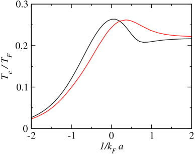
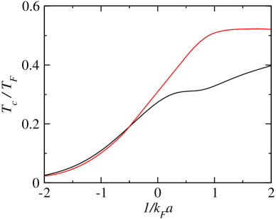
Figures 1 and 2 present comparisons of the superfluid transition temperatures in the two schemes for the homogeneous situation and in a trap. The black lines correspond to the BCS-Leggett scheme Chen et al. (2005a); Levin and Chen (2007) and the red lines are for the NSR approach as obtained in Reference Perali et al. (2004a). For the homogeneous case, it can be seen that there are only small quantitative differences, while in the trapped situation the BCS-Leggett scheme leads to considerable lower $T_{c}$ values slightly above unitarity. The root of the difference in the two calculational schemes lies physically in the fact that the BCS-Leggett scheme computes the transition temperature in the presence of a finite (pseudo)gap at $T_{c}$. In the NSR based scheme, these pair fluctuation effects do not appear as a pseudogap in the expression for $T_{c}$, but rather enter through corrections to the fermionic chemical potential $\mu^{*}$.

Section III.2 presented simple arguments which show that the ideal gas asymptote for $T_{c}$ is approached from below in the BCS-Leggett scheme, while it evidently is approached from above in the scheme of Nozieres and Schmitt-Rink. Both of these are mean field approaches and the behavior should not be compared with expectations Baym et al. (1999) based on a critical fluctuation description of true Bose systems which clearly include other physical mechanisms. Indeed, the fact that at $T_{c}$ there is a discontinuity in the NSR-based schemes suggests that this approach should be more suitable at $T\approx 0$, away from $T_{c}$.

Because of the different approaches to the ideal gas asymptote, in a trap one sees from Figure 2 that the differences between the two transition temperatures are more marked. The ideal gas asymptote is quickly reached in the NSR scheme very close to the point where $1/k_{F}a\approx 1$. In the BCS-Leggett scheme there is an extended regime at and on the BEC side of unitarity where $T_{c}$ is rather constant, and the asymptote is only reached for $1/k_{F}a$ considerably larger than its counterpart in the alternate school.

Figure 1: Comparison of $T_{c}/T_{F}$ as a function of inverse scattering length $1/k_{F}a$ in a homogeneous system within the BCS-Leggett scheme Chen et al. (2005a); Levin and Chen (2007) (black curve) and the Nozieres Schmitt-Rink Perali et al. (2004a) (red curve) scheme. The former has a maximum closer to unitarity and a dip close to the point where $\mu$ changes sign.

Figure 2: Comparison of $T_{c}/T_{F}$ in the trapped case for the two schools, using the local density approximation. As in the previous figure, the red curve is for the NSR scheme Perali et al. (2004a) and the black curve for the BCS-Leggett approach Chen et al. (2005a); Levin and Chen (2007).

V.3 Comparison Of Density Profiles

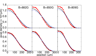
Figure 3 presents a plot from Ref. Perali et al. (2004b) of the axial density profiles in the BCS-Leggett ground state (dashed lines) as compared with the NSR-derived ground state (black lines) and the data points (shown in red) for ⁶Li. In axial profiles two of the three dimensions of the theoretical trap profiles were integrated out to obtain a one-dimensional representation of the density distribution along the transverse direction: $\bar{n}(x)\equiv\int dydz\,n(r)$. Three different values of the magnetic field near unitarity are shown, and the upper and lower panels correspond to slight changes in the number of atoms, $N$ which are assumed in the theoretical calculations. The figure shows that the agreement between theory and experiment is better for the smaller value of N. While the difference in the profiles associated with the two ground states is not particularly dramatic, it should be stressed that this difference is reflected in rather large changes in the coefficient $\beta$ discussed below. Overall the quantitative agreement between theory and experiment is seen to be better for the NSR-based ground state.

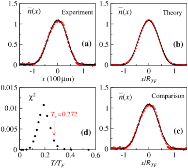
In Figure 4 are shown density profiles at finite temperatures for the BCS-Leggett case, from Reference Stajic et al. (2005b). The experimental data and theory correspond to roughly $T/T_{F}=0.19$. These profiles are estimated to be within the superfluid phase ($T_{c}\approx 0.3T_{F}$ at unitarity). This figure presents Thomas-Fermi fits Kinast et al. (2004b) to the experimental (4a) and theoretical (4b) profiles as well as their comparison (4c), for a chosen $R_{TF}=100\leavevmode\nobreak\ \mu m$, which makes it possible to overlay the experimental data (circles) and theoretical curve (line). Finally Fig. 4d indicates the relative $\chi^{2}$ or root-mean-square (rms) deviations for these TF fits to theory. This figure was made in collaboration with the authors of Ref. Kinast et al. (2004b). To probe the deviations from a TF functional form, in Fig. 4d, the (relative) rms deviation, or $\chi^{2}$, from the TF fits as a function of $T$ is plotted. $\chi^{2}$ increases rapidly below $T_{c}$ and reaches a maximum around $0.7T_{c}$. Quite good agreement between theory and experiment is observed here in the finite $T$ profiles.

Figure 3: Nozieres Schmitt-Rink based results for ground state profiles. Shown is a comparison between experimental and theoretical axial density profiles from Ref. Perali et al. (2004b). Experimental data from Ref. Bartenstein et al. (2004b) (dots) are shown for three different values of the magentic field B tuning. Theoretical results for NSR theory Perali et al. (2004b) at T=0 (solid lines) and for BCS-Leggett theory (dashed lines) are shown for the same corresponding parameters. The upper (lower) panels refer to the estimated number of atoms $N=4\times 10^{5}$ ($N=2.3\times 10^{5}$).

Figure 4: (color online) BCS-Leggett results for temperature dependent profiles of (a) experimental one-dimensional spatial profiles (circles) and TF fit (line) from Ref. Kinast et al. (2004b), (b) TF fits (line) to theory at $T\approx 0.7T_{c}\approx 0.19T_{F}$ (circles) and (c) overlay of experimental (circles) and theoretical (line) profiles, as well as (d) relative rms deviations ($\chi^{2}$) associated with these fits to theory at unitarity. The circles in (b) are shown as the line in (c). The profiles have been normalized so that $N=\int\bar{n}(x)dx=1$, and we set $R_{TF}=100\leavevmode\nobreak\ \mu$m in order to overlay the two curves. $\chi^{2}$ reaches a maximum around $T=0.19T_{F}$.

V.4 Addressing $\beta$ Effects

One of the most widely used milestones for assessing crossover theories is the numerical value obtained for the coefficient $\beta$. At unitarity the chemical potential must scale with the Fermi energy with a coefficient of proportionality

$$\mu=(1+\beta)E_{F}.$$ (93)

In the BCS-Leggett ground state $\beta\approx-0.41$. By contrast experimental data Bartenstein et al. (2004b) suggest an answer which is closer to Monte Carlo calculations Carlson et al. (2003) $\beta=-0.56$. Calculations Perali et al. (2004b) based on NSR-1 yield $\beta=-.545$, which is in quite good agreement with experiment. In the NSR-2 scheme (based on the thermodynamical potential with the non-variational contribution included), the same good agreement with experiment (and Monte Carlo) was presented Hu et al. (2006, 2007); Diener et al. (2008).

The BCS-Leggett- based scheme, as it has been implemented here, can be seen to ignore Hartree effects, just as is consistent with the ground state wavefunction. This is a shortcoming of the scheme and in the context of the formalism presented here, one can trace it to Eq. (34). This approximation, in effect, includes only pairing correlations in the self energy. Correlations that are not associated with pairing, such as Hartree effects have been omitted. With the full T-matrix formalism as outlined in Section III.1, it should be clear that this assumption can be avoided and is not fundamental to the physical picture presented here. However, dropping this simplification does lead to considerable numerical complexity. We note that the NSR-based theories both above and below $T_{c}$ include these non-pairing correlations in a fairly automatic way. In some limited contexts, they have also been included in the BCS-Leggett based theory Jankó et al. (1997); Maly et al. (1999a, b).

One can think of these omitted correlations as entering via Eq. (28) when the pair susceptibility is assumed Bruun and Baym (2004) to include only two bare Green’s functions. Most recently, it has been shown that these “$G_{0}G_{0}$” correlations are responsible for some important physical observations in the context of gases which are so strongly polarized that superfluidity is driven away Schunck et al. (2007). A bound state associated with the minority spins is found to occur Lobo et al. (2006); Combescot et al. (2007) in these highly imbalanced gases, which is responsible Punk and Zwerger (2007); Massignan et al. (2008) for anomalies in the RF spectra Schunck et al. (2007).

In summary, it is possible to estimate the size of these Hartree corrections, if one goes beyond Eq. (34) and includes the effects deriving from “$G_{0}G_{0}$” correlations, noted above. This will have to be done in future calculations for better quantitative comparisons of various properties, including $\beta$.

	NSR -1	NSR-2	BCS-Leggett	“Answer”
scatt. length ratio: $a_{B}/a$	2.0	$\approx$ 0.55	2.0	0.6 (exact calc.)
$\beta=\frac{\mu}{E_{F}}-1$	-0.545	-0.59	-0.41	-0.55, (from experiment)
$N_{c}$ at T=0, $1/k_{F}a=2$		0.84	0.99	0.96 (Monte Carlo)
$N_{c}$ at T=0, $1/k_{F}a=\infty$		0.48	0.69	0.58 (Monte Carlo)

Table 2: Quantitative Comparisons among the different schools. References for each number are listed in the first row from left to right: Ref. Pieri and Strinati (2005), Ref. Hu et al. (2007), Ref. Viverit et al. (2004), and Ref. Petrov et al. (2004). For the second row from left to right the references are: Ref. Perali et al. (2004b), Ref. Hu et al. (2007), Ref. Viverit et al. (2004) and Ref. Bartenstein et al. (2004b). For the third row from left to right the references are Ref. Fukushima et al. (2007), Ref. Astrakharchik et al. (2005) and Ref. Astrakharchik et al. (2005). Finally in the last row from left to right the references are Ref. Fukushima et al. (2007), Ref. Astrakharchik et al. (2005) and Ref. Astrakharchik et al. (2005).

V.5 Condensate Fraction and “Quantum Depletion”

It is interesting to contemplate the concept of “quantum depletion” in a fermionic system, particularly as one approaches the BEC. It is generally believed that the BCS-Leggett theory is to be distinguished from that based on NSR (which is closer to Bogoliubov theory) because of the neglect of quantum depletion. However, because of the presence of unpaired fermions, the condensate fraction will automatically show less than 100% condensation, except in the deepest BEC. Similarly, in the BCS regime this condensate fraction is vanishingly small. Establishing the degree to which “quantum depletion” is present in a Fermi gas is, thus, a subtle issue.

We begin with the BCS-Leggett ground state. Following earlier work Yang (1962), at $T=0$, the pair wavefunction is defined as $F_{\bf k}\equiv\langle N-2|c_{-{\bf k}\downarrow}c_{{\bf k}\uparrow}|N\rangle$, where $c_{{\bf k}\sigma}$ is the fermion annihilation operator for $\sigma=\uparrow,\downarrow$. It can be shown that in this ground state we have $F_{\bf k}=u_{\bf k}v_{\bf k}$, where the coefficients are $u^{2}_{\bf k},v^{2}_{\bf k}=[1\pm(\epsilon_{\mathbf{k}}-\mu)/E_{\bf k}]/2$ and $E_{\bf k}=\sqrt{(\epsilon_{\mathbf{k}}-\mu)^{2}+\Delta^{2}}$. The condensate fraction at $T=0$ is

$$N_{c}=\sum_{\bf k}|F_{\bf k}|^{2}=\int d{\bf r}|F({\bf r})|^{2}.$$ (94)

Here $F({\bf r})=\sum_{\bf k}F_{\bf k}\exp(i{\bf k}\cdot{\bf r})$. This pair density reflects off-diagonal-long-range-order. There have been a number of numerical calculations of this quantity over the entire BCS-BEC crossover Astrakharchik et al. (2005) and the agreement with direct Monte Carlo schemes Astrakharchik et al. (2005) is not unreasonable, as will be summarized below.

It is natural to try to extend this picture to finite temperature, taking the quantity $F_{\bf k}=T\sum_{\omega_{n}}F(i\omega_{n},{\bf k})=u_{\bf k}v_{\bf k}[1-2f(E_{\bf k})]$ as a measure of the pair density. We stress that this is not related to off-diagonal long range order, but rather contains the contributions from condensed and non-condensed pairs, through the decoupling of $\Delta^{2}$ into $\Delta_{sc}^{2}$ and $\Delta_{pg}^{2}$. One has, thus,

$$n_{pair}=\Delta^{2}[1-2f(E_{\bf k})]^{2}/4E_{\bf k}^{2},\leavevmode\nobreak\ \leavevmode\nobreak\ \leavevmode\nobreak\ T\neq 0.$$ (95)

To emphasize that there is no unique representation of the pair fraction away from the BEC limit, we note that Eq. (38) provides another natural decomposition We can rewrite this equation representing the total density of fermions $n$ in the form

$$n=2Z\Delta^{2}+2\sum_{\mathbf{k}}f(\epsilon_{\mathbf{k}}-\mu)$$ (96)

or equivalently

$$n=2Z\Delta_{sc}^{2}+2Z\Delta_{pg}^{2}+2\sum_{\mathbf{k}}f(\epsilon_{\mathbf{k}}-\mu),$$ (97)

from which

$$n_{pair}=2Z\Delta_{sc}^{2}+2Z\Delta_{pg}^{2},$$ (98)

can be obtained. There are three terms on the right hand side of Eq. (97). The second term corresponds to the density of fermions in the non-condensed pairs. The first term may be identified as $N_{c}=2Z\Delta_{sc}^{2}$, representing an alternative way of quantifying the density of fermions in the condensate, and the third term may be identified as the density of remaining (unpaired) fermions, $n_{f}=2\sum_{\mathbf{k}}f(\epsilon_{\mathbf{k}}-\mu)$. This decomposition is of interest, in part because it relates more directly to the decomposition of pairing contributions and free fermions introduced in the original NSR paper.

Recent calculations of $N_{c}$ Taylor et al. (2006); Fukushima et al. (2007) have also been presented using the NSR-2 approach, where the fraction is found to be somewhat smaller than in the BCS-Leggett state. Importantly, the difference between these two results for $N_{c}$ is viewed as a possible way to represent quantum depletion, which is naturally larger in NSR based theories as compared to the BCS-Leggett counterpart.

V.6 Effects of First Order Transitions

Essentially all NSR-based theories, as well as some which claim higher levels of consistency, report first order transitions fir . These effects presumably originate in the same way as their counterparts in true Bose systems treated at the Bogoliubov Shi and Griffin (1998) or Popov level. We outline the origin of these first order effects in Appendix C. They lead to derivative discontinuities in the density profiles at the condensate edge Giorgini et al. (1997a) and are thus, not as problematic in the case of a trapped gases as compared to a homogeneous system. This is particularly the case in the BEC where bimodality is present and one would expect signatures of the condensate edge.

Despite this theoretical framework, experiments show a behavior which is far from first order. One of the most striking features about the unitary gases is that there is so little indication of the phase transition and thus no evidence for first order behavior. This is seen by noting the historical difficulties encountered in establishing whether a particular experiment is performed in the superfluid or normal phase. In the absence of population imbalance, the unitary gas profiles are featureless Kinast et al. (2005) with no clear bi-modality or other indications of a condensate edge. Similarly, RF spectroscopic studies of the pairing gap show a smooth behavior Chin et al. (2004) from high $T$ to temperatures well below $T_{c}$. As a consequence, $T_{c}$ is difficult to identify, although important thermodynamical measurements, have indeed, indicated a phase transition Kinast et al. (2005).

These theoretically generated first order effects become even more difficult to reconcile with the fact that in BCS- BEC crossover, the pseudogap, which appears well above $T_{c}$ leads to an even smoother transition than in strict BCS theory (which also is of second order). Thus a first order transition in systems undergoing BCS-BEC crossover can be viewed as somewhat problematic, except, perhaps if attention is restricted to a narrow temperature range. This points to an advantage of the BCS-Leggett based approach where the density profiles are rather featureless and well fit to a Thomas Fermi form. A related advantage is that without first order transitions one can arrive at a theoretical basis Carr et al. (2004); Chen et al. (2005b) for adiabatic sweep thermometry. This is an experimental technique Chen et al. (2006); Zwierlein et al. (2004) which has been rather widely discussed. Using the theoretically determined entropy, it is possible to arrive at reasonable estimates of a final temperature, based on an experimentally known initial temperature connected by an adiabatic sweep.

V.7 Quantitative Comparisons

Quantitatively, the NSR-based approaches appear to have some advantage, although there are variations depending on how the number equation is implemented (either via NSR-1 or NSR-2). Table 2 summarizes specific key numbers which have been used to assess the different schools. Listed in the first row is the scattering length ratio associated with the inter-boson and inter-fermion interactions, while the second row compares the quantity $\beta$ defined in Eq. (93) which is associated with the unitary limit. Finally, the third and fourth rows address the value of the condensate fraction in the ground state in the near-BEC and very deep BEC. This is relevant to quantifying the degree of quantum depletion. We have previously addressed our concerns about NSR-2 which, through Eq. (88), builds on inconsistencies associated with the fact that the gap equation does not satisfy the variational condition. Rather we argue in favor of the approach we call NSR-1 which uses Eq. (67). While there seems to be considerable interest in the community in comparing numbers such as those shown in Table 2, because of just these concerns about more fundamental issues, we are of the opinion that it may be premature to give too much weight to the numerical comparisons shown in Table 2. Instead we attach greater importance to Table 1 for assessing a given theory and for indicating new directions for improvement.

VI Summary

One of the major goals of this review has been to clarify the genesis of a large number of contributions to the theoretical literature by associating them clearly with one or the other theoretical approaches to BCS-BEC crossover. We stress that these two theoretical schemes are different in the ground state and in their thermal properties. One should, thus, avoid the tendency to present results from the Leggett BCS ground state and simultaneously use the Nozieres Schmitt-Rink calculations for treating $T\neq 0$ aspects of BCS-BEC crossover.

It was also our goal to summarize the major strengths and weaknesses within these two schools. While it clearly includes bosonic degrees of freedom, there is a concern about the Leggett-BCS theory which concern derives from the fact that this approach does not yield a Bogoliubov-like or sound mode dispersion for the non-condensed pair excitations. Formally, this is a consequence of the associated T-matrix description of the $q\neq 0$ pairs, which drops higher order terms and which are needed to couple the condensate and pair excitations. Although it has not been seen as yet FOO , this sound-like excitation spectrum could show up in future experiments on unitary gases, particularly through power law dependences in thermodynamics. On the positive side, calculations in this BCS-Leggett phase are very tractable; one can readily handle inhomogeneities such as vortices (through the Bogoliubov deGennes approach); one can introduce trap effects, as well as population imbalance and address all temperatures $T$.

For the NSR based schemes a comparably major problem is that there is no satisfactory mean field theory for the weakly interacting Bose gas which works at all temperatures. The NSR based school is based on this Bose gas mean field starting point and this introduces unphysical first order transitions which, at least around $T_{c}$, will interrupt the smooth crossover from BCS to BEC and limit the applicability of theory to specified ranges of temperature. On the positive side, it is believed that this scheme, which works best at low temperatures, will produce the better ground state and allow more quantitative comparison with experiment at $T\approx 0$.

With these weaknesses identified, each of these schools has a large agenda in hand for future research. In the short term the BCS-Leggett scheme should be readily extended to include additional non-pairing contributions to the self energy (such as Hartree effects) which will make it more favorable for quantitative comparisons. Similarly, in the short term, the NSR-based approach should be extended to implement the inclusion of Popov like correlations, and thereby include corrections to the BCS gap equation (which treats the fermions as non-interacting). In the longer term one would hope that NSR scheme (which approaches the crossover from the BEC end and oversimplifies the fermionic dispersion) and the BCS-Leggett scheme (which approaches the crossover form the BCS end and oversimplifies the bosonic dispersion), will ultimately be unified. It is also to be expected that experiments will guide the way.

Appendix A Details of the T-matrix calculations

The T-matrix is $t_{pg}^{-1}(Q)=[U^{-1}+\chi(Q)]$. Near $T_{c}$ can it be expanded near $Q=0$ in the form

$$t_{pg}(\mathbf{q},\Omega)=\frac{1}{Z(\Omega-q^{2}/2M^{*})+\mu_{pair}+i\Gamma_{Q}}$$ (99)

after analytic continuation ($i\Omega_{l}\rightarrow\Omega+i0^{+}$). The pair chemical potential $\mu_{pair}$ vanishes below $T_{c}$. The relaxation term $i\Gamma_{Q}$ is neglected near $T_{c}$ in most applications. Firstly we calculate $Z$.

$$Z=\frac{\partial t_{pg}^{-1}}{\partial\Omega}\Big{|}_{\Omega=0,q=0}=\frac{1}{2\Delta^{2}}\left[n-2\sum_{\mathbf{k}}f(\epsilon_{\mathbf{k}}-\mu)\right].$$ (100)

The effective mass of pairs, $M^{*}$, is given by

$$\frac{1}{2M^{*}} = \frac{1}{6Z}\frac{\partial^{2}t^{-1}_{pg}(\mathbf{q},0)}{\partial\mathbf{q}^{2}}\Big{|}_{q=0}.$$ (101)

Here

$$\frac{\partial^{2}t^{-1}_{pg}(\mathbf{q},0)}{\partial\mathbf{q}^{2}}\Big{|}_{q=0} = -\frac{1}{2\Delta^{2}}\sum_{\mathbf{k}}\Bigg{\{}2f(\epsilon_{\mathbf{k}}-\mu)\Big{[}(\nabla_{\bf k}^{2}\epsilon_{\mathbf{k}})+4\Big{(}\frac{\epsilon_{\mathbf{k}}-\mu}{\Delta^{2}}\Big{)}(\nabla_{\bf k}\epsilon_{\mathbf{k}})^{2}\Big{]}-2f(E_{\bf k})\Big{[}\Big{(}\frac{\epsilon_{\mathbf{k}}-\mu}{E_{\bf k}}\Big{)}(\nabla_{\bf k}^{2}\epsilon_{\mathbf{k}})+$$ (102)

$$2\Big{\{}\frac{(E_{\bf k}^{2}+(\epsilon_{\mathbf{k}}-\mu)^{2})}{\Delta^{2}E_{\bf k}}\Big{\}}(\nabla_{\bf k}\epsilon_{\mathbf{k}})^{2}\Big{]}+4f^{\prime}(\epsilon_{\mathbf{k}}-\mu)(\nabla_{\bf k}\epsilon_{\mathbf{k}})^{2}-\Big{(}1-\frac{\epsilon_{\mathbf{k}}-\mu}{E_{\bf k}}\Big{)}(\nabla_{\bf k}^{2}\epsilon_{\mathbf{k}})+$$

$$\Big{(}\frac{2E_{\bf k}}{\Delta^{2}}\Big{)}\Big{(}1-\frac{\epsilon_{\mathbf{k}}-\mu}{E_{\bf k}}\Big{)}^{2}(\nabla_{\mathbf{\bf k}}\epsilon_{\mathbf{k}})^{2}\Bigg{\}}.$$

Appendix B Details on Eqs. (77) and (80)

We review how Eqs. (77) and (80) are derived following Pieri and Strinati (2005). The Dyson’s equation, Eq.(32) in Ref.Pieri and Strinati (2005), is

$$\hat{G}_{11}(K) = -\hat{G}_{22}(-K)=\hat{G}^{o}_{11}(K)+\hat{G}^{o}_{11}(K)[\Sigma_{11}(K)\hat{G}_{11}(K)+\Sigma_{12}(K)\hat{G}_{21}(K)],$$

$$\hat{G}_{12}(K) = \hat{G}_{12}(K)=\hat{G}^{o}_{11}(K)[\Sigma_{11}(K)\hat{G}_{12}(K)+\Sigma_{12}(K)\hat{G}_{22}(K)].$$ (103)

Following the approximation shown in Eq. (78), the self-energy becomes

$$\Sigma_{11}(K) \approx \frac{\bar{\Delta}_{pg}^{2}}{i\omega_{n}+\xi_{\bf k}},\mbox{ }\Sigma_{22}(K)\approx\frac{\bar{\Delta}_{pg}^{2}}{i\omega_{n}-\xi_{\bf k}}.$$ (104)

In the BEC limit, $\Delta_{sc}/|\mu^{*}|\ll 1$ and we assume this also holds for $\bar{\Delta}_{pg}/|\mu^{*}|$. Then $\hat{G}_{11}(K)$

$$= \frac{i\omega_{n}+\xi_{\bf k}-\frac{\bar{\Delta}_{pg}^{2}}{i\omega_{n}-\xi_{\bf k}}}{\left(i\omega_{n}-\xi_{\bf k}-\frac{\bar{\Delta}_{pg}^{2}}{i\omega_{n}+\xi_{\bf k}}\right)\left(i\omega_{n}+\xi_{\bf k}-\frac{\bar{\Delta}_{pg}^{2}}{i\omega_{n}-\xi_{\bf k}}\right)-\Delta_{sc}^{2}}$$ (105)

$$= -\frac{(i\omega_{n}+\xi_{\bf k})(\omega_{n}^{2}+\xi_{\bf k}^{2}+\bar{\Delta}_{pg}^{2})}{(\omega_{n}^{2}+\xi_{\bf k}^{2}+\bar{\Delta}_{pg}^{2})^{2}+\Delta_{sc}(\omega_{n}^{2}+\xi_{\bf k}^{2})}$$

$$= -\frac{i\omega_{n}+\xi_{\bf k}}{\omega_{n}^{2}+\xi_{\bf k}^{2}+\bar{\Delta}_{pg}^{2}+\Delta_{sc}^{2}\frac{\omega_{n}^{2}+\xi_{\bf k}^{2}}{\omega_{n}^{2}+\xi_{\bf k}^{2}+\bar{\Delta}_{pg}^{2}}}$$

$$\approx -\frac{i\omega_{n}+\xi_{\bf k}}{\omega_{n}^{2}+\xi_{\bf k}^{2}+\bar{\Delta}_{pg}^{2}+\Delta_{sc}^{2}}.$$

Here we made the approximation, which is valid in the BEC limit,

$$\frac{\omega_{n}^{2}+\xi_{\bf k}^{2}}{\omega_{n}^{2}+\xi_{\bf k}^{2}+\bar{\Delta}_{pg}^{2}}=1-\frac{\bar{\Delta}_{pg}^{2}}{\omega_{n}^{2}+\xi_{\bf k}^{2}+\bar{\Delta}_{pg}^{2}}\approx 1.$$ (106)

The off-diagonal fermion Green’s function $\hat{G}_{12}(K)$

$$= -\frac{\Delta_{sc}}{\left(i\omega_{n}-\xi_{\bf k}-\frac{\bar{\Delta}_{pg}^{2}}{i\omega_{n}+\xi_{\bf k}}\right)\left(i\omega_{n}+\xi_{\bf k}-\frac{\bar{\Delta}_{pg}^{2}}{i\omega_{n}-\xi_{\bf k}}\right)-\Delta_{sc}^{2}}$$ (107)

$$= \frac{\Delta_{sc}(\omega_{n}^{2}+\xi_{\bf k}^{2})}{(\omega_{n}^{2}+\xi_{\bf k}^{2}+\bar{\Delta}_{pg}^{2})^{2}+\Delta_{sc}^{2}(\omega_{n}^{2}+\xi_{\bf k}^{2})}$$

$$= \frac{\Delta_{sc}}{\omega_{n}^{2}+\xi_{\bf k}^{2}+2\bar{\Delta}_{pg}^{2}+\Delta_{sc}^{2}+\frac{\bar{\Delta}_{pg}^{4}}{(\omega_{n}^{2}+\xi_{\bf k}^{2})}}$$

$$\approx \frac{\Delta_{sc}}{\omega_{n}^{2}+\xi_{\bf k}^{2}+2\bar{\Delta}_{pg}^{2}+\Delta_{sc}^{2}}.$$

Note that the corresponding gap equation, Eq. (81), derived from this expression is different from the BCS gap equation when $E_{\bf k}$ is defined as $\sqrt{\xi_{\bf k}^{2}+\Delta_{sc}^{2}+\bar{\Delta}_{pg}^{2}}$.

Appendix C First order transitions in boson mean field theories

It is well known Giorgini et al. (1997b); Andersen (2004) that mean field theories of the weakly interacting Bose gas are associated with unphysical first order transitions. It is, thus, often argued that these theories should only be applied at temperatures much lower than $T_{c}$. Since the same issues arise with BCS-BEC crossover theories of the extended Nozieres Schmitt-Rink school (based on the Hartree-Fock-Bogoliubov or Popov approximations), it is useful to understand the physical origin of these first order effects.

We summarize here the central issues which lead to first order transitions:

1. The BEC transition temperature predicted by mean field theories is the same as the BEC temperature of an ideal Bose gas, $T^{0}_{BEC}$.

2. Below $T^{0}_{BEC}$, interaction effects are found to suppress thermal excitations. This suppression arises from interaction effects in the dispersion relation which lead to a systematic increase in the excitation energy, relative to the non-interacting gas. In addition there is a change in the phase space weighting factor. In combination, these two effects importantly yield a smaller fraction of non-condensed bosons (or a larger condensate fraction).

3. As a consequence, if one plots the condensate fraction obtained from generic mean field theory as a function of $T$, one sees that it tends towards $T^{0}_{BEC}$ by overshooting and then bending back towards $T^{0}_{BEC}$ at the highest temperatures below the transition. This double valued behavior is then associated with a first order transition.

Fig. 5 shows the condensate fraction (solid line) as a function of temperature as obtained from the Popov approximation. The bend-over which indicates a first order transition can be seen clearly. As a comparison, the condensate fraction of a non-interacting gas of bosons is also presented (dashed curve). Here one sees a smooth second order phase transition.

Figure 5: Condensate fraction $n_{0}/n$ as a function of dimensionless temperature $T/T^{0}_{BEC}$. Solid and dashed lines correspond to results obtained from the Popov approximation and the theory of non-interacting bosons, respectively.

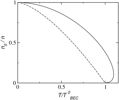
We can take these ideas over to the BCS-Leggett approach to BCS-BEC crossover (which is the only case where a first order transition is not seen). It is rather straightforward to see the analogies with the Bose gas through the gap equation: $\Delta^{2}=\Delta_{sc}^{2}+\Delta_{pg}^{2}$ in conjunction with Eq. (35) (and in some situations also with Eq. (37)). Here, too, following the interacting Bose gas logic we will also end up with an unphysical first order transition which means that the smooth crossover at finite $T$ is interrupted for some range of temperatures below and near $T_{c}$.

Appendix D Ward Identity Analysis of the number equation

The Ward identity is given by

$$Q\cdot\lambda(K,K_{+}) = G_{0}^{-1}(K)-G_{0}^{-1}(K_{+}),$$

$$Q\cdot\Lambda(K,K_{+}) = G^{-1}(K)-G^{-1}(K_{+}).$$ (108)

Here $G_{K}=[G_{0}^{-1}(K)-\Sigma(K)]^{-1}$ is the full fermion Green’s function. The full vertex is obtained by choosing a set of diagramms consistent with gauge invariance. These are shown in Fig. 6 and specified in the caption. Now we would like to show that this set of diagrams satisfy the Ward identity and does not contribute to the Meissner effect if the correct form of number equation is used.

Figure 6: The full vertex is approximated by these diagrams. The first one on the right hand side is the bare vertex, the second one is the “MT” diagram, and the last one is the “AL” diagram. Hollow and solid dots denote full and bare vertices. Solid lines and wavy lines correspond to propagator of non-interacting fermions and t-matrix, respectively.

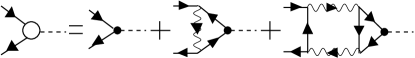
The expressions of those diagrams in Fig. 6 are

$$\lambda(K,K_{+}) = (2\mathbf{k}+\mathbf{q},1),$$ (109)

$$MT(K,K_{+}) = \sum_{P}t(P)G_{0}(P-K_{+})\times$$

$$\lambda(P-K_{+},P-K)G_{0}(P-K),$$

$$AL(K,K_{+}) = -2\sum_{L,P}t(P)t(P_{+})G_{0}(P-K)\times$$

$$G_{0}(P-L)G_{0}(L)\lambda(L,L_{+})G_{0}(L_{+}).$$

The factor $2$ in the AL diagram comes from the fact that the vertex can be inserted in one of the two particle propagators in the T-matrix. By taking inner produc with $Q$ they becomes

$$Q\cdot MT(K,K_{+}) = \sum_{P}t(P)G_{0}(P-K_{+})[G_{0}^{-1}(P-K_{+})-$$ (110)

$$G_{0}^{-1}(P-K)]G_{0}(P-K),$$

$$= -[\Sigma(K_{+})-\Sigma(K)].$$

$$Q\cdot AL(K,K_{+}) = -2\sum_{L,P}t(P)t(P_{+})G_{0}(P-K)G_{0}(P-L)G_{0}(L)[G_{0}^{-1}(L)-G_{0}^{-1}(L_{+})]G_{0}(L_{+}),$$ (111)

$$= -2\sum_{P}t(P)t(P_{+})G_{0}(P-K)[\chi(P_{+})-\chi(P)],$$

$$= 2[\Sigma(K_{+})-\Sigma(K)].$$

In deriving these results, Eqs.(109) and the identity $\chi(P_{+})-\chi(P)=t^{-1}(P_{+})-t^{-1}(P)$ are useful. Therefore $Q\cdot(MT+AL)=\Sigma(K_{+})-\Sigma(K)$. It is straighforward to show that the approximated vertex $\Lambda=\lambda+MT+AL$ satisfies the Ward identity. Since these diagrams are normal state diagrams, one can take the limit $Q\rightarrow 0$ and obtain

$$[MT(K,K)+AL(K,K)]_{\mu}=\frac{\partial\Sigma(K)}{\partial K_{\mu}}.$$ (112)

This is an important identity in the derivation of the absence of Meissner effect in the normal state.

The Meissner effect occurs if the static response kernel does not vanish, which is equivalent to the existence of a superfluid density. To show that the approximation for the full vertex does not contribute to the Meissner effect, it suffices to show that in the normal state

$$\left(\frac{n}{m}\right)_{xx}-P_{xx}(0)=0.$$ (113)

Here the density is calculated as ($\alpha,\beta=x,y,z$)

$$\left(\frac{n}{m}\right)_{\alpha\beta} = 2\sum_{K}\frac{\partial^{2}\xi_{k}}{\partial K_{\alpha}K_{\beta}}G(K)$$

$$= -2\sum_{K}\frac{\partial\xi_{k}}{\partial K_{\alpha}}\frac{\partial G(K)}{\partial K_{\beta}}$$

$$= -2\sum_{K}\frac{\partial\xi_{k}}{\partial K_{\alpha}}G^{2}(K)\left[\frac{\partial\xi_{k}}{\partial K_{\beta}}+\frac{\partial\Sigma(K)}{\partial K_{\beta}}\right].$$

We assume that surface terms can be neglected. The current-current correlation function at $Q=0$ is

$$P_{\alpha\beta}(0) = -2\sum_{K}G^{2}(K)[\lambda(K,K)+MT(K,K)+$$ (115)

$$AL(K,K)]_{\beta}\lambda(K,K)_{\alpha}$$

$$= -2\sum_{K}G^{2}(K)\frac{\partial\xi_{k}}{\partial K_{\alpha}}\left[\frac{\partial\xi_{k}}{\partial K_{\beta}}+\frac{\partial\Sigma(K)}{\partial K_{\beta}}\right],$$

where we used $\lambda(K,K)_{\alpha}=\frac{\partial\xi_{k}}{\partial K_{\alpha}}$.

Thus the two contributions cancel each other and there is no Meissner effect in the normal state.

This work is supported by NSF PHY-0555325 and NSF-MRSEC Grant No. DMR-0820054. We thank G.C. Strinati, A. Perali, P. Pieri, R.Hulet, and D. Wulin for helpful communications.

References

- Greiner et al. (2003) M. Greiner, C. A. Regal, and D. S. Jin, Nature 426, 537 (2003).
- Jochim et al. (2003) S. Jochim et al., Science 302, 2101 (2003).
- Regal et al. (2004) C. A. Regal, M. Greiner, and D. S. Jin, Phys. Rev. Lett. 92, 040403 (2004).
- Zwierlein et al. (2004) M. W. Zwierlein, C. A. Stan, C. H. Schunck, S. M. F. Raupach, A. J. Kerman, and W. Ketterle, Phys. Rev. Lett. 92, 120403 (2004).
- Zwierlein et al. (2005) M. W. Zwierlein, J. R. Abo-Shaeer, A. Schirotzek, and W. Ketterle, Nature 435, 170404 (2005).
- Kinast et al. (2004a) J. Kinast, S. L. Hemmer, M. E. Gehm, A. Turlapov, and J. E. Thomas, Phys. Rev. Lett. 92, 150402 (2004a).
- Bartenstein et al. (2004a) M. Bartenstein, A. Altmeyer, S. Riedl, S. Jochim, C. Chin, J. H. Denschlag, and R. Grimm, Phys. Rev. Lett. 92, 203201 (2004a).
- Kinast et al. (2005) J. Kinast, A. Turlapov, J. E. Thomas, Q. J. Chen, J. Stajic, and K. Levin, Science 307, 1296 (2005).
- Bourdel et al. (2004) T. Bourdel, L. Khaykovich, J. Cubizolles, J. Zhang, F. Chevy, M. Teichmann, L. Tarruell, S. J. Kokkelmans, and C. Salomon, Phys. Rev. Lett. 93, 050401 (2004).
- Partridge et al. (2005) G. B. Partridge, K. E. Strecker, R. I. Kamar, M. W. Jack, and R. G. Hulet, Phys. Rev. Lett. 95, 020404 (2005).
- Randeria (1995) M. Randeria, in Bose Einstein Condensation, edited by A. Griffin, D. Snoke, and S. Stringari (Cambridge Univ. Press, Cambridge, 1995), pp. 355–92.
- Chen et al. (2005a) Q. J. Chen, J. Stajic, S. N. Tan, and K. Levin, Phys. Rep. 412, 1 (2005a).
- Levin and Chen (2007) K. Levin and Q. Chen, in Ultra-cold Fermi Gases, edited by M. Inguscio, W. Ketterle, and C. Salomon (Italian physical society, 2007), p. 751.
- Leggett (2006) A. J. Leggett, Nature Physics 2, 134 (2006).
- Perali et al. (2002) A. Perali, P. Pieri, G. C. Strinati, and C. C, Phys. Rev. B 66, 024510 (2002).
- Eagles (1969) D. M. Eagles, Phys. Rev. 186, 456 (1969).
- Leggett (1980) A. J. Leggett, in Modern Trends in the Theory of Condensed Matter (Springer-Verlag, Berlin, 1980), pp. 13–27.
- Nozières and Schmitt-Rink (1985) P. Nozières and S. Schmitt-Rink, J. Low Temp. Phys. 59, 195 (1985).
- Friedberg and Lee (1989a) R. Friedberg and T. D. Lee, Phys. Lett. A 138, 423 (1989a).
- Friedberg and Lee (1989b) T. Friedberg and T. D. Lee, Phys. Rev. B 40, 6745 (1989b).
- Chen et al. (1998a) Q. J. Chen, I. Kosztin, B. Jankó, and K. Levin, Phys. Rev. Lett. 81, 4708 (1998a).
- Micnas and Robaszkiewicz (1998) R. Micnas and S. Robaszkiewicz, Cond. Matt. Phys. 1, 89 (1998).
- Ranninger and Robin (1996) J. Ranninger and J. M. Robin, Phys. Rev. B 53, R11961 (1996).
- Uemura (1997) Y. J. Uemura, Physica C 282-287, 194 (1997).
- Renner et al. (1998) C. Renner, B. Revaz, K. Kadowaki, I. Maggio-Aprile, and O. Fischer, Phys. Rev. Lett. 80, 3606 (1998).
- Deutscher (1999) G. Deutscher, Nature 397, 410 (1999).
- Junod et al. (1999) A. Junod, A. Erb, and C. Renner, Physica C 317-318, 333 (1999).
- Lee et al. (2006) P. A. Lee, N. Nagaosa, and X. G. Wen, Rev. Mod. Phys. 78, 17 (2006).
- Randeria (1998) M. Randeria, in Models and Phenomenology for Conventional and High-temperature Superconductivity, edited by G. Iadonisi, J. R. Schrieffer, and M. L. Chiafalo, Società Italiana di Fisica Bologna, Italy (IOS Press, 1998), vol. 136 of Proc. Int’l School of Physics ”Enrico Fermi” Courses, pp. 53–75.
- Jankó et al. (1997) B. Jankó, J. Maly, and K. Levin, Phys. Rev. B 56, R11407 (1997).
- Micnas et al. (1990) R. Micnas, J. Ranninger, and S. Robaszkiewicz, Rev. Mod. Phys. 62, 113 (1990).
- Trivedi and Randeria (1995) N. Trivedi and M. Randeria, Phys. Rev. Lett. 75, 312 (1995).
- Chen et al. (2001) Q. J. Chen, K. Levin, and I. Kosztin, Phys. Rev. B 63, 184519 (2001).
- Chen et al. (1998b) Q. J. Chen, I. Kosztin, B. Jankó, and K. Levin, Phys. Rev. Lett. 81, 4708 (1998b).
- Milstein et al. (2002) J. N. Milstein, S. J. J. M. F. Kokkelmans, and M. J. Holland, Phys. Rev. A 66, 043604 (2002).
- Ohashi and Griffin (2002) Y. Ohashi and A. Griffin, Phys. Rev. Lett. 89, 130402 (2002).
- Griffin and Ohashi (2003) A. Griffin and Y. Ohashi, Phys. Rev. A 67, 063612 (2003).
- Pieri et al. (2004a) P. Pieri, L. Pisani, and G. C. Strinati, Phys. Rev. Lett. 92, 110401 (2004a).
- Kosztin et al. (1998) I. Kosztin, Q. J. Chen, B. Jankó, and K. Levin, Phys. Rev. B 58, R5936 (1998).
- Chen et al. (1999) Q. J. Chen, I. Kosztin, B. Jankó, and K. Levin, Phys. Rev. B 59, 7083 (1999).
- Stajic et al. (2004) J. Stajic, J. N. Milstein, Q. J. Chen, M. L. Chiofalo, M. J. Holland, and K. Levin, Phys. Rev. A 69, 063610 (2004).
- Kinnunen et al. (2004) J. Kinnunen, M. Rodriguez, and P. Törmä, Science 305, 1131 (2004).
- Perali et al. (2003) A. Perali, P. Pieri, and G. C. Strinati, Phys. Rev. A 68, 031601R (2003).
- Pieri and Strinati (2000) P. Pieri and G. C. Strinati, Phys. Rev. B 61, 15370 (2000).
- Perali et al. (2004a) A. Perali, P. Pieri, L. Pisani, and G. C. Strinati, Phys. Rev. Lett. 92, 220404 (2004a).
- Perali et al. (2004b) A. Perali, P. Pieri, and G. C. Strinati, Phys. Rev. Lett. 93, 100404 (2004b).
- Diener et al. (2008) R. B. Diener, R. Sensarma, and M. Randeria, Phys. Rev. A 77, 023626 (2008).
- Andrenacci et al. (2003) N. Andrenacci, P. Pieri, and G. C. Strinati, Phys. Rev. B 68, 144507 (2003).
- Shi and Griffin (1998) H. Shi and A. Griffin, Phys. Rep. 304, 1 (1998).
- Andersen (2004) J. O. Andersen, Rev. Mod. Phys 76, 599 (2004).
- (51) P. Pieri, L. Pisani, and G. C. Strinati, Phys. Rev. B 70, 094508 (2004); R. Haussmann, W. Rantner, S. Cerrito, and W. Zwerger, Phys. Rev. A 75, 023610 (2007); N. Fukushima, Y. Ohashi, E. Taylor, and A. Griffin, ibid. 75, 033609 (2007); H. Hu, P. D. Drummond, and X. J. Liu, Nat. Phys. 3, 469 (2007).
- Kosztin et al. (2000) I. Kosztin, Q. J. Chen, Y.-J. Kao, and K. Levin, Phys. Rev. B 61, 11662 (2000).
- Machida and Koyama (2005) M. Machida and T. Koyama, Phys. Rev. Lett. 94, 140401 (2005).
- Chien et al. (2006a) C. C. Chien, Y. He, Q. J. Chen, and K. Levin, Phys. Rev. A 73, 041603 (2006a).
- Sensarma et al. (2006) R. Sensarma, M. Randeria, and T. L. Ho, Phys. Rev. Lett. 96, 090403 (2006).
- (56) J. Kinnunen, L. M. Jensen, and P. Törmä, Phys. Rev. Lett. 96, 110403 (2006); K. Machida, T. Mizushima, and M. Ichioka, ibid 97, 120407 (2006); T. Mizushima, M. Ichioka, and K. Machida, arXiv:0705.3361; R. Sensarma, W. Schneider, R. B. Diener, and M. Randeria, arXiv:0706.1741.
- Sheehy and Radzihovsky (2006) D. E. Sheehy and L. Radzihovsky, Phys. Rev. Lett. 96, 060401 (2006).
- De Silva and Mueller (2006) T. N. De Silva and E. J. Mueller, Phys. Rev. A 73, 051602(R) (2006).
- Chien et al. (2006b) C.-C. Chien, Q. J. Chen, Y. He, and K. Levin, Phys. Rev. Lett. 97, 090402 (2006b).
- (60) G. B. Partridge, W. Li, Y. A. Liao, R. G. Hulet, M. Haque, and H. T. C. Stoof, Phys. Rev. Lett. 97, 190407 (2006).
- Chien et al. (2007) C.-C. Chien, Q. J. Chen, Y. He, and K. Levin, Phys. Rev. Lett. 98, 110404 (2007).
- Deutscher (2008) G. Deutscher, New Superconductors: From Granular to High Tc (World Scientific, 2008).
- Tan and Levin (2006) S. N. Tan and K. Levin, Phys. Rev. A 74, 043606 (2006).
- Petrov et al. (2004) D. S. Petrov, C. Salomon, and G. V. Shlyapnikov, Phys. Rev. Lett. 93, 090404 (2004).
- Stajic et al. (2003) J. Stajic, A. Iyengar, Q. J. Chen, and K. Levin, Phys. Rev. B 68, 174517 (2003).
- Cote and Griffin (1993) R. Cote and A. Griffin, Phys. Rev. B 48, 10404 (1993).
- Belkhir and Randeria (1992) L. Belkhir and M. Randeria, Phys. Rev. B 45, 5087 (1992).
- Maly et al. (1999a) J. Maly, B. Jankó, and K. Levin, Physica C 321, 113 (1999a).
- He et al. (2007) Y. He, C.-C. Chien, Q. Chen, and K. Levin, Phys. Rev. B 76, 224516 (2007).
- Norman et al. (2007) M. R. Norman, A. Kanigel, M. Randeria, U. Chatterjee, and J. C. Campuzano, Phys. Rev. B 76, 174501 (2007).
- Chubukov et al. (2007) A. V. Chubukov, M. R. Norman, A. J. Millis, and E. Abrahams, Phys. Rev. B 76, 180501(R) (2007).
- Chen and Levin (2008) Q. Chen and K. Levin, Phys. Rev. B 78, 0200513(R) (2008).
- Stajic et al. (2005a) J. Stajic, Q. J. Chen, and K. Levin, Phys. Rev. A 71, 033601 (2005a).
- Viverit et al. (2004) L. Viverit, S. Giorgini, L. P. Pitaevskii, and S. Stringari, Phys. Rev. A 69, 013607 (2004).
- Haussmann (1993) R. Haussmann, Z. Phys. B 91, 291 (1993).
- Dalfovo et al. (1999) F. Dalfovo et al., Rev. Mod. Phys. 71, 463 (1999).
- Pieri and Strinati (2003) P. Pieri and G. C. Strinati, Phys. Rev. Lett. 91, 030401 (2003).
- Spuntarelli et al. (2007) A. Spuntarelli, P. Pieri, and G. C. Strinati, Phys. Rev. Lett. 99, 040401 (2007).
- Miller et al. (2007) D. E. Miller, J. K. Chin, C. A. Stan, Y. Liu, W. Setiawan, C. Sanner, and W. Ketterle, Phys. Rev. Lett. 99, 070402 (2007).
- Combescot et al. (2006) R. Combescot, M. Y. Kagan, and S. Stringari, Phys. Rev. A 74, 042717 (2006).
- Pieri et al. (2004b) P. Pieri, L. Pisani, and G. C. Strinati, Phys. Rev. B 70, 094508 (2004b).
- Fetter and Walecka (1971) A. L. Fetter and J. D. Walecka, Quantum Theory of Many-Particle Systems (McGraw-Hill, San Francisco, 1971).
- Pieri and Strinati (2005) P. Pieri and G. C. Strinati, Phys. Rev. B. 71, 094520 (2005).
- Serene (1989) J. W. Serene, Phys. Rev. B 40, 10873 (1989).
- Hu et al. (2006) H. Hu, X. J. Liu, and P. D. Drummond, Europhys. Lett. 74, 574 (2006).
- Hu et al. (2007) H. Hu, P. D. Drummond, and X. J. Liu, Nature Phys. 3, 469 (2007).
- Brodsky et al. (2006) I. V. Brodsky, M. Y. Kagan, A. V. Klaptsov, R. Combescot, and X. Leyronas, Phys. Rev. A 73, 032724 (2006).
- Taylor et al. (2006) E. Taylor, A. Griffin, N. Fukushima, and Y. Ohashi, Phys. Rev. A 74, 063626 (2006).
- Fukushima et al. (2007) N. Fukushima, Y. Ohashi, E. Taylor, and A. Griffin, Phys. Rev. A 75, 033609 (2007).
- Haussmann et al. (2007) R. Haussmann, W. Rantner, S. Cerrito, and W. Zwerger, Phys. Rev. A 75, 023610 (2007).
- Micnas et al. (1995) R. Micnas, M. H. Pedersen, S. Schafroth, T. Schneider, J. Rodriguez-Nunez, and H. Beck, Phys. Rev. B 52, 16223 (1995).
- Yanase et al. (2003) Y. Yanase, J. Takanobu, T. Nomura, H. Ikeda, T. Hotta, and K. Yamada, Phys. Rep. 387, 1 (2003).
- Tchernyshyov (1997) O. Tchernyshyov, Phys. Rev. B 56, 3372 (1997).
- Benard et al. (1993) P. Benard, L. Chen, and A. M. S. Tremblay, Phys. Rev. B 47, 15217 (1993).
- Stajic et al. (2005b) J. Stajic, Q. J. Chen, and K. Levin, Phys. Rev. Lett. 94, 060401 (2005b).
- Baym et al. (1999) G. Baym, J.-P. Blaizot, M. Holzmann, F. Laloe, and D. Vautherin, Phys. Rev. Lett. 83, 1703 (1999).
- Kinast et al. (2004b) J. Kinast, A. Turlapov, and J. E. Thomas (2004b), preprint cond-mat/0409283.
- Bartenstein et al. (2004b) M. Bartenstein, A. Altmeyer, S. Riedl, S. Jochim, C. Chin, J. H. Denschlag, and R. Grimm, Phys. Rev. Lett. 92, 120401 (2004b).
- Carlson et al. (2003) J. Carlson, S. Chang, V. Pandharipande, and K. Schmidt, Phys. Rev. Lett. 91, 050401 (2003).
- Maly et al. (1999b) J. Maly, B. Jankó, and K. Levin, Phys. Rev. B 59, 1354 (1999b).
- Bruun and Baym (2004) G. M. Bruun and G. Baym, Phys. Rev. Lett. 93, 150403 (2004).
- Schunck et al. (2007) C. H. Schunck, Y. Shin, A. Schirotzek, M. W. Zwierlein, and W. Ketterle, Science 316, 867 (2007).
- Lobo et al. (2006) C. Lobo, A. Recati, S. Giorgini, and S. Stringari, Phys. Rev. Lett. 97, 200403 (2006).
- Combescot et al. (2007) R. Combescot, A. Recati, C. Lobo, and F. Chevy, Phys. Rev. Lett. 98, 180402 (2007).
- Punk and Zwerger (2007) M. Punk and W. Zwerger, Phys. Rev. Lett. 99, 170404 (2007).
- Massignan et al. (2008) P. Massignan, G. M. Bruun, and H. T. C. Stoof, Phys. Rev. A 77, 031601(R) (2008).
- Astrakharchik et al. (2005) G. E. Astrakharchik, J. Boronat, J. Casulleras, and S. Giorgini, Phys. Rev. Lett. 95, 230405 (2005).
- Yang (1962) C. N. Yang, Rev. Mod. Phys. 34, 694 (1962).
- Giorgini et al. (1997a) S. Giorgini, L. P. Pitaevskii, and S. Stringari, J. Low Temp. Phys. 109, 309 (1997a).
- Chin et al. (2004) C. Chin, M. Bartenstein, A. Altmeyer, S. Riedl, S. Jochim, J. H. Denschlag, and R. Grimm, Science 305, 1128 (2004).
- Carr et al. (2004) L. D. Carr, G. V. Shlyapnikov, and Y. Castin, Phys. Rev. Lett. 92, 150404 (2004).
- Chen et al. (2005b) Q. J. Chen, J. Stajic, and K. Levin, Phys. Rev. Lett. 95, 260405 (2005b).
- Chen et al. (2006) Q. J. Chen, C. A. Regal, M. Greiner, D. S. Jin, and K. Levin, Phys. Rev. A 73, 041601 (2006).
- (114) Although we note that thermodynamic measurements in trapped gases have not been able to detect unambiguously the sound mode signatures in entropy since most of the weight comes from free fermions at the trap edge Kinast et al. (2005).
- Giorgini et al. (1997b) S. Giorgini, L. P. Pitaevskii, and S. Stringari, J. Low Temp. Phys. 109, 309 (1997b).