Effects of $\beta$-Decays of Excited-State Nuclei on the Astrophysical r-Process

Abstract

A rudimentary calculation is employed to evaluate the possible effects of $\beta$-decays of excited state nuclei on the astrophysical r-process. Single particle levels calculated with the FRDM are adapted to the calculation of $\beta$-decay rates of these excited state nuclei. Quantum numbers are determined based on proximity to Nilson model levels. The resulting rates are used in an r-process network calculation in which a supernova hot-bubble model is coupled to an extensive network calculation including all nuclei between the valley of stability and the neutron drip line and with masses 1$\leq$A$\leq$283. $\beta$-decay rates are included as functional forms of the environmental temperature. While the decay rate model used is simple and phenomenological, it is consistent across all 3700 nuclei involved in the r-process network calculation. This represents an approximate first estimate to gauge the possible effects of excited-state $\beta$-decays on r-process freezeout abundances.

1 Introduction

The r-process is responsible for the synthesis of roughly half of all nuclei heavier than A$\sim$70 and all of the actinides [1, 2]. The solar system r-process abundances act as the canonical constraint to r-process theories as well as the prime indicator of the success of r-process models. Several r-process sites have been proposed; the hot-bubble region of a type II supernova (SNII) has been modeled fairly successfully. The composition of the environment in which the r-process occurs might be expected to have a profound effect on the final abundance distribution. Observations indicate that the r-process site is primary [3] and further evidence may suggest that the r-process is also unique [4]; it may occur in a single site or event. The uniqueness of the r-process site, however, remains a subject of study [5].

Nuclear properties also constrain the r-process, and the purpose of this work is the examination of one particular characteristic - $\beta$-decay - as it relates to the r-process. The $\beta$-decay inputs, and other nuclear physics inputs, have been shown [6, 7] to have important effects on the success or failure of r-process models. This is somewhat unfortunate, as properties of only a few nuclei on the neutron closed shells closer to stability have been experimentally determined, while data for the rest are relegated to calculation [1]. Of paramount importance is the determination of nuclear masses and $\beta$-decay rates. Nuclear mass formulae based on the microscopic properties of nuclei are slowly replacing the empirical droplet models, and these can change resulting reaction rates by factors as large as 10⁸ [8]. As well, the r-process path is affected by the choice of mass formula, since the path roughly follows a line of constant S_n [1].

A successful r-process calculation must predict an abundance peak for nuclei in the A$\sim$195 region - a difficulty over much of the r-process parameter space. However, as discussed below, $\beta$-decays from excited state nuclei may help to mitigate this difficulty. They do so by allowing the r-process to proceed at a faster rate, thereby enhancing the abundances at higher masses.

For the purposes of this study, the most recent semi-gross theory of $\beta$-decay [9] has been adapted to neutron-rich nuclei relevant to the r-process. The ability of this model to determine decay properties of an extremely wide range of nuclei with reasonable accuracy and speed makes it ideal for this preliminary calculation. In particular, the semi-gross theory has good agreement for very neutron-rich nuclei [10, 11]. It has also been used to improve the accuracy of decay rates for astrophysical calculations by incorporating first-forbidden transition strengths [12]. In its original form, the gross theory of $\beta$-decay assumed that the energy states of a nucleus consist of a smoothed distribution with transition strengths that peak at or near the energy of the isobaric analog state [13, 14]. Subsequent evolutions of the gross theory incorporated strength functions allowing for transitions of higher forbiddenness [15], as well as improvements over the original theory to include odd-odd effects [16], sum rules [17], even-odd mass differences [18], and improvements on the strength functions [19].

While the precision of the Fermi gas model used is consistent with that of the gross theory itself, more accurate models might be used. Recently, shell effects in the parent nucleons have been taken into account by using an energy distribution for single-particle states [9, 20]; this is denoted as the “semi-gross theory.” In these models, the energy distribution of the daughter states is still assumed to be smooth. Thus, the transition strength functions depend on the quantum numbers only of the initial parent states and are independent of the energy of the parent state; transition types are based on a statistical weight for a particular parent state to make a particular type of transition. The advantage of using single-particle strength functions is that quantum numbers can be assigned to the states easily, lending a better notion of the actual strength of each type of transition involved.

Since decay rates of nearly all of the nuclei along the r-process path have yet to be studied in a laboratory, r-process calculations rely heavily on calculated decay rates. Further, the temperature of the r-process environment ( 10⁹K) necessitates accounting for nuclei in excited states, especially given the expected high level density of these far-from-stability nuclei. Some of the effects that might be expected if one considers excited state nuclei in r-process simulations include increased (n,$\gamma$) and ($\gamma$,n) rates, which might shift the r-process path, but would tend to counteract each other as the r-process is generally presumed to proceed at (n,$\gamma$)$\leftrightarrow$($\gamma$,n) equilibrium, increased neutrino spallation rates, tending to enhance smoothing in post-processing, and increased beta-decay rates. However, at signicant excitation, neutron separation energies are low enough that neutron emission may be a dominant decay mode. This is discussed briefly along with the discussion of excited-state decays in the network calculation.

Section 2 of this paper is an overview of $\beta$-decay calculations and average properties in calculating decay rates calculated using the more recent semi-gross theory. This includes a brief review of the semi-gross theory of $\beta$-decay and a description of the calculations of single-particle states and their relationship to $\beta$-decay in §2.1. Energy levels are calculated in §2.2 using the Finite Range Droplet Model (FRDM). Results of $\beta$-decay calculations of excitated state nuclei with the adapted FRDM are discussed in §2.3, along with their potential astrophysical importance. Application of these results to an r-process network calculation is made in §3 with results from a model with several environmental parameter sets described in §4. Future work and possibilities are discussed in §5, along with experimental possibilities.

2 Average Nuclear Properties in $\beta$-Decay

Average theories of $\beta$-decay, such as the gross theory and the more recent semi-gross theory, make them useful in estimating and adapting decay rates of several nuclei to large systems such as astrophysical network calculations. The major assumption in these theories is that nuclear level densities are high enough to make integration over states a fairly accurate approximation by replacing the matrix elements with transition probability distribution functions. For example, the decay rate for Fermi and GT transitions, as calculated in the gross theory by Takahashi and Yamada, is given by [14]:

$$\lambda=\frac{m^{5}_{e}c^{4}}{2\pi\hbar^{7}}\int_{-Q}^{0}\int_{\varepsilon_{0}(E)}^{\varepsilon_{1}}\sum_{\Omega}D_{\Omega}(E,\varepsilon)f_{\Omega}(-E)\frac{dN_{1}}{d\varepsilon}W(E,\varepsilon)\,d\varepsilon\,dE$$ (1)

which integrates over the product of the transition probability function $D_{\Omega}(E,{\varepsilon})$ between a parent nucleus state at energy $\varepsilon$ and a daughter state with a transition energy $E$, the density of states $dN_{1}/d\varepsilon$ of the decaying nuclei; the weighting function of the final state nucleus W(E,$\varepsilon$), which imposes the Pauli exclusion principle on the rate calculation; and the form factor f_Ω(-E), which is the product of the emitted electron wave functions and the Fermi function for a transition of type $\Omega$. Terms used in the equations of this paper are summarized in Tables 1 - 2.

The density of parent states $\frac{dN}{dE}$ supplies information on the nucleons available for decay, while the weighting function controls the availability of the daughter states to which the nucleons can decay. In the case of an even number of daughter nucleons, the available energy levels are filled up to a value $\varepsilon_{1}$-Q, and in the case of an odd number, there is a hole at the highest energy in the ground state. Therefore, the weighting function is given by [14]:

$$\begin{array}[]{l@{\quad}l}{W(E,\varepsilon)}_{even}=\left\{\begin{array}[]{l@{\qquad\qquad}l}1&\varepsilon+E\geq\varepsilon_{1}-Q\\ 0&\varepsilon+E<\varepsilon_{1}-Q\end{array}\right.&\\ {}&\\ {W(E,\varepsilon)}_{odd~{}}=\left\{\begin{array}[]{l@{\qquad\qquad}l}1&\varepsilon+E\geq\varepsilon_{1}-Q+2\Delta\\ \frac{1}{n_{3}}&\varepsilon+E=\varepsilon_{1}-Q\\ 0&\mbox{otherwise}\end{array}\right.\end{array}$$ (2)

The value of n₃, the number of daughter nucleons promoted to the highest energy due to the pairing forces, is:

$$n_{3}=\int_{\varepsilon_{1}-Q}^{\varepsilon_{1}-Q+\Delta}\left(\frac{dN_{2}}{d\varepsilon}\right)\,d\varepsilon$$ (3)

where dN₂/d$\varepsilon$ is the density of states of protons (neutrons) in $\beta^{-(+)}$ decay and $\Delta$ is the pairing gap.

The decay must be energetically possible, so the lowest possible energy that a decaying nucleon can have is $\varepsilon_{1}$-Q-E, recalling that E is the (negative) transition energy of the decaying nucleon. Thus, $\varepsilon_{0}$ in Equation 1 equals $\varepsilon_{1}$-Q-E, removing that variable from the equation.

2.1 Single-Particle States

Although a smooth model is adaptable to decays, particularly from the ground-state, excited states present the added difficulty of potentially altering the strength functions. For an accurate treatment, an estimate of the quantum numbers of these states is made. In the initial calculation, discrete energy levels are used. Thus, the density of states for neutrons (protons) in $\beta^{-(+)}$ becomes:

$$\left(\frac{dN}{d\varepsilon}\right)_{N/Z}=\sum_{i}n_{i}\delta(\varepsilon-\varepsilon_{i})$$ (4)

where the value of n_i corresponds to the number of nucleons in each state i. For discrete Fermi states, the levels are two-particle levels with n=zero, one, or two. The weighting function W(E,$\varepsilon$) in Equation 1 can also be adjusted for single particle daughter levels. In the original gross theory, the weighting function takes on values between zero and one and is typically zero or one except at a few special points. If energy levels are discrete, then the value of the weighting function for a two particle level is either zero, one, or 0.5 for a level that is already filled, empty, or half-filled (containing a single nucleon) respectively. In this formulation, the weighting function corresponding to the availability of the proton (neutron) level structure of the daughter nucleus, in $\beta^{-(+)}$ depends on the energies of both the daughter nucleon levels $\varepsilon_{k}$ and the parent nucleon levels $\varepsilon_{i}$, because their difference is necessary to determine if the decay is energetically possible:

$$W(\varepsilon_{i},\varepsilon_{k})=n_{k}\theta(\varepsilon_{i}-\varepsilon_{k}\pm\Delta_{NP}-m_{e})$$ (5)

where the $\pm$ is for $\beta^{\mp}$-decay, m_e is the electron mass, and $\Delta_{NP}$ is the neutron-proton mass difference.

Each composite state is treated as a mixture of quantum states that will depend on the model used. Therefore, the mixture in a level i is characterized by a sum of eigenstates weighted by the coefficient $\omega$(i;n,$l$,$j$) as a function of the quantum numbers of n, $l$, $j$. For this study, the quantum numbers are for eigenstates of a spherical shell model based on a Woods-Saxon potential. The coefficients for a level i are normalized to unity:

$$\sum_{n,l,j}\omega(i;n,l,j)=1$$ (6)

for each level i. The description and calculation of weights, as well as the determination of single-particle states, are further discussed in §2.2.

Transition strength functions are then adjusted to accomodate the single particle states in the daughter nucleus. Discrete functions are used to specify the most probable location and quantum numbers of an available state. Then, the transition strength for a specific level i can be written as a sum of the product of weights for the parent and daughter levels, since levels in the daughter nucleus are now assigned. The transition strength for favored decays now becomes:

$$D_{\Omega}(E,\varepsilon)=D_{\Omega}(\varepsilon_{f},\varepsilon_{i})=\sum_{\zeta,\xi}\omega(i,\zeta)\omega(f,\xi)\Lambda_{\Omega}(\zeta,\xi)$$ (7)

where the function $\Lambda$ is used to designate the selection rules (for the set of quantum numbers $\zeta$ and $\xi$ of the initial state i and final state f respectively) which satisfy the transition type $\Omega$:

$$\Lambda_{F} = \delta\left(j_{f},j_{i}\right)\delta\left(l_{f},l_{i}\right)\delta\left(T_{0,f},T_{0,i}\mp{1}\right)$$

$$\Lambda_{GT} = \delta\left(j_{f},j_{i}\right)\delta\left(l_{f},l_{i}\right)\delta\left(\tau_{0,f},\tau_{0,i}\mp{1}\right)$$

$$+\delta\left(j_{f},j_{i}\pm{1}\right)\delta\left(l_{f},l_{i}\right)\delta\left(\tau_{0,f},\tau_{0,i}\mp{1}\right)$$

$$\Lambda_{1,V} = \delta\left(j_{f},j_{i}\pm{1}\right)\delta\left(l_{f},l_{i}\pm{1}\right)\delta\left(\tau_{0,f},\tau_{0,i}\mp{1}\right)$$

$$\Lambda_{1,A} = \delta\left(j_{f},j_{i}\right)\delta\left(l_{f},l_{i}\pm{1}\right)\delta\left(\tau_{0,f},\tau_{0,i}\mp{1}\right)$$ (8)

$$+\delta\left(j_{f},j_{i}\pm{1}\right)\delta\left(l_{f},l_{i}\pm{1}\right)\delta\left(\tau_{0,f},\tau_{0,i}\mp{1}\right)$$

$$+\delta\left(j_{f},j_{i}\pm{2}\right)\delta\left(l_{f},l_{i}\pm{1}\right)\delta\left(\tau_{0,f},\tau_{0,i}\mp{1}\right)$$

The strength functions are also normalized to satisfy the necessary sum rules [21]. For a single energy level, the Fermi and GT strength functions are normalized to unity:

$$\int^{\infty}_{-\infty}D_{F,GT}(E,\varepsilon)dE\rightarrow\sum_{f}D_{F,GT}(\varepsilon_{f},\varepsilon_{i})=1$$ (9)

while the vector and axial first-forbidden functions are normalized as [21]:

$$\sum_{f}D_{V,A}(\varepsilon_{f},\varepsilon_{i})=\frac{R^{2}}{5}$$ (10)

where R is the nuclear radius. By substituting into Equation 1, the decay rate for $\beta^{\mp}$ decay is now:

$$\lambda = \frac{m_{e}^{5}c^{4}}{C2\pi^{3}\hbar^{7}}\left\{\sum_{i}\sum_{k}n_{i}n_{k}\theta(\varepsilon_{i}-\varepsilon_{k}\pm{\Delta}_{NP}-m_{e})\right.$$ (11)

$$\times\left.\sum_{\zeta}\sum_{\xi}\sum_{\Omega}\omega(i;\zeta)\omega(k;\xi)\Lambda_{\Omega}(\zeta,\xi)\left|G_{\Omega}\right|^{2}\left(2l_{\Omega}+1\right)f_{\Omega}(E)\right\}$$

The variables $\zeta$, $\xi$, and $\Lambda_{\Omega}(\zeta,\xi)$ represent the quantum numbers associated with the states comprising the parent and daughter states respectively and the factor to satisfy the necessary selection rules, as mentioned above. The decay order is given by $l$. The summation over $\Omega$ is simply the sum over all possible transition orders in the decay. G_Ω is the appropriate coupling constant (vector or axial-vector) for the transition. The value of C is equal to 1 for allowed transitions and ($\hbar$/m_ec)² for first forbidden transitions, the only possibilities considered in this paper. The value E is the transition energy, and is simply the difference in parent and daughter energy states plus (minus) the neutron-proton mass difference and the electron mass in $\beta^{-(+)}$ decay.

The transition matrix elements for a nucleus are then calculated as:

$$\begin{array}[]{l@{\quad}l}\left|M_{\Omega}(E)\right|^{2}&=\left|M_{\Omega}(\varepsilon_{i}-\varepsilon_{k})\right|^{2}\\ &=\sum_{i}\sum_{k}\sum_{\zeta}\sum_{\xi}n_{i}n_{k}\omega(i;\zeta)\omega(k;\xi)\Lambda_{\Omega}(\zeta,\xi)\\ \end{array}$$ (12)

The daughter level k is determined by the parent level i, the transition energy E, and the transition order $\Omega$. The sum over quantum states $\zeta$ in the i^th parent level as well as the sum over states $\xi$ in the j^th daughter level are both necessary. Though the daughter state is constrained by the transition selection rules for a transition $\Omega$, there may be several quantum states so allowed, so the sum over states $\xi$ is necessary. As an example, the discrete transition strength matrix elements for ¹³²Sn are shown in Figures 1 - 3. One should note the characteristic broad peak corresponding to the GT matrix element (as compared to the Fermi matrix element, which has no viable transition strengths relevant for $\beta^{-}$ decay), as well as the double peak characteristic of the first-order transition elements.

It can be seen from Equation 11 that excited states are completely accounted for in the values n_i and n_k. This makes the utility of the equation obvious. As well, nuclear excitations can take the form of proton or neutron single-particle excitations without regard to the type of decay. The inclusion of selection rules is accomplished through a specification of quantum numbers of individual states. Furthermore, if all of the possible energy states above the Fermi surface are specified, the population of these states are assumed to be in thermodynamic equilibrium, and the partition function is then determined. Therefore, at temperatures peculiar to the r-process environment (or any environment), the values n_i and n_k can be substituted with the probability functions for a statistical ensemble in thermodynamic equilibrium.

2.1.1 Form Factors

Besides the calculation of single particle energies, the only remaining term in the rate equation is the f-function which, based on the order $\Delta{l}$, rank $\Delta{j}$, and vector nature of the transition (axial vector or vector) for $\beta^{\mp}$-decay is:

$$f_{l,j,A/V}(E)=\int_{1}^{W_{0}}F_{l,A/V}S_{l,j,A/V}^{\mp}pWq^{2}dW$$ (13)

where F_l,A/V is the Fermi function, which is taken to be the same in all cases; F_l,A/V=F₀, independent of $\Delta{l}$. The quantity S_l,j,A/V is the factor for the Coulomb interaction between the outgoing electron wave function and the nucleon wave functions. W is defined as the electron kinetic energy E_e/(m_ec²)$\pm$1 for $\beta^{\mp}$-decay, and W₀ corresponds to the maximum possible electron energy E for a transition. Also, the terms p and q are given by p=(W²-1)^1/2 and q=W₀-W. The forms of the wave function factors used are those of reference [15].

2.2 Calculation of Single-Particle States

2.2.1 Energy Levels of the Single-Particle States

The finite range droplet model (FRDM) with the Lipkin-Nogami (LN) pairing force is used to calculate single-particle levels for the various nuclei. The formula is referred to as a microscopic-macroscopic - or “mic-mac” model. The macroscopic part is a smooth function of proton number Z and neutron number N based on a finite range liquid drop model. The microcopic part is used to calculate individual shell energies and is based on a folded-Yukawa single-particle potential. The macroscopic part is described if reference [22]. It is based on the overall charge, mass, and the nuclear shape. The parametrized macroscopic part, as described in the reference is:

$$\begin{array}[]{l@{\quad}l}E_{mac}(Z,N,shape)=\\ +\Delta{M}_{H}Z+\Delta{M}_{n}N&\mbox{mass excess of hydrogen and neutron}\\ +\left({-a_{1}+J\bar{\delta}^{2}-\frac{1}{2}K\bar{\epsilon}^{2}}\right)A&\mbox{volume energy}\\ +\left({a_{2}+\frac{9}{4}\frac{J^{2}}{Q}\bar{\delta}^{2}\frac{B_{s}^{2}}{B_{1}}}\right)A^{2/3}&\mbox{surface energy}\\ +a_{3}A^{1/3}B_{k}&\mbox{curvature energy}\\ +a_{0}A^{0}&\mbox{A${}^{0}$ energy}\\ +c_{1}\frac{Z^{2}}{A^{1/3}}B_{3}&\mbox{Coulomb energy}\\ -c_{2}Z^{2}A^{1/3}B_{r}&\mbox{volume redistribution energy}\\ -c_{4}\frac{Z^{4/3}}{A^{1/3}}&\mbox{Coulomb exchange correction}\\ -c_{5}Z^{2}\frac{B_{w}B_{s}}{B_{1}}&\mbox{surface redistribution energy}\\ +f_{0}\frac{Z^{2}}{A}&\mbox{proton form factor correction}\\ {}&\mbox{to Coulomb energy}\\ -c_{a}\left({N-Z}\right)&\mbox{charge asymmetry term}\\ +W\left({\left|I\right|+\left\{\begin{array}[]{l@{\quad}l}1/A&\mbox{Z=N=odd}\\ 0&\mbox{otherwise}\end{array}\right.}\right)&\mbox{Wigner energy}\\ +\left\{\begin{array}[]{l@{\quad}l}\bar{\Delta}_{p}+\bar{\Delta}n-\delta_{np}&\mbox{Z and N odd}\\ \bar{\Delta}_{p}&\mbox{Z odd, N even}\\ \bar{\Delta}_{n}&\mbox{Z even, N odd}\\ 0&\mbox{Z and N even}\end{array}\right.&\mbox{average pairing energy}\\ -a_{el}Z^{2.39}&\mbox{energy of bound electrons}\end{array}$$ (14)

The parameters for this expression, as well as their derivations, are described extensively in [22], and will be described briefly here. Many of the constants used in this relationship are described in Table 3. Other derived quantities are given in the table, as well. The standard droplet model defines the shape-dependent quantities [23] as the surface energy $B_{s}$, the surface redistribution energy $B_{w}$, the curvature energy $B_{k}$, and the volume redistribution energy $B_{r}$. These are solved analytically by integrating the appropriate quantities over the surface of the nuclear volume:

$$\begin{array}[]{l@{\quad}l@{\quad}l}B_{s}&=&\frac{1}{4{\pi}r_{0}^{2}A^{2/3}}\int_{S}{dS}\\ B_{w}&=&\frac{225}{64{\pi}^{3}r_{0}^{6}A^{2}}\int_{S}{\left[\tilde{W}\left(\vec{r}\right)\right]^{2}dS}\\ B_{k}&=&\frac{1}{8{\pi}r_{0}A^{1/3}}\int_{S}{\left({\frac{1}{R_{1}}-\frac{1}{R_{2}}}\right)dS}\\ B_{r}&=&\frac{1575}{64{\pi}^{3}r_{0}^{7}A^{7/3}}\int_{V}{\left[\tilde{W}\left(\vec{r}\right)\right]d^{3}r}\\ \end{array}$$ (15)

where $R_{1}$ and $R_{2}$ are principal radii of curvature (two principal radii assume deformations having no higher than quadrupole terms in the macroscopic model). The volume term is specified as $\tilde{W}\left(\vec{r}\right)=W(r)-\tilde{W}$ and:

$$\begin{array}[]{l@{\quad}l@{\quad}l}W\left(\vec{r}\right)&=&\int_{V}{\frac{1}{\left|{\vec{r}-\vec{r}\prime}\right|}d^{3}r^{\prime}}\\ \tilde{W}&=&\frac{3}{4{\pi}r_{0}^{3}A}\int_{V}{W\left({\vec{r}}\right)d^{3}r}\end{array}$$ (16)

The quantities $B_{1}$ and $B_{3}$ are the relative generalized surface and Coulomb energies respectively for a deformed shape of volume $V=\frac{4\pi}{3}\left({r_{0}A}\right)^{3}$. These quantities are developed to treat nuclei under finite compressibility and diffuseness $a_{den}$. The generalized forms of these quantities are:

$$\begin{array}[]{l@{\quad}l}B_{1}&=\frac{1}{8\pi^{2}r_{0}^{2}a^{4}}\int\int_{V}{\left({2-\frac{\left|\vec{r}-\vec{r}^{\prime}\right|}{a}}\right)\frac{e^{\left|\vec{r}-\vec{r}^{\prime}\right|}/a}{\left|\vec{r}-\vec{r}^{\prime}\right|/a}d^{3}rd^{3}r^{\prime}}\\ B_{3}&=\frac{15}{32\pi^{2}r_{0}^{5}A^{5/3}}\int\int_{V}\frac{d^{3}rd^{3}r^{\prime}}{\left|\vec{r}-\vec{r}^{\prime}\right|}\left[{1-\left(1+\frac{1}{2}\frac{\left|\vec{r}-\vec{r}^{\prime}\right|}{a_{den}}\right)e^{\left|\vec{r}-\vec{r}^{\prime}\right|/a_{den}}}\right]\end{array}$$ (17)

These shape factors, along with their derivatives with respect to the radius are solved numerically in the FRDM, and the balance between the Coulomb energy, compressibility, and the surface tensions are found based on shape parameters taken from the deformation parameters in a folded Yukawa potential. For a spherical geometry, $B_{1}$ and $B_{3}$ are equal to 1 with the ranges $a$ and $a_{den}$ are equal to 0 - a sharp surface. The macroscopic constants in the FRDM have been determined based on a non-linear least squares fit requiring about 1000 iterations of the process of choosing parameters, recalculating potential surfaces, finding the fit, and re-adjusting parameters.

The microscopic portion of the model involves the individual shell terms plus the effective interaction pairing gaps for protons and neutrons[24, 25]:

$$\begin{array}[]{l@{\quad}l}\Delta_{G_{n}}&=\frac{r_{mic}B_{s}}{N^{1/3}}\\ \Delta_{G_{p}}&=\frac{r_{mic}B_{s}}{Z^{1/3}}\\ \end{array}$$ (18)

in which a constant level density is assumined in the vicinity of the Fermi energy level. The value of $r_{mic}$ is determined by a least-squares fit.

Finally, microscopic corrections to the FRDM are carried out by decoupling the shell and pairing potentials as well as the proton and neutron potentials. The single-particle potential is then the sum of the central potential $V_{1}$, which - as stated - is the folded Yukawa potential, the spin-obit potential $V_{s.o.}$, and the Coulomb central potential for protons $V_{C}$. Two-particle levels as a function of nucleon number are compared to those determined by the Nilson model (with no deformation) for the ¹³²Sn nucleus in Figure 4 showing a reasonable agreement between the two.

For a more complete description of the LN pairing interaction and microscopic interaction, the reader is referred to references [22] and to [25] and references therein.

In the present calculation, single particle levels are determined for both the parent and daughter nucleons. That is, transitions between specific levels are calculated for a nucleus with j parent nucleons and k daughter nucleons to a nucleus with j-1 parent nucleons and k+1 daughter nucleons. Thus, corrections to any shell and pairing energies are intrinsically accounted for.

2.2.2 Quantum Numbers of Single Particle States

A knowledge of the quantum numbers of each level enables one to calculate the order of a particular $\beta$ transition. However, as stated previously, a Fermi Gas model level at a specific energy may correspond to several shell model levels in the present formulation, so it may turn out to be a mixture of single-particle shell model eigenstates. The basis of states is assumed to be those of a spherical shell model with a Woods-Saxon potential [26]. The weight for each set of quantum numbers in a level is determined by the proximity of a level’s energy to that of a basis state. The overlap of the eigenfunctions at a shell level determines the strength of their presence in the level (Figure 5). The method of Nakata et al. is used to determine not only the quantum numbers of parent nucleons, but also those of daughter nucleons [9]. Triangular distribution functions centered on the energy of the states are defined:

$$H_{n,l,j}(\varepsilon)=\left\{\begin{array}[]{l@{\qquad\qquad}l}\frac{N_{n,l,j}}{q(A)}\left[1-\frac{|\varepsilon-\varepsilon_{n,l,j}|}{q(A)}\right]&-q(A)<\varepsilon-\varepsilon_{n,l,j}<q(A)\\ {}\\ 0&\mbox{otherwise}\end{array}\right.$$ (19)

where $\varepsilon_{n,l,j}$ is the energy of the eigenstate corresponding to the usual quantum numbers. The function is already normalized to N_n,l,j, which is equal to the degeneracy of a level, 2j+1. The width q(A) of the basis function of the $i^{th}$ level in a nucleus with $\mu$ levels is given by:

$$q(A)=6\frac{d_{i}}{d_{\mu}}$$ (20)

where d_i is the standard level spacing:

$$d_{i}\equiv\frac{2}{3\left({2i-2}\right)}\varepsilon_{i}^{0}$$ (21)

where $\varepsilon_{i}^{0}$ is the energy of the Fermi surface of the $i^{th}$ level. Since the values of $\varepsilon$ are allowed to vary smoothly, and scale smoothly with level, Fermi gas levels are appropriate to effect this scaling.

The total sum of the functions in Equation 19 is also defined:

$$G\left(\varepsilon\right)=\sum_{n,l,j}H_{n,l,j}(\varepsilon)$$ (22)

And G($\varepsilon$) is automatically normalized to the total number of nucleons. To find the coefficient $\omega$(i;n,l,J) in Equation 6 for the i^th single-particle level, it is necessary to normalize the function G($\varepsilon$) such that the overlap in the the region of the level is equal to two - the number of nucleons per level:

$$N_{i}\int_{\varepsilon^{-}}^{\varepsilon^{+}}G(\varepsilon)\,d{\varepsilon}=2$$ (23)

where the integration limits are the midpoints between the i^th level and adjacent levels:

$$\varepsilon^{\pm}=\frac{\varepsilon_{i}+\varepsilon_{i\pm 1}}{2}$$ (24)

For i=1 $\varepsilon^{-}$=0. The coefficient for a particular configuration of quantum numbers in the i^th level is then:

$$\omega(i;n,l,j)=\frac{1}{2N_{i}}\int_{\varepsilon^{-}}^{\varepsilon^{+}}H_{n,l,j}(\varepsilon)\,d\varepsilon$$ (25)

This method is diagrammed in Figure 5 [9]. The degeneracy of the spherical shell model level $\varepsilon_{n,l,j}$ is already accounted for in Equation 19 with the factor N_n,l,j. The selection rules in Equation 11 are then given by the function $\Lambda_{\Omega}(\zeta;\xi)$ and can now be easily determined, where $\Omega$ is the order and rank of the transition ($\Delta{l}$,$\Delta$j); $\zeta$ and $\xi$ represent the quantum numbers of the initial and final nucleon states respectively, (n_i,$l_{i}$,j_i;n_f,$l_{f}$,j_f). Thus, the selection rules can be simply stated as:

$$\Lambda(n_{i},l_{i},j_{i};n_{f},l_{f},j_{f})=\delta\left({l_{f},l_{i}{\pm}\Delta{l}}\right)\delta\left({j_{f},j_{i}\pm\Delta{j}}\right)$$ (26)

where the values of $\Delta{l}$ and $\Delta{J}$ depend on the initial and final state quantum numbers.

Because each state’s wave function is a sum of shell-model eigenstates, the smearing of single-state quantum numbers over several single-particle states is possible. The net result is still an average calculation of $\beta$-decay rates, but now individual particle and particle-hole excitations can be simulated by promoting an arbitrary nucleon to any available level. Further, the selection rules are now easily calculated using the method of the previous section.

2.2.3 Corrections in Pairing Energy Due to Decay

If the highest-level paired neutron decays, the other neutron in that level gains an amount of energy roughly equal to the pairing energy of that level. As well, paired neutrons in the next lowest level are then expected to reconfigure by both losing an amount of energy equal to the pairing energy of that level. Thus, the endpoint energy (taken to be positive in this respect) is changed by an amount equal to 2b_μ-1-b_μ just from the changes in the parent nucleus. (It is not necessary to include the energy of the decaying neutron since this is accounted for in the quantity $\varepsilon_{i}-\varepsilon_{f}$.)

Similarly, in the daughter nucleus, if the highest proton level (in $\beta^{-}$-decay) is unpaired, and a neutron decays to that level, then the highest original paired level loses its pairing energy for the two protons, while the level to which the neutron decays becomes the highest paired level, increasing the total endpoint energy by an amount b_μ, and the total energy available to the ejected electron changes by b_μ-2b_μ-1. (Again, the pairing energy of the decaying particle is not included for the same reasons mentioned above.)

2.3 Results of $\beta$-Decay Rate Calculations

Decay rates and Q-Values have been calculated with the FRDM in previous works [27]. The level of accuracy of these calculations is shown in Figures 6 and 7 for about 200 sample neutron-rich nuclei unstable against $\beta^{-}$decay for which the decay rates and Q-values are experimentally known. In Figure 6, the value of S is defined as:

$$S{\equiv}\log{\left(\frac{\lambda_{\mbox{calc}}}{\lambda_{\mbox{exp}}}\right)}$$ (27)

In each figure, most calculated rates fall within an order of magnitude of the true rate.

2.3.1 Excited State Decays

A next logical step is to calculate decay rates for nuclei in excited states. The present formulation gives no preferential treatment to nucleons in single-particle excited states. One simply needs to know the values of the excited levels and the vacant levels for Equations 4 and 5. The levels are already calculated from §2.2. Levels can be calculated beyond the maximum filled level in the ground state, although the simplicity of the model can render these values slightly different from their experimental counterparts.

In stellar environments, the probability of finding a nucleus in an excited state at a given temperature can be obtained from the partition function by knowing the spin and energy of the excited state. Since each particle level holds only two nucleons, the degeneracy of each level is two, and the quantum numbers are given by the level’s proximity to those of the spherical shell model (as described in §§2.2.2). The difference in energy:

$${\Delta}E={\sum_{i_{N,Z}=1}^{m}n_{n,i}^{*}\varepsilon_{i}^{*}-\sum_{i_{N,Z}=1}^{\mu}n_{n,i}^{0}\varepsilon_{i}^{0}}$$ (28)

where values with an ^∗ are those for an excited-state nucleus, while those with a ⁰ are those corresponding to a ground-state nucleus. The summation is taken over neutron and proton levels. The value m is the highest bound state level. The first term represents the total energy of the excited nucleus, and the second term is the total energy of the ground-state nucleus. The average decay rate of an isotope in a stellar environment is then the weighted sum over energy states [28]:

$$\lambda=\sum_{{\Delta}E}P({\Delta}E)\lambda({\Delta}E)$$ (29)

where P($\Delta$E) is calculated using the partition function.

Excited states and their decay rates have been calculated for several nuclei. A sample of the decay rates as a function of these states are shown for four nuclei in Figure 8. This figure shows the dependence of decay rates on excitation for an even-even nucleus (¹⁵⁰Ba), an odd-N nucleus (¹⁴⁹Ba), an odd-Z nucleus (¹⁴⁷Cs), and an odd-odd nucleus (¹⁵⁰La). One first notes the multiplicity of levels resulting from the splitting of states with spins higher than 1/2, a direct result of using levels with a degeneracy of two.

One also notes the apparent clustering of decay rates into bands. In the case of ¹⁵⁰Ba, one notes three major bands at $\frac{\lambda}{\lambda_{0}}\approx$0.75, 1, and 2 where $\lambda_{0}$ is the ground-state decay rate. This is due to the fact that single-particle levels are dominated by specific shell-model eigenstates in certain regions, as expected. In the case of ¹⁵⁰Ba, the first several single-particle neutron excitations above the ground-state contain large admixtures of the $i_{13/2}$ state, while those near the ground-state Fermi surface are predominantly in the $h_{9/2}$ state. In the case of transitions in this region, the decay order of the particle-hole configurations goes from GT to first-forbidden, thus reducing the decay rate. Single-particle excitations in certain energy regions are expected to have similar decay strengths. The band at $\frac{\lambda}{\lambda_{0}}\approx$2 is due to proton $\bar{\pi}g_{9/2}\pi{g}_{7/2}$ particle-hole configurations which do not change the transition order, but change the decay Q-value by opening up a hole at lower energies. The band at $\lambda/\lambda_{0}\approx$1 corresponds to $\bar{\nu}i_{13/2}\nu{i}_{11/2}$ configurations. Since this has very little impact on the highest-energy GT (or first-forbidden) transitions (to the $\pi{g}_{7/2}$ or $\pi{g}_{9/2}$ state), the overall transition rate is changed very little. It is expected that higher excitations will result in other band structures. However, since astrophysically interesting temperatures are below 1 MeV, the contribution to average decay rates from states much above this is small, so only lower excitations were studied.

Similarly, the band structures in the other nuclei shown can be explained in a similar manner. The band structures of other nuclei vary based on their individual structures. For example, ${}^{150}La$ has a band at $\frac{\lambda}{\lambda_{0}}<1$, but no band at $\frac{\lambda}{\lambda_{0}}>1$ (for the energies of interest). This nucleus has a higher deformation than ¹⁵⁰Ba, as well as an unpaired neutron and an unpaired proton. The lowest excitation energies are accomplished via neutron $\bar{\nu}h_{9/2}\nu{i}_{13/2}$ particle-hole configurations, but single-proton excitations are due primarily to the unpaired proton, which has little bearing on the available hole, but does account slightly for the vertical band structure in the figure; the rate increases with the transition energy for a single type of transition.

Of course, excitations can change the strength functions, as the order of a particular transition can be altered. In the case of ¹⁵⁰Ba, the GT strength function is shown for the ground state, a transition to the region dominated by the $\bar{\pi}g_{9/2}\pi{g}_{7/2}$ state, and an excited state dominated by the $\bar{\nu}h_{9/2}\nu{i}_{13/2}$ state in Figure 9. As expected, the neutron excitation lowers the overall GT transition strength, particularly at the highest transition energies, where the transition rate is highest. Conversely, the proton excitation increases the overall rate slightly at the lowest energies, while also increasing the Q-value. It should be noted in this case that, although the rate is doubled and the GT strength function for the proton excitation looks very similar to that of the ground-state, the average lifetime is still relatively low ($\sim$300ms), and the result is a small absolute increase in lifetime (to about 315ms). Overall, there are similar small changes in the first-forbidden strength functions, shown in Figure 10.

Given these figures, one cannot definitively state that excited-state nuclei decay at a higher rate than ground-state nuclei, as the transition order shift becomes important. The average decay rates of the nuclei in Figure 8 are plotted as a function of temperature in Figure 11, calculated using Equation 29. The decay rate of ¹³²Sn as a function of temperature is also plotted. While each nucleus behaves differently, it seems clear that the doubly-magic ¹³²Sn does exhibit a sharp increase in decay rate with temperature at higher temperature, most likely due to the fact that ¹³²Sn has closed proton and neutron shells. All single-particle excitations in ¹³²Sn are quite high in energy and open transitions that were previously Pauli-blocked. The transition strength functions for the first calculated excited state of ¹³²Sn are shown along with the ground-state functions in Figures 1-3 indicating greatly increased GT strengths even at high transition energy.

Finally, the effect of temperature on $\beta$-decay rates is evaluated as a function of the neutron-richness of the nucleus in Figure 13. In this figure, relative decay rates are plotted as a function of temperature for various Z on the same isobar A=162. For this isobaric chain, there may be a slight dependence on the stability of the nucleus. While more study is warranted, this may be of interest in suggesting that GT transitions of the highest level neutrons in the very neutron-rich nuclei along the r-process path are most likely not Pauli blocked, as they might be for the nuclei closer to stability. In this case, single-proton excitations will occupy states that a neutron would otherwise decay to. Nuclei closer to stability, on the other hand, have truncated GT strength functions. Thus, proton or neutron excitations are more likely to open transitions that were originally Pauli-blocked.

3 Effects of Excited-State Decays on the r-Process

Relative changes in decay rates along the r-process path are shown in Figure 12 for the line of constant neutron separation energy $S_{n}\approx 2.5$ MeV for three different temperatures. The effect is to increase slightly the relative ratios of the ground-state rates at lower mass. However, this effect is only slight ($<$10%) in temperature regimes relevant to the r-process. A network calculation is necessary to evaluate fully the magnitude of the effect on the r-process. The increase in the ¹³²Sn rate may be enough to make a significant difference in the final abundances, but this is not clear yet.

3.1 The Explosion Model

The r-process environment used in the present study is constructed in the semi-analytic model of the nutrino-driven winds of reference [31]. The mass flow out of the supernova hot-bubble region is treated as a spherically symmetric, steady flow around a neutron star of mass M and radius R in the Schwarzchild geometry, which is described [30] by the following sets of equations:

$$\dot{M} = 4\pi{r^{2}}\rho{u}$$

$$u\frac{du}{dr} = \frac{1}{\rho_{T}+P}\frac{dP}{dr}\left(1+u^{2}-\frac{2M}{r}\right)-\frac{M}{r^{2}}$$

$$\dot{q} = u\left(\frac{d\varepsilon}{dr}-\frac{P}{\rho_{b}}\frac{d\rho_{b}}{dr}\right)$$ (30)

where $\dot{M}$ is the mass outflow rate, $\rho_{b}$ is the baryon density, $\varepsilon$ is the specific internal energy, $u$ is the radial component of the four-velocity, and $\dot{q}$ is the net heating rate; $\dot{q}$ is positive just above the surface of the neutron star, decreasing roughly exponentially with radius. The total energy density $\rho_{T}$ is related to the baryon density by $\rho_{T}=\rho_{b}\left({1+\varepsilon}\right)$. In the above equations, the constants $\hbar$, $c$, $k_{B}$, and $G$ are equal to unity. In a stationary rest frame, the radial velocity of the expanding bubble is the product of the Lorentz factor and the radial component of the four-velocity:

$$v_{r}=u\left(1+u^{2}-\frac{2M}{r}\right)^{-\frac{1}{2}}$$ (31)

The net heating rate is determined by the sum of neutrino heating and cooling from the following reactions and their inverses:

$$\nu_{e}+n \leftrightarrow e^{-}+p$$

$$\bar{\nu}_{e}+p \leftrightarrow e^{+}+n$$

$$\nu_{i}+e^{-} \leftrightarrow \nu_{i}+e^{-}$$

$$\nu_{i}+e^{+} \leftrightarrow \nu_{i}+e^{+}$$

$$\bar{\nu}_{i}+e^{-} \leftrightarrow \bar{\nu}_{i}+e^{-}$$

$$\bar{\nu}_{i}+e^{+} \leftrightarrow \bar{\nu}_{i}+e^{+}$$

$$\nu_{i}+\bar{\nu}_{i} \leftrightarrow e^{-}+e^{+}$$ (32)

where the index $i$ corresponds to each neutrino flavor. The Newtonian forms of these heating and cooling rates are described in detail in references [6] and [29]. Since the mass flow is influenced by the properties of the proto-neutron star, the heating rate is strongly dependent on the neutrino luminosities and energies. Transformation of the solid angle from the reference frame of the neutron star to the r-process site leads to the correct form of the heating rate in the Schwarzchild geometry [31]. In this calculation, the neutrino luminosity $L_{\nu_{i}}$ is assumed to be the same for all neutrino flavors and the RMS energies are used; the energies for $\varepsilon_{\nu_{e}}$, $\varepsilon_{\bar{\nu}_{e}}$, $\varepsilon_{\nu_{\mu,\tau}}$, and $\varepsilon_{\bar{\nu}_{\mu,\tau}}$ are 12, 22, 34, and 34 MeV respectively.

Equations 3.1 are supplemented with the equations of state in the high-temperature limit taken from Qian and Woosley (1996):

$$P = \frac{11\pi^{2}}{180}T^{4}+\frac{\rho_{b}}{m_{N}}T$$

$$\varepsilon = \frac{11\pi^{2}}{60}T^{4}+\frac{3}{2}\frac{T}{m_{N}}$$ (33)

where $m_{N}$ is the nucleon rest mass.

Using Equations 3.1 and 3.1, the evolution of the hot bubble is followed. The adjustable parameters for solving the equations are $M$, $R$, and $\dot{M}$. The neutrino luminosity is taken to be 5 - 7$\times$10⁵¹erg s^-1. The equations are solved implicitly and the result is the velocity and thermodynamic quantities as a function of r (and hence, t). Any trajectory (velocity, temperature, and density as a function of radius) can be specified with the parameter set, and the entropy and dynamic timescale - parameters important to the r-process - are direct results of the evolution of the r-process environment. In this particular calculation, the approximation of a steady flow is used [31], which allows an analysis of the rarified region about the supernova core without requiring a tremendous amount of computational power.

For this model, a typical outer boundary temperature of T=0.1 MeV behind the shock at r$\approx$10,000 km, consistent with the theoretical result of the benchmark hydrodynamic simulations of the delayed-explosion of Type II supernovae [6] is used. Subsequent extended studies of the neutrino- driven wind [32, 33] have used the outer boundary condition that the mass ejection rate $\dot{M}$ (Equation 3.1) is taken to be 99% of its critical value (that is, the value for which wind velocity is supersonic). We therefore adopt the same outer boundary condition as that of ref. [32] with the core radius held constant at 10 km in the present calculations is used. The only two remaining hydrodynamical parameters are the core mass and the neutrino luminosity. From this, the dynamic timescale $\tau_{dyn}$, temperature, and density at any radius can be determined. From the temperature and density, the entropy is determined.

The nuclear reaction network used in this calculation [34, 35] is coupled to the output of the aforementioned hydrodynamic code. As shown in Figure 14, the network consists of about 3700 nuclei with Z$\leq$93 and includes all nuclei between the most proton-rich stable nuclei and the neutron drip line [34]. Possible reactions in this network are (n,$\gamma$), (p,$\gamma$), ($\alpha$,$\gamma$), (p,n), ($\alpha$,p), ($\alpha$,n), $\beta$-decay, $\beta$-delayed neutron emission, electon capture, and neutrino neutral- and charged-current interactions and their inverses [34]. These reactions are summarized in Figure 15. The effects of excited-state nuclei are included via the scaling of decay rates, as discussed below. Nucleosynthesis calculations begin at T₉=9, a sufficiently high temperature that a state of nuclear statistical equilibrium (NSE) exists, defined by the balance of strong and electromagnetic interactions. At this temperature matter is mostly in the form of free nucleons. The initial electron fraction Y_e is a parameter of the reaction network.

In order to maintain the consistency in the mass formula, the same formula used to calculate shell energies for $\beta$-decay rate calculations (i.e., the single-particle formula of TUYY [36])was used to calculate neutron separation energies, $\alpha$-particle separation energies, $\beta$-delayed neutron emission probabilities and ground-state $\beta$-decay rates for the nuclei shown in Figure 14. $\beta$-decay rates as a function of temperature were determined for nuclei with neutron separation energies less than about 2.75 MeV. (It is not very useful to calculate decay rates as a function of temperature for nuclei with $S_{n}>$2.75 MeV because, the r-process path does not pass through these nuclei until well after freezeout.) Of course, the neutron separation energies and capture rates are also affected by nuclear single-particle excitations. This becomes important especially along the r-process path where neutron separation energies are low. One may expect an increase in both the neutron emission rate as well as the capture rate for excited-state nuclei though capture and photoemission are in equilibrium in the classical r-process. However, single-neutron excitations cannot go above the neutron separation energy. For this reason, single-neutron excitations are kept realistically low (though multiple-particle excitations may be higher). Indeed, even at r-process temperatures, one does not expect a significant population of states above the neutron separation energy.

While the network calculation proceeds to Z=100, the mass formula used in this work has shell energies up to N=157. Therefore, neutron-rich nuclei with N$>$157 cannot be quantified, which effectively limits proton number Z to about 93. However, this is well past the A=195 peak in the r-process abundance distribution, and the effects of not including excited state rates for these very heavy nuclei have little effect on the abundances of the lighter nuclei. Also, it was found that the abundances of fissile nuclei along the path are very low at freezeout, so that the inclusion of fission cycling was ignored in this r-process model.

3.2 Excited State $\beta$-Decays in the Reaction Network

The inclusion of excited state $\beta$-decays into the reaction network can be computationally simple. Functional forms of decay rates with temperature were used. This allows a fairly accurate evaluation of the calculated rates of individual nuclei for temperatures between 0 and 6 billion K, while still maintaining the speed of the network calculation. Sixteen regions of the isotopic chart were found for which decay rates of nuclei in these regions have similar dependences on temperature. These regions are shown in Table Effects of $\beta$-Decays of Excited-State Nuclei on the Astrophysical r-Process. Nuclei represented in these figures have neutron separation energies S_n ranging between 0 and about 2.75 MeV. This sort of parametrization allows for a very reasonable first approximation of the change in decay rates over a large region of the isotopic chart.

The dependence on temperature for the above mentioned regions can be conveyed with a set of parameters fit to the formula:

$$\frac{\lambda}{\lambda_{0}}=E\left({FT_{9}+G}\right)\left[{A-\frac{B}{\exp{\left({C\left({T_{9}-D}\right)}\right)}+1}}\right]+{\alpha}\exp{\left({\beta{T_{9}}+\gamma{T_{9}^{2}}}\right)}$$ (34)

where $\lambda$ is the $\beta$-decay rate at temperature T₉ (defined to be the temperature in 10⁹ Kelvin), and the ground-state decay rate is $\lambda_{0}$.

The ratio in Equation 34 must be unity at T₉=0, so several of the parameters are dependent:

$$G = \frac{1}{E}$$

$$B = \left({A-1}\right)\left({\exp{\left({-CD}\right)}+1}\right)$$ (35)

so the parameter set is reduced to eight in number. Further, in using Equation 34 to fit the dependences of rates to temperature, two terms were necessary in the temperature region of interest. In actuality, only one of the two terms is present at a time. So if $E$ is non-zero, then $\alpha$ is zero and vice-versa. Also, $\alpha$ is limited to one of two values - 0 or 1 - leaving seven free parameters. The parameters for each of the regions mentioned above, along with the nuclei included in each region, are given in Table Effects of $\beta$-Decays of Excited-State Nuclei on the Astrophysical r-Process.

Two of the parameters in Table Effects of $\beta$-Decays of Excited-State Nuclei on the Astrophysical r-Process are functions of the nuclear proton number Z. These are the values of A for region 8 and the value of $\gamma$ for region 7a, listed in the table as $\tilde{A}(Z)$ and $\tilde{\gamma}(Z)$ respectively. This is a convenient way of representing these parameters over a very large isotopic region, as the functional form of the temperature dependence of decay rate changes slowly with Z. These parameters are given by:

$$\tilde{A}(Z) = 100.31-1.38Z$$

$$\tilde{\gamma}(Z) = 0.185-0.003Z$$ (36)

No odd-even effects are observed because Equation 34 is a ratio of rates, so any local odd-even effects would be minimized in the division. Variations in the parameters as a function of mass seem to be explainable in terms of local shell effects.

3.2.1 Uncertainty Associated With the Use of the Spherical Shell Model

It is worth mentioning the use and applicability of the spherical shell model in this formulation. One should not only consider effects on decay rates, but on the overall r-process. While it is difficult to compare to a more elaborate model in this work without utilizing such a model, a qualitative assesment is discussed here. Two things which are not necessarily mutually exclusive must be considered. The first is the accuracy of the decay rates used. The second is the applicability of the spherical shell model to the nuclei studied. In particular, one can estimate effects on individual transitions when one considers a Nilsson shell model with deformation. For this reason, nuclei which are presumed undeformed are compared to those which are considered to lie in regions of deformity in the isotopic chart (i.e., between closed shells) are discussed.

In estimating the accuracy of the calculated decay rates, one considers uncertainties in calculations for ground-state nuclei; the uncertainty in the decay rates may be estimated using Figure 6. The rms error in S (Equation 27) for all nuclei studied in this work with known $\beta^{-}$ decay rates has been calculated. The rms value S_rms=$\langle$S${}^{2}\rangle^{\frac{1}{2}}$ has for all nuclei, even-even nuclei, odd-N nuclei, odd-Z nuclei, and odd-odd nuclei to be 0.767, 0.569, 0.805, 0.745, and 0.872 respectively for the ground state nuclei, indicating reasonable agreement as shown in Figure 6 for at least the nuclei with known decay rates including those in regions of presumed deformity. The accuracy improves with rate as the presumed level density increases. For nuclei with $\lambda>$0.1 s^-1 the value of S_rms is 0.579 and decreases further to 0.467 for nuclei with $\lambda>$ 1 s^-1, indicating the improvement in the accuracy of this formulation for the r-process, in which the decay rates are larger. The agreement is also equally good for the few known neutron-rich isomers, though some caution is warranted here as the number of known isomeric states is small. As many of the nuclei studied were extremely neutron rich, the uncertainty in calculations is expected to be reasonable for those nuclei along the r-process path. In fact, the uncertainty is expected to decrease with single-particle level density. While reasonable, these errors may likely be reduced with a more realistic model.

In the case of non-deformed nuclei, the spherical shell model is believed to be a reasonable estimate of the decay rates. This is extremely important in the case of the r-process as the waiting points are localized about areas of lowest deformation; most of the r-process abundance is confined to these regions of the isotopic chart. Large uncertainties in the decay rates through the waiting points can result in drastic changes in the final distribution. For example, consider the A$\sim$130 abundance peak. If the decays rates of the r-process nuclei associated with this peak were much higher, then an increased flow through this peak would result, resulting in a much lower abundance of nuclei in this peak and a very large enhancement of the rare earth nuclei (130$<$A$<$190).

On the other hand, the portion of the r-process path thought to be responsible for the production of the rare-earth elements passes through a region of the isotopic chart associated with possibly large deformations. The overall effects on the final r-process abundance distribution due to changes in the decay rates of these nuclei is expected to be small as their contribution to the total abundance is small. In the case of these possibly deformed nuclei, single-particle levels in the Nilsson model may shift by as much as 0.5 MeV from those of the spherical shell model in cases of extreme deformation. However, single-particle levels are shifted in both the positive direction and the negative direction for protons and neutrons. Qualitatively, the net effect is to break degeneracies in closed shells while “spreading out” high localized single-particle level densities associated with closed shells.

Consider, for example, Figures 9 and 10 which show the calculated GT and first-forbidden strength functions for the ¹⁵⁰Ba nucleus for various excitations. If a more realistic structure model was used, the net result would be a spreading of the widths of the peaks of these functions as both the daughter and parent states would undergo shifts in both the positive and negative energies. While some of the strength function would shift to higher transition energies (more negative energies on the figure) resulting in contributions to higher decay rates, some would also shift to positive energies resulting in contributions to lower decay rates (and possibly - though unlikely - to states that cannot decay). By shifting the transition energy by an extreme amount of 0.5 MeV for a GT transition in Equation 11, it is estimated that the transition rates may change by as much as a factor of two. However, it must be carefully noted that this is for a shift of the entire GT transition strength in one direction for an extreme amount for only the most deformed nuclei. Thus, this factor is an upper limit for very deformed nuclei, and likely the error due to using a more accurate model is found using the rms values in S as discussed above. Certainly future work may concentrate on more realistic model calculations, though it will be seen from the next section that this may not be necessary as the results of the r-process calculations are more heavily dependent on uncertainties in the hydrodynamic conditions.

4 Results of the Network Calculation

The results from several hydrodynamic parameter sets, as well as electron fraction parameter values $Y_{e}$, were examined. These parameter sets are shown in Table 5. For each parameter set, the core mass in solar masses, core radius, neutrino luminosity, initial electron fraction, and whether or not $\beta$-delayed neutron emission is included are listed. Using these parameters and the calculations of reference [31] the dynamic timescale and the entropy in the expansion are constrained. Though still in agreement with current predictions, the dynamic timescales in these calculations are shorter than average. However, the entropy is lower, and no artificial increase in the entropy (as is often assumed) was required [6].

Each simulation is run until several seconds beyond freezeout. While this time is sufficient to gauge the gross features of the r-process abundance distribution, a longer simulation may have resulted in more post-processing, allowing for smoother abundance distributions. Figure 16 shows that model A underproduces the A$\sim$195 peak by a large amount. This is due primarily to the fact that the lower entropy in model A results in a very low neutron-to-seed ratio. Models B and C were chosen as intermediate points in the entropy-timescale phase space. Both produce a more acceptable r-process abundance distribution, although the A$\sim$195 peak is still underproduced. For comparison, the solar r-process abundance distribution is displayed in the figure. One notes some residual even-odd effects in the calculated distribution as the effects of smoothing may not be complete, though the gross features of the distribution are noted.

Results from models B and C are displayed in Figure 17 for both the hot (i.e., including excited-state decays, solid line) and cold (i.e., not including excited state decays, dashed line) models. The A$\sim$195 peak is most profoundly affected, along with the nuclei just below this mass region. From the relationship between the decay rates and temperature (Equation 34 and Table Effects of $\beta$-Decays of Excited-State Nuclei on the Astrophysical r-Process), it can be seen that decay rates of the nuclei in the region just below the A$\sim$195 peak (and - to a lesser extent - the region just below the A$\sim$130 peak) are quite sensitive to changes in temperature even at low temperatures. This is expected due to the high level densities of these nuclei (lying just below the N=126 and N=82 closed shells), as discussed in §2. Shell quenching has not been included in this calculation, though the effect is noted, and no conclusions can be drawn from this study to evaluate the effects of quenced closed shells far from stability. Other rates, however, are not as sensitive to temperature changes at low temperatures and, as the r-process progresses, these rates would drop to their ground-state values before those of the nuclei in the regions below the abundance peaks. The decay rates of nuclei in this region would increase relative to those of nuclei in other regions of the path, selectively depleting the abundances of nuclei in this region. This effect is displayed in Figure 12, in which nuclei in these two regions have large changes in decay rate as T₉ increases a small amount.

The lowering of the electron fraction in models F and G is a physically acceptable assumption given that the electron neutrinos and anti-neutrinos captured on nucleons before the beginning of the $\alpha$-process can alter the neutron excess $\eta$ via neutrino interactions on the free nucleons in NSE. In a steady-state, the electron fraction is [37]:

$$Y_{e}\approx\left({1+\frac{\langle{E_{\bar{\nu}_{e}}}\rangle}{\langle{E_{{\nu}_{e}}}\rangle}}\right)^{-1}$$ (37)

Given the neutrino energies assumed in the nucleosynthesis code, then a value as low as $Y_{e}$=0.35 may not be unexpected, though higher values have also been used.

The abundance distribution results of models F and G are shown in Figure 18. The A$\sim$195 peaks are more pronounced - closer to acceptable values - in both cases as compared to models B and C. Even more, abundances of nuclei with heavier masses are also increased, more closely matching the solar system abundance distribution in this region. As in previous models, the effect of excited state $\beta$-decays is still quite evident in both models, especially for the heavy nuclei with A$>$195. The ratios of peak abundances for these models are shown in Table 6. Both models have peak abundance ratios close to that of the solar system. Also, in both models, the A$\sim$195 peak is shifted closer in position to the solar system abundance peak. The slight decrease in Y_e, while still maintaining physically realistic values, combined with the use of excited-state $\beta$-decays, produces an r-process calculation with results that match the solar system distribution, with the exception of nuclei in the A$\sim$180 region, which seem to exhibit a deficiency in abundance.

Figures 17 and 18 suggest that the inclusion of excited-state $\beta$-decays results in a net shift of abundance from the region of nuclei just below the A$\sim$195 abundance peak into this abundance peak. Certainly, one notes that the more rapid decay rates in the region just below the abundance peaks results in a faster progression of the r-process through these nuclei. However, one should also note that the integrated abundances for nuclei with 180$<$A$<$200 is higher in the hot model by than in the cold model by 29%, indicating that overall abundance is increased in both the abundance peak and the region below this peak. This suggests that the increase in abundance in the A$\sim$195 abundance peak is only partially due to an increase in the decay rates of the nuclei associated with the region just below this peak. One must note that the overall abundance in the 180$<$A$<$200 region increases due to a flow of abundance into this region from the lower masses. This increased abundance can come from minute changes in abundance in the A$\sim$130 peak and from the mass region just below this peak. In the semi-log representation of Figures 17 and 18, it is seen that even small fractional changes in the abundance of the A$\sim$130 peak - with nearly an order of magnitude more abundance than the A$\sim$195 peak - can result in sizable changes in the 180$<$A$<$200 mass region. A similar comparison can be made between the abundance region just below the A$\sim$130 peak and the A$\sim$195 peak.

This brings up an interesting point regarding the net effect of rate increases with temperature in the r-process. Not surprisingly, figure 12 shows that decay rates for the closed-shell nuclei are only affected at high temperatures (corresponding to early stages in the r-process). Very early in the r-process, flow through the A$\sim$130 mass region increases relative to the remaining nulcei along the r-process path, populating the rare earth region. However, as temperature drops before freezeout, the relative flow through this mass region decreases, and the relative flow through the rare earth region is still higher, populating nuclei in the A$\sim$195 mass region. As the A$\sim$195 mass region is not populated until later (and cooler) in the r-process, the effects of excited-state decays are minimal. The net result is that as the r-process progresses to higher mass, the relative decay rates drop on average first for the A$\sim$130 abundance peak and then for the rare earth region. Abundances of the r-process progenitor nuclei are affected early on by increased rates of the A$\sim$130 nuclei and later on by those of the rare earth nuclei. Of course, the net effect is dependent on the passage of the r-process path through many nuclei, so the network calculation is employed as a useful tool.

Models D and E are identical to models C and B respectively, except for the fact that $\beta$-delayed neutron emission reactions are included in models D and E. The final freezeout abundance for model D is compared to that of model C, and the final freezeout abundance of model E is compared to that of B in Figure 19. The distribution seems to be shifted slightly to heavier mass when $\beta$-delayed neutron emission is included. While this may be surprising, just after freezeout, as nuclei begin to $\beta$-decay back to stability, $\beta$-delayed neutrons become available for capture by all nuclei. The two-neutron emission probability as shown in Figure 20 is higher in the 125$<$A$<$180 region than in the region surrounding the A$\sim$195 peak, while the single-neutron emission probability is slightly higher in the A$\sim$195 region, resulting in a larger net loss of neutrons in the lower mass nuclei. Furthermore, the heavier nuclei tend to have higher neutron capture cross-sections [38]. The overall result is that the masses of the heavy nuclei are increased by a few mass units. Figure 19 shows that the mass shift of the abundance peak is roughly two mass units, indicating that nuclei in the A$\sim$195 mass region have captured at least two net neutrons while decaying back to stability. This necessitates further study regarding the dynamical nature of the r-process after freezeout [39]; the r-process path continues to evolve to its final distribution even after the neutron abundance has dropped several orders of magnitude.

5 Conclusion

This work provides a study of the effects of excited state $\beta$-decays on the r-process. A preliminary method was used to evaluate the possible effects of $\beta$-decay rates of excited-state nuclei. Though the accuracy of the model is limited by the knowledge of single particle levels, an approximate treatment allows one to gauge the magnitude of effects on the r-process and provide impetus for further study. An empirical calculation was employed to find single-particle levels, and quantum numbers were deduced based on the level proximity to those of the spherical shell model. Although minor effects were found to result from inclusion of the excited state decays, there are also other possible effects that the inclusion of excited state nuclei may have on the r-process. One can imagine that if the excitation is due to the promotion of neutrons to higher-lying single-particle orbitals, then the photoneutron Q-value will decrease, and the ($\gamma$,n) reaction rate may increase. Thus the effect of an increased rate might be to shift the r-process path closer to $\beta$-stability.

All models used in this calculation do a reasonable qualitative job of reproducing the solar abundance distribution for the mass region $80\leq{A}\leq{130}$. The fact that the abundance at low mass is roughly independent of the type of model used (hot or cold) is an indicator that the nuclei in this region have decay rates not as heavily dependent on temperature as some of the higher mass nuclei. In the more massive nuclei, the sensitivity of the decay rates on temperature resulted in a more pronounced shift in the path as the r-process evolves through freezeout.

As mentioned previously, the dynamical treatment of the r-process is an important factor here in that the path continues to evolve even during freezeout, a result of $\beta$-delayed neutron emission. With the mass formula used in this evaluation, it was found that the low mass nuclei have a higher probability of emitting two neutrons during $\beta$-decay than the higher mass nuclei, which have a higher probability of emitting a single neutron during $\beta$-decay. These available neutrons are recaptured, with the cross section roughly increasing with mass. The net result is a slight shift in the A$\sim$195 abundance peak.

Despite the ability to predict a more reasonable abundance of the A$\sim$190 nuclei, there is still a discrepancy between the predicted abundance distribution in the rare earth region and that of the solar system. The abundances of the rare earth elements (A$\sim$165) are predicted to be lower in abundance by about an order of magnitude than the A$\sim$130 peak, in fair agreement with that of the solar system. This corresponds to the argument of the authors of reference [39], who state that the rare-earth region is a robust feature of any dynamical calculation including post-production of the r-process progenitors. However, nuclei with 130$<$A$<$160 are overproduced slightly, removing the effect of the rare earth region being manifest as a peak, hence the appearance of the abundance distributions in the figure.

It is obvious that no shell quenching has been employed in this preliminary model, as can be seen by the dip in the A$\sim$180 abundance. While the abundance of the A$\sim$180 nuclei relative to the A$\sim$130 peak is similar to that of the solar system, the width of this dip is greater than that of the solar system abundance distribution. It has been mentioned [40] that the underproduction of nuclei in this region might vanish if the quenching of shell closures for the very neutron-rich nuclei in this mass region is properly included.

Because of the large number of nuclei involved, the improved semi-gross theory has been used to globally calculate decay rates. It is understood that the initial model represents a first attempt to gauge the effects of nuclear $\beta$-decays in the hot environment of the r-process, and further study is warranted. In particular, a more accurate global calculation of decay rates is desired. Currently, the measurements of $\beta$-decay rates are limited to either ground-state nuclei or long-lived isomers. However, with the advent of large neutron flux devices[41], the measurement of the GT strength functions of nuclei in excited states from may become feasible within the next decade, allowing for experimental confirmation of the transition strengths of excited-state nuclei.

References

Table 1: Terms Used in Gross Theory Presented in This Paper

• Term	Description	Equations
  N1	Number of Parent Nucleon States	1
  W	Weighting Function Describing	1,5
  	Availability of Daughter Nucleon States
  $\varepsilon$	Energy of a Nucleon State	1-4,4,17,18,20
  DΩ	Transition Probability Function	1,7,9,10
  $\varepsilon_{0}$	Lowest Energy of a Parent Nucleon	1
  	Energetically Able to Decay
  $\varepsilon_{1}$	Highest Energy of an occupied Parent Nucleon State	1-3
  n3	Number of Daughter Nucleons Collected at the	3
  	Highest Daughter Level Due to the Pairing Force
  2$\Delta$	Width of the Pairing Gap	2,3

Table 2: Terms Used in the Single-Particle Rate Calculations Presented in this Paper

• Term	Description	Equations
  ni	Number of Parent or Daughter Nucleons in Level i	4,5,11,12,21
  $\omega$	Spherical Shell Model Eigenstate Mixing	6,7,11,12,20
  	Coefficient for Mapping to Leves
  	in the FRDM
  $\Lambda_{\Omega}$	Function for Describing Selection	7,8,11,12,21
  	Rules of a Transition $\Omega$
  gΩ	Multiplicity Spin-Averaging Factor for	11
  	Transition Type $\Omega$
  $\varepsilon_{k}^{0}$	Discrete Uncorrected Fermi Energy of	15,16
  	the kth Level
  dk	Standard Level Density About the kth Level	15,16
  H($\varepsilon$)	Triangular Distribution Function Indicating	14,17,20
  	the Strength of the Spherical Shell Model Eigenstates
  q(A)	Width of the Triangular Function H($\varepsilon$)	14,15
  G($\varepsilon$)	Sum of H($\varepsilon$) Over All Eigenstates	17,18
  $\varepsilon^{\pm}$	Integration Limits About G($\varepsilon$) and	18-20
  	H($\varepsilon$) for Normalizing and Determining $\omega$.

Table 3: Parameters Used in the FRDM Nuclear Mass Model

• Parameter	Description	Value	Units
  $\Delta{M}_{H}$	Hydrogen atom mass excess	7.289	MeV
  $\Delta{M}_{n}$	Neutron mass excess	8.071	MeV
  $a_{el}$	Electronic binding constant	$1.433\times{10}^{-5}$	MeV
  $K$	Nuclear compressibility constant	240	MeV
  $W$	Wigner constant	30	MeV
  $a_{0}$	$A^{0}$ constant	0.0	MeV
  $a_{1}$	Volume-energy constant	16.247	MeV
  $a_{2}$	Surface energy constant	22.92	MeV
  $a_{3}$	Curvature energy constant	0	MeV
  $J$	Symmetry energy constant	32.73	MeV
  $Q$	Effective surface-stiffness constant	29.21	MeV
  $c_{a}$	Charge asymmetry constant	0.436	MeV
  $I$	Relative neutron excess	$\frac{N-Z}{A}$	-
  $\bar{\Delta}_{n}$	Average neutron pairing gap	$\frac{r_{mac}B_{s}}{N^{1/3}}$	MeV
  $\bar{\Delta}_{p}$	Average proton pairing gap	$\frac{r_{mac}B_{s}}{Z^{1/3}}$	MeV
  $\bar{\delta}_{np}$	Average neutron-proton interaction energy	$\frac{h}{B_{s}A^{2/3}}$	MeV
  $c_{1}$	Coulomb energy constant	$\frac{3}{5}\frac{e^{2}}{r_{0}}$	MeV
  $c_{2}$	Volume redistribution energy constant	$\frac{1}{336}\left({\frac{1}{J}+\frac{18}{K}}\right)c_{1}^{2}$	MeV
  $c_{4}$	Coulomb exchange constant	$\frac{5}{4}\left({\frac{3}{2\pi}}\right)^{2/3}c_{1}$	MeV
  $c_{5}$	Surface redistribution energy constant	$\frac{1}{64Q}c_{1}^{2}$	MeV
  $f_{0}$	Form factor correction constant	$-\frac{1}{8}\left(\frac{145}{48}\right)\frac{r_{p}^{2}e^{2}}{r_{0}^{3}}$	MeV
  $r_{0}$	Nuclear radius constant	1.16	fm
  $r_{p}$	Proton rms radius	0.80	fm
  $r_{mac}$	Average pairing gap constant	4.80	MeV
  $h$	Neutron-proton interaction constant	6.6	MeV
  $a_{den}$	Diffuseness of Yukawa function	0.70	fm
  $r_{mic}$	LN pairing constant	3.2	MeV

Table 4: Parameters Used for Fitting Decay Temperature Dependence

• 			Parameter
  Region		Label
  			A	C	D	E	F	$\alpha$	$\beta$	$\gamma$
  67$\leq$N$\leq$75		1	-	-	-	0	-	1	0	0.03
  76$\leq$N$\leq$77		2	2	2	2.5	0.3	1	0	-	-
  N=78		3	3	9	0.25	0.095	1	0	-	-
  N=79		4	1.25	5	0.5	0.2	1	0	-	-
  80$\leq$N$\leq$81		5	-	-	-	0	-	1	0	0.018
  N=82		6	-	-	-	0	-	1	0.032	0.045
  	39$\leq$Z$\leq$42	7a	-	-	-	0	-	1	0	$\tilde{\gamma}(Z)$
  	47$\leq$Z$\leq$51
  	43$\leq$Z$\leq$46	7b	9	1	2.5	0.2	1	0	-	-
  82$<$N$<$126	52$\leq$Z$\leq$54	7c	12	1	4	0.28	1	0	-	-
  	Z=55	7d	-	-	-	0	-	1	0.08	0.025
  	Z$\geq$56	7e	12	8	0.5	0.04	1	0	-	-
  N=126		8	$\tilde{A}$	4	1.2	0.3	1	0	-	-
  	60$\leq$Z$\leq$63	9a	5	3	0.75	0.25	1	0	-	-
  	64$\leq$Z$\leq$66	9b	20	0.88	7.3	1	0	0	-	-
  N$>$126	68$\leq$Z$\leq$71
  	Z=67	9c	1.5	5	0.25	0.4	1	0	-	-
  	72$\leq$Z$\leq$74	9d	-	-	-	0	-	1	0.3	0.025

  Table 5: Parameters Used in the Supernova Model

  • Model	M/M⊙	R(km)	Lν (1052erg s-1)	Ye	($\beta$,n)?	$\tau_{dyn}$ (s)	S (k)
    A	1.7	10	0.7	0.4	N	0.017	110
    B	2	10	0.7	0.4	N	0.014	151
    C	2	10	0.5	0.4	N	0.021	162
    D	2	10	0.5	0.4	Y	0.021	162
    E	2	10	0.7	0.4	Y	0.014	151
    F	2	10	0.5	0.37	Y	0.021	162
    G	2	10	0.5	0.35	Y	0.021	162

  Table 6: Relative Abundances of the A$\sim$195 and A$\sim$130 Peaks in the r-Process Calculations (Hot Models)

  • Model	Amax,195	Amax,130	Y(Amax,195)/Y(Amax,130)	$\sum{A{\sim}195}/\sum{A{\sim}130}$
    B	198	128	0.04	0.05
    C	196	127	0.07	0.09
    D	198	128	0.13	0.12
    E	198	129	0.12	0.13
    F	194	127	0.22	0.23
    G	194	127	0.27	0.27
    Solar	195	130	0.27	0.29

  

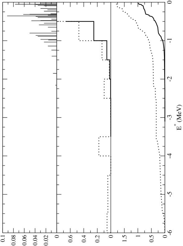
  Figure 1: Transition strength function $\left|M_{GT}(E)\right|^{2}$ assuming discrete levels for ¹³²Sn. The top graph is the discrete transition strength function. The middle graph is a histogram of the discrete function with 0.5 MeV bins, and the bottom graph is the integrated function. In the lower two graphs, the solid line corresponds to the ground-state of ¹³²Sn, and the dotted line corresponds to the first excited state.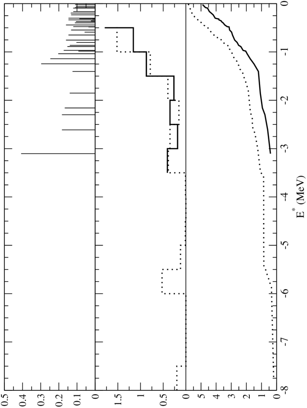

  

  Figure 2: Transition strength function $\left|M_{A}(E)\right|^{2}$ assuming discrete levels for ¹³²Sn. See Figure 1 for an explanation of the graphs.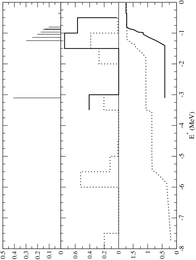

  

  Figure 3: Transition strength function $\left|M_{V}(E)\right|^{2}$ assuming discrete levels ¹³²Sn. See Figure 1 for an explanation of the graphs.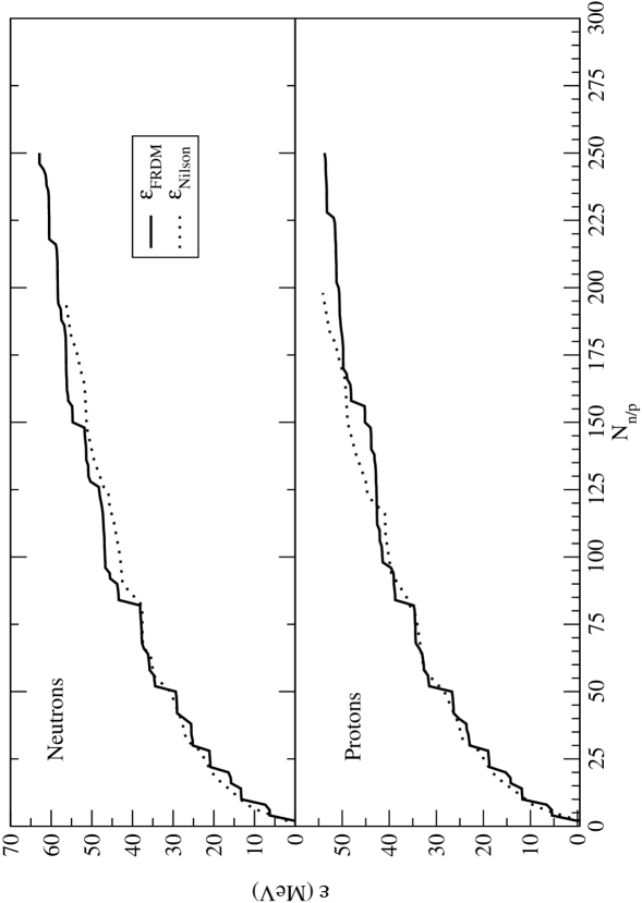

  

  Figure 4: Example of two-particle levels for ¹³²Sn neutrons (top graph) and protons (bottom graph) in the FRDM with LN pairing (solid line). The dotted line is that of the Nilsson model with no deformation.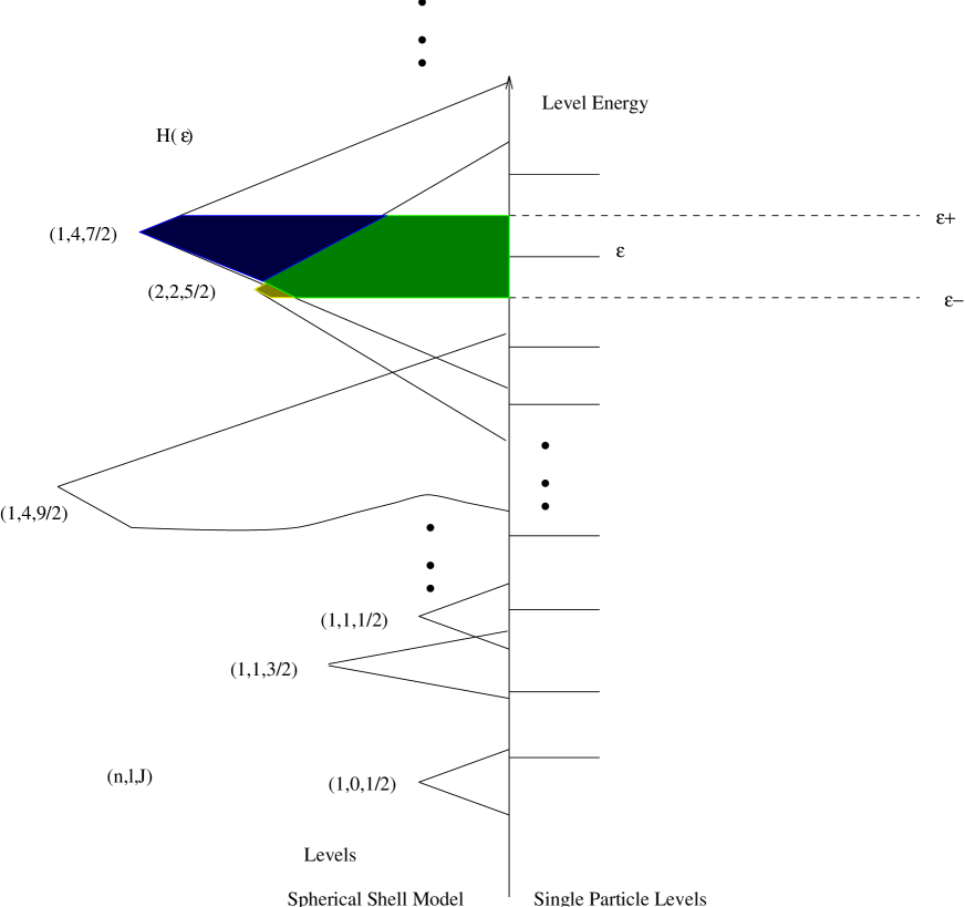

  

  Figure 5: Sample assignment of quantum numbers based on level proximity to levels of the spherical shell model [9]. For level $\varepsilon$, a contribution from two spherical shell model levels is made, and the integration is over the shaded regions in each triangular region corresponding to the level. Note that the level height corresponds to the level degeneracy, and the widths scale with standard level spacing.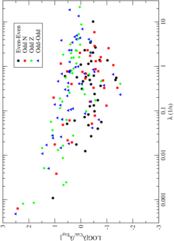

  

  Figure 6: Error in calculated $\beta$-decay rates as a function of the known half-life using the FRDM [27].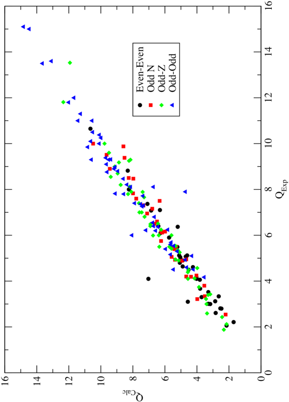

  

  Figure 7: $\beta$-Decay Q-values calculated with the FRDM compared to experimentally known Q-values.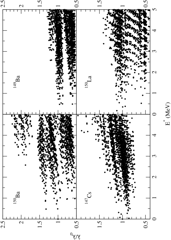

  

  Figure 8: $\beta$-Decay rates of four nuclei as a function of excited state energy of individual single-particle excitations.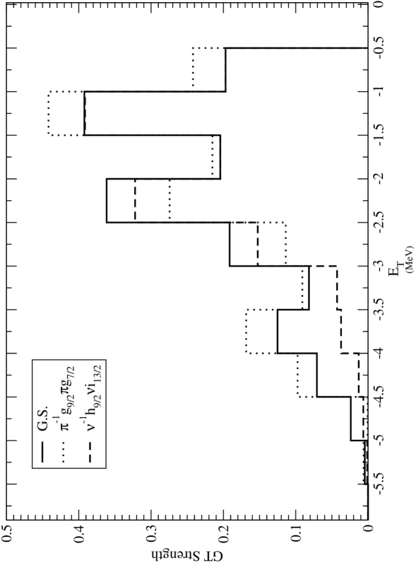

  

  Figure 9: GT transition strength function for various particle-hole states in ¹⁵⁰Ba.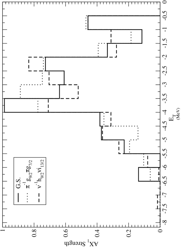

  

  Figure 10: First-forbidden transition strength function for various particle-hole states in ¹⁵⁰Ba.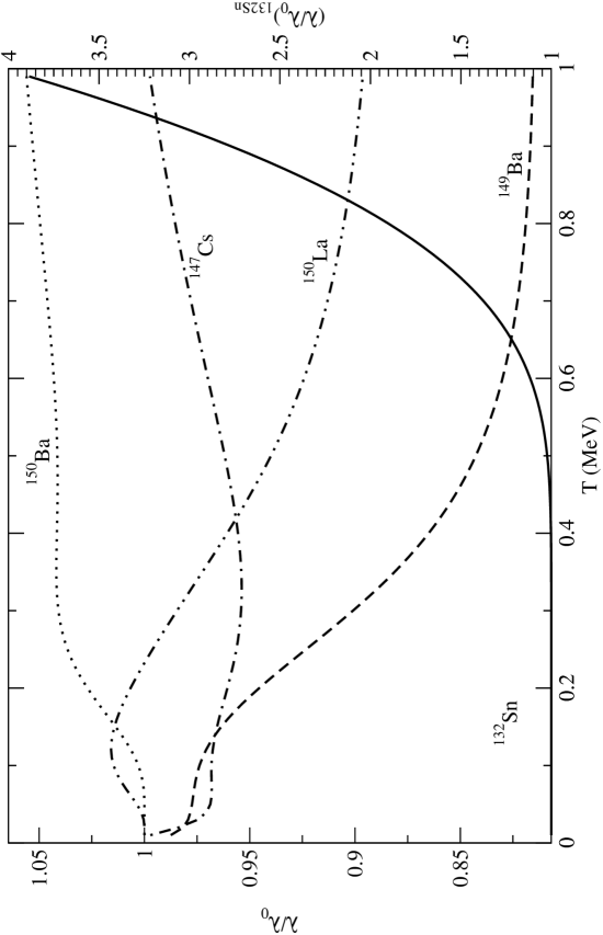

  

  Figure 11: $\beta$-Decay rates of the nuclei in Figure 8 as a function of temperature. The decay rate of ¹³²Sn is also plotted as a function of temperature.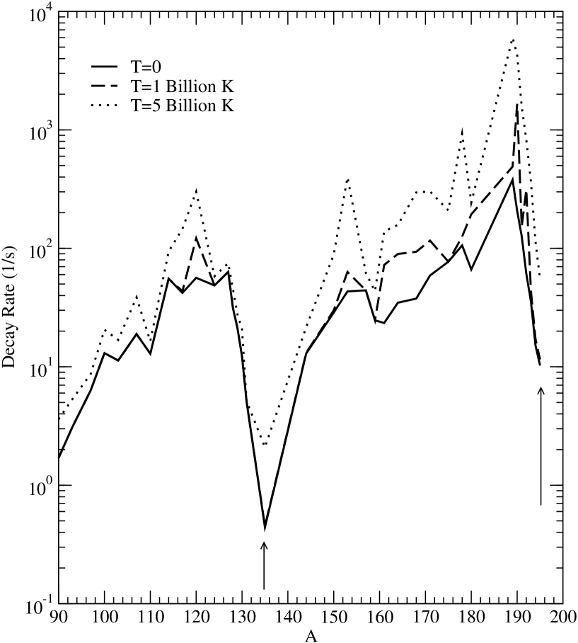

  

  Figure 12: Calculated effective $\beta$-decay rates of r-process nuclei used as a function of their mass. The nuclei represented in this figure fall along a line of neutron separation energy S_n=2.5 MeV. The arrows indicate neutron closed shells at N=82 and 126.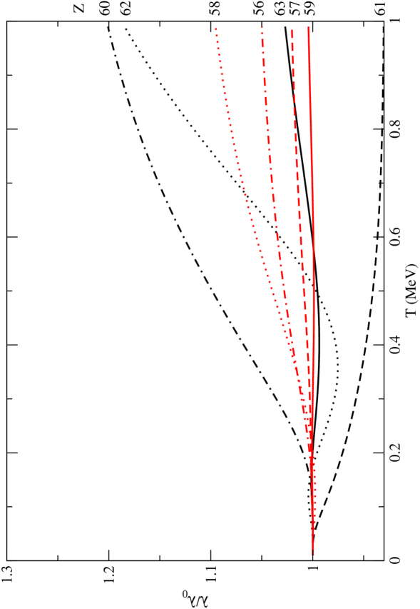

  

  Figure 13: Relative decay rates for various nuclei along the A=162 isobar as a function of temperature. In general, the nuclei closer to stability will undergo a larger increase in decay rate with temperature.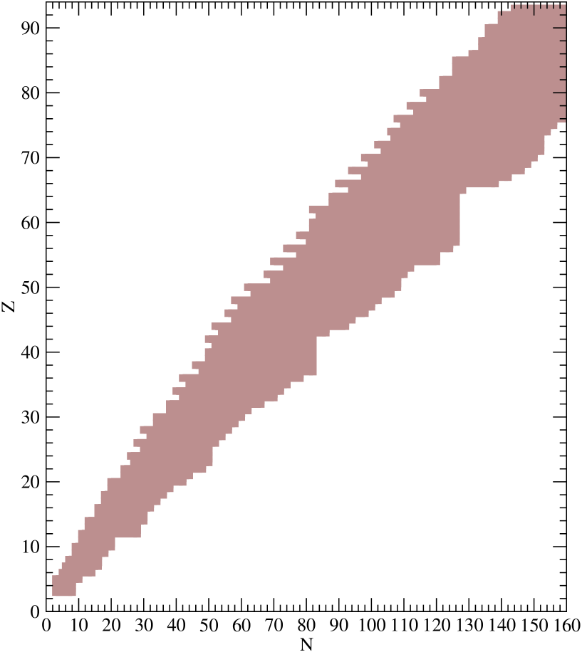

  

  Figure 14: Nuclei included in the current nuclear reaction network (Terasawa et al. 2001). Nuclei range from stable nuclei, (those on the left side of the indicated region), to those along the neutron-drip line (on the right side of the region).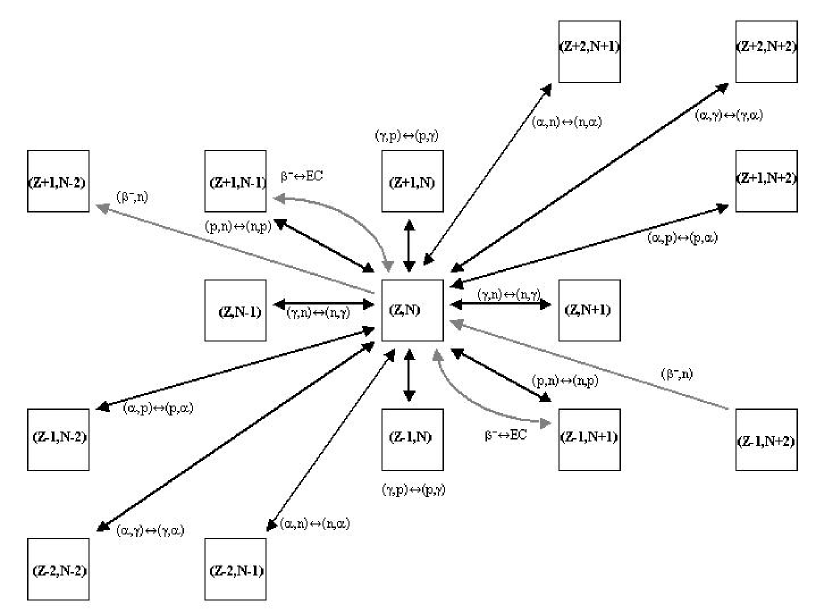

  

  Figure 15: Possible nuclear reactions included in the network calculation. Each arrow corresponds to a reaction (and its indicated inverse reaction). Not shown are neutrino interactions. Weak interactions are indicated by the lighter arrows.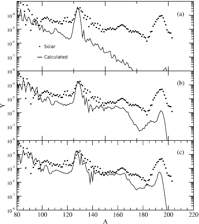

  

  Figure 16: Final r-process abundance distributions for models A, B, and C; shown in Figures (a), (b), and (c) respectively. The solar r-process abundance distribution (scaled to the figures) is given by the dots. These models do not include $\beta$-delayed neutron emission, and only include $\beta$-decays of ground-state nuclei.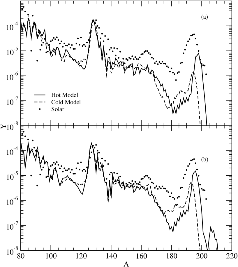

  

  Figure 17: Comparison of r-process freezeout abundance distributions for models B and C in plots (a) and (b) respectively. Solid lines and dashed curves display the calculated results with (hot model) and without (cold model) excited-state $\beta$-decays respectively. The solar distribution is also shown by the dots.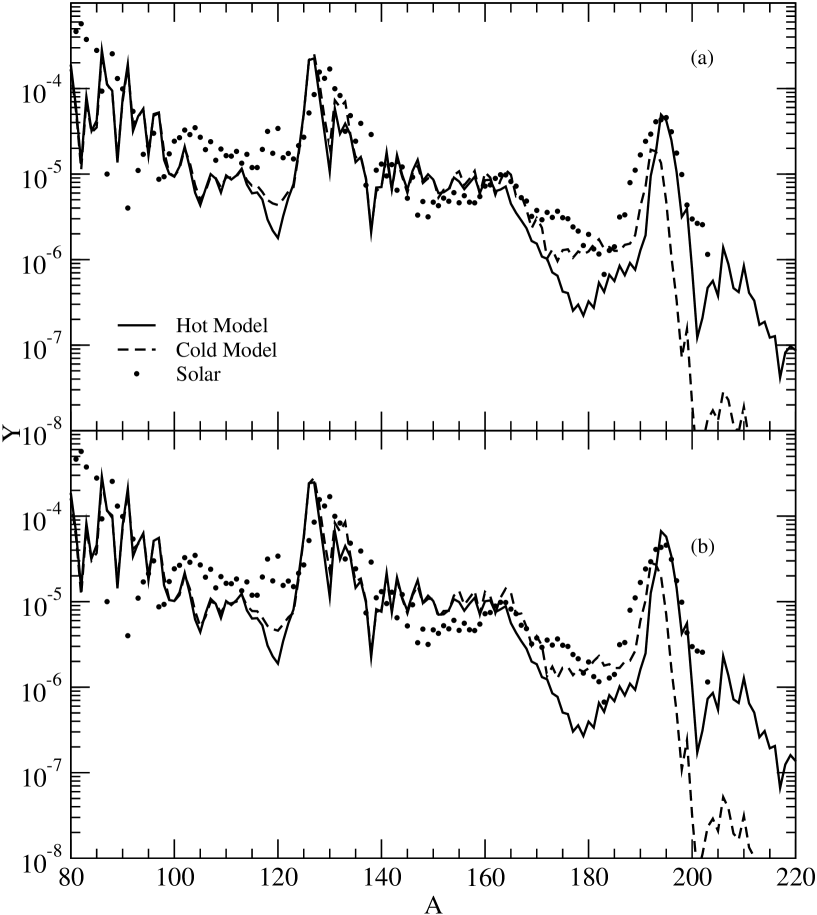

  

  Figure 18: Comparison of r-process freezeout abundance distributions for models F and G in plots (a) and (b), respectively. Solid lines and dashed curves display the calculated results with (hot model) and without (cold model) excited-state $\beta$-decays respectively. The solar distribution is also shown by the dots.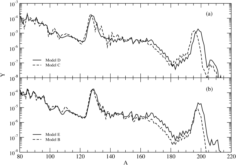

  

  Figure 19: Freezeout r-process abundance distributions for models D and C, as well as models E and B in plots (a) and (b) respectively. Both models include excited-state $\beta$-decays, while models D and E included $\beta$-delayed neutron emission.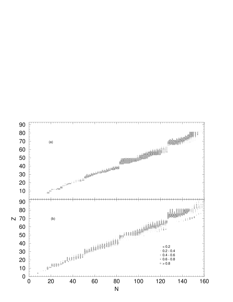

  

  Figure 20: Double and single delayed neutron emission probabilities shown in Figures (a) and (b) respectively. It can be seen that the nuclei just above the A=130 mass region have higher probabilities for two-neutron emission following $\beta$-decay.

References

- [1] Cowan J J, Thielemann F -K, and Truran J W 1990 Phys. Rep. 208 267
- [2] Wallerstein G W et al1997 Rev. Mod. Phys.69 995
- [3] Sneden C et al1998 ApJ 496 235
- [4] Cowan J J, Pfeiffer B, Kratz K -L, Thielemann F-K, Sneden C, Burles S, Tytler D, and Beers D 1999 ApJ 521 194
- [5] Qian Y Z, Vogel P and Wasserburg G J 1998 ApJ 494 285
- [6] Woosley S E et al1994 ApJ 433 229
- [7] Meyer B S 1995 ApJ 449 L55
- [8] Goriely S and Arnould M 1996 A&A 312 327
- [9] Nakata H, Tachibana T and Yamada M 1997, Nucl. Phys.A 625 521
- [10] Ichikawa S et al2005 Phys. Rev.C 71 067302
- [11] Asai M et al1999 Phys. Rev.C 59 3060
- [12] Möller P M, Pfeiffer B and Kratz K L 2003 Phys. Rev.C 67 055802
- [13] Takahashi K 1972 Prog. Theor. Phys. 47 1500
- [14] Takahashi K and Yamada M 1969 Prog. Theor. Phys. 41 1470
- [15] Takahashi K 1971 Prog. Theor. Phys. 45 1466
- [16] Nakata H, Tachibana T and Yamada M 1995 Nucl. Phys.A 95 27
- [17] Tachibana T, Yamada M and Yoshida Y 1990 Prog. Theor. Phys. 84 641
- [18] Koyama S, Takahashi K and Yamada M, 1970 Prog. Theor. Phys. 44 663
- [19] Kondoh T, Tachibana T and Yamada M 1985 Prog. Theor. Phys. 72 708
- [20] Kondoh T and Yamada M 1976 Prog. Theor. Phys. 60 136
- [21] Takahashi K, Yamada M and Kondoh T 1973 At. Data and Nucl. Data Tab. 12 101
- [22] Möller P, Nix J R and Kratz K L 1997 At. Data and Nuc. Data Tab. 66 131
- [23] Myers W D and Swiatecki W J 1974 Ann. Phys., NY84 186
- [24] Möller P M and Nix J R 1992 Nucl. Phys.A 536 20
- [25] Pradhan D G, Nogami Y and Law J 1973 Nucl. Phys.A 201 357
- [26] Shirley V S (ed) 1996 Table of Isotopes, Vol. II (John Wiley & Sons)
- [27] Möller P M et al1995 At. Data and Nucl. Data Tab. 59 185
- [28] Takahashi K, El Eid M F and Hillebrandt W 1978 A&A 67 185
- [29] Qian Y Z and Woosley S E 1996 ApJ 471 331
- [30] Shapiro S L and Teukolsky S A 1983 Black Holes, White Dwarfs, and Neutron Stars (New York: Wiley)
- [31] Otsuki K et al2000 ApJ 533 424
- [32] Wanajo S et al2001 ApJ 554 578
- [33] Wanajo S et al2007 ApJL 666 77
- [34] Teresawa M et al2001 ApJ 562 470
- [35] Teresawa M et al2004 ApJ 608 470
- [36] Tachibana T et al1988 At. Dat. Nuc. Dat. Tab. 39 251
- [37] Fuller G M and Meyer B S 1995 ApJ 453 792
- [38] Rolfs C E and Rodney W S 1988 Cauldrons in the Cosmos (Chicago, IL: The University of Chicago Press)
- [39] Surman R et al1997 Phys. Rev. Lett.79 1809
- [40] Kratz K L et al1993 ApJ 403 216
- [41] Petrasso R D et alPhys. Rev. Lett.77 2718
-
Term Description Equations N1 Number of Parent Nucleon States 1 W Weighting Function Describing 1,5 Availability of Daughter Nucleon States Energy of a Nucleon State 1-4,4,17,18,20 DΩ Transition Probability Function 1,7,9,10 Lowest Energy of a Parent Nucleon 1 Energetically Able to Decay Highest Energy of an occupied Parent Nucleon State 1-3 n3 Number of Daughter Nucleons Collected at the 3 Highest Daughter Level Due to the Pairing Force 2 Width of the Pairing Gap 2,3
Term Description Equations ni Number of Parent or Daughter Nucleons in Level i 4,5,11,12,21 Spherical Shell Model Eigenstate Mixing 6,7,11,12,20 Coefficient for Mapping to Leves in the FRDM Function for Describing Selection 7,8,11,12,21 Rules of a Transition gΩ Multiplicity Spin-Averaging Factor for 11 Transition Type Discrete Uncorrected Fermi Energy of 15,16 the kth Level dk Standard Level Density About the kth Level 15,16 H() Triangular Distribution Function Indicating 14,17,20 the Strength of the Spherical Shell Model Eigenstates q(A) Width of the Triangular Function H() 14,15 G() Sum of H() Over All Eigenstates 17,18 Integration Limits About G() and 18-20 H() for Normalizing and Determining .
Parameter Description Value Units Hydrogen atom mass excess 7.289 MeV Neutron mass excess 8.071 MeV Electronic binding constant MeV Nuclear compressibility constant 240 MeV Wigner constant 30 MeV constant 0.0 MeV Volume-energy constant 16.247 MeV Surface energy constant 22.92 MeV Curvature energy constant 0 MeV Symmetry energy constant 32.73 MeV Effective surface-stiffness constant 29.21 MeV Charge asymmetry constant 0.436 MeV Relative neutron excess - Average neutron pairing gap MeV Average proton pairing gap MeV Average neutron-proton interaction energy MeV Coulomb energy constant MeV Volume redistribution energy constant MeV Coulomb exchange constant MeV Surface redistribution energy constant MeV Form factor correction constant MeV Nuclear radius constant 1.16 fm Proton rms radius 0.80 fm Average pairing gap constant 4.80 MeV Neutron-proton interaction constant 6.6 MeV Diffuseness of Yukawa function 0.70 fm LN pairing constant 3.2 MeV
Parameter Region Label A C D E F 67N75 1 - - - 0 - 1 0 0.03 76N77 2 2 2 2.5 0.3 1 0 - - N=78 3 3 9 0.25 0.095 1 0 - - N=79 4 1.25 5 0.5 0.2 1 0 - - 80N81 5 - - - 0 - 1 0 0.018 N=82 6 - - - 0 - 1 0.032 0.045 39Z42 7a - - - 0 - 1 0 47Z51 43Z46 7b 9 1 2.5 0.2 1 0 - - 82N126 52Z54 7c 12 1 4 0.28 1 0 - - Z=55 7d - - - 0 - 1 0.08 0.025 Z56 7e 12 8 0.5 0.04 1 0 - - N=126 8 4 1.2 0.3 1 0 - - 60Z63 9a 5 3 0.75 0.25 1 0 - - 64Z66 9b 20 0.88 7.3 1 0 0 - - N126 68Z71 Z=67 9c 1.5 5 0.25 0.4 1 0 - - 72Z74 9d - - - 0 - 1 0.3 0.025 Table 5: Parameters Used in the Supernova Model -
Model M/M⊙ R(km) Lν (1052erg s-1) Ye (,n)? (s) S (k) A 1.7 10 0.7 0.4 N 0.017 110 B 2 10 0.7 0.4 N 0.014 151 C 2 10 0.5 0.4 N 0.021 162 D 2 10 0.5 0.4 Y 0.021 162 E 2 10 0.7 0.4 Y 0.014 151 F 2 10 0.5 0.37 Y 0.021 162 G 2 10 0.5 0.35 Y 0.021 162