The Spin-1 Heisenberg Antiferromagnet: New Results from Series Expansions

Abstract

We calculate ground state properties (energy, magnetization, susceptibility) and one-particle spectra for the $S=1$ Heisenberg antiferromagnet with easy-axis or easy-plane single site anisotropy, on the square lattice. Series expansions are used, in each of three phases of the system, to obtain systematic and accurate results. The location of the quantum phase transition in the easy-plane sector is determined. The results are compared with spin-wave theory.

I Introduction

Magnetic materials with S = 1 ions have been of interest for many years. The ‘classic’ 2-dimensional Heisenberg antiferromagnet K₂NiF₄ was studied in the 1970s birgeneau1970 . In the 1980s a number of (weakly coupled) linear chain systems were investigated, including CsNiCl₃ steiner1987 , which has a weak axial anisotropy, CsFeBr₃ dorner1988 , which has strong planar anisotropy, and the complex materials NENP (Ni(C₂H₈N₂)₂NO₂(ClO₄)) renard1988 and NENC (Ni(C₂H₈N₂)₂Ni(CN₄)) orendac1995 , which have weak and strong planar anisotropy, respectively. The spin gaps observed in the weakly anisotropic materials steiner1987 ; renard1988 are believed to be examples of the behaviour predicted by Haldane haldane1983 . More recent work includes molecular oxygen adsorbed on graphite murakami1996 , the bilayer material Ba₃Mn₂O₈ uchida2002 ; stone2008 , a new spin gapped material NiGa₂S₄ nakatsuji2005 , which, it has been argued tsunetsugu2006 ; bhattacharjee2006 , may be a ‘spin nematic’ chandra1991 , and a system of spin-1 bosonic atoms in an optical lattice greiner2002 .

We have previously used series expansion methods to study a wide range of spin-1/2 quantum antiferromagnets oitmaa2006 . Quantum fluctuations will be reduced when S = 1, but new physical features are possible. Besides the gapped Haldane phase in 1-dimensional systems haldane1983 , additional terms, such as biquadratic exchange and/or single site anisotropy, which are absent in spin-1/2 systems, can lead to quadrupolar/nematic phases with long range order but no magnetic moment, novel quantum phase transitions sachdev1999 , and richer excitation spectra. We explore some of these issues in the present work, within the context of the Hamiltonian

$$H=J\sum_{<ij>}{\bf S_{i}\cdot S_{j}}-D\sum_{i}(S_{i}^{z})^{2}$$ (1)

which describes a Heisenberg antiferromagnet ($J>0$) with isotropic exchange and a single ion anisotropy which gives rise to an easy axis ($D>0$) or easy plane ($D<0$).

A significant single ion anisotropy is believed to be present in many of the 1-dimensional materials referred to above, and has been included in analyses of the experimental data. Consequently there has been much theoretical work devoted to the Hamiltonian (1) on a linear chain golinelli1992 ; papanicolaou1990 ; chen2003 . For higher dimensions various approaches have been used, including mean-field type theories devlin1971 ; khajehpour1975 , spin wave approximations rastelli1974 ; lindgard1975 and a coupled cluster calculation wong1994 . We will compare our results with each of these, where possible.

Figure 1: The phase diagram of the spin-1 J-D model on the square lattice at zero temperature, showing the Ising antiferromagnetic phase (IAFM), planar antiferromagnetic phase (PAFM), and quantum paramagnetic phase (QPM).

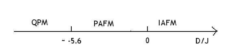
The present work deals with the 2-dimensional square (SQ) lattice. For D = 0 the spin-1 system has Néel order at zero temperature neves1986 , with quantum fluctuations reducing the staggered magnetization by some 20% singh1990 . When $D>0$ the system will order along $z$, the ‘easy axis’. The order parameter will be ‘Ising-like’ and long-range order will persist at finite temperature, up to a critical line $T_{c}(D)$ with Ising (n=1) exponents. For $D<0$, on the other hand, the z-axis is a ‘hard’ direction and the spins will order antiferromagnetically along some direction in the x-y plane (at least for small $|D|$). The order parameter has n=2 components and the continuous symmetry will be spontaneously broken. Long-range magnetic order will not persist to finite temperature (the Mermin-Wagner theorem) although one may expect a Kosterlitz-Thouless transition. For large negative D the physics will be quite different. In the limit $D\rightarrow-\infty$ the ground state will be a simple product state with $S^{z}=0$ at all sites. This is a quadrupole state with no magnetic order. Thus we expect a quantum phase transition at some $D=D_{c}$, which we will locate using our series approach. The phase diagram is illustrated in Figure 1.

It is also of interest to study the elementary excitations above the ground state. For D = 0 these are magnons, with Goldstone modes at ${\bf k}=(0,0)$ and $(\pi,\pi)$. A gap will open in the spectrum for small positive D, which will be proportional to $\sqrt{D}$, according to spin-wave theory. On the other hand for large $|D|$ the picture will be quite different. For large negative D the excitations will consist of isolated $S^{z}=\pm 1$ spins, which have been termed excitons and anti-excitons papanicolaou1990 . These will have an energy gap, which we expect will vanish as $D\rightarrow D_{c}-$. For large positive D an excitation with $\Delta S^{z}=2$ (i.e. $S^{z}=-1\leftrightarrow S^{z}=+1$) will have a smaller energy than a single magnon. We expect, and confirm below, that there is a 2-magnon bound state, and we calculate its dispersion curve.

To conclude this Introduction we will briefly describe the series expansion approach, for both ground state bulk properties and excitations, referring the reader to our recent book oitmaa2006 for further details. The approach is based on writing the Hamiltonian in the usual perturbative form

$$H=H_{0}+\lambda V$$ (2)

where $H_{0}$ has a simple known ground state. This subdivision is carried out in various ways, appropriate to the different phases of the model. Series are derived for the ground state energy, order parameter and other quantities of interest, in powers of $\lambda$, and extrapolated to $\lambda=1$ by numerical methods (Padé approximants or integrated differential approximants). Calculations are carried out for a sequence of finite connected clusters, and the results combined to obtain bulk lattice properties.

A similar approach is used for excitations. An orthogonal transformation is used to obtain an ‘effective Hamiltonian’ matrix for each cluster, yielding transition amplitudes for the excitation in real space, which are then combined to obtain dispersion curves throughout the Brillouin zone. Points where the gap approaches zero can be easily identified, and corresponding series obtained for the gap itself.

In the body of the paper we will present and analyse various results in the easy-axis ($D>0$) phase (Section II), and in the easy-plane ($D<0$) phase (Section III). Section IV contains a summary and conclusions.

II The Easy Axis ($D>0$) Case

II.1 Bulk Ground State Properties

Figure 2: Ground state energy per spin for the easy-axis J-D model on the SQ lattice. The individual points are the estimates from series . The various lines are results of different spin-wave approximations: SW1, short-dashed line; SW1a, long-dashed line; SW2, solid line. For convenience, we plot $E_{0}+D$ versus $D$, and set $J=1$.

We have computed series for the ground state energy per spin and for the ground state staggered magnetization to order $\lambda^{12}$, where $H_{0}$ and $V$ are

$$H_{0} = J\sum_{<ij>}S^{z}_{i}S^{z}_{j}-D\sum_{i}(S^{z}_{i})^{2}-h\sum_{i}\eta_{i}S^{z}_{i}$$ (3)

$$V = \frac{1}{2}\sum_{<ij>}(S^{+}_{i}S^{-}_{j}+S^{-}_{i}S^{+}_{j})$$ (4)

for various values of D. Here $h$ is a staggered field, included to allow calculation of the order parameter, and $\eta_{i}=\pm 1$ on the respective sublattices. We do not present the series coefficients here, but can provide them on request.

Figures 2 and 3 show the ground state energy and staggered magnetization versus D.

Figure 3: Staggered magnetization for the easy-axis J-D model on the SQ lattice. Notation as in Figure 2.

For purposes of comparison, we also present results from conventional spin-wave theory, first order spin wave theory (SW1), modified first-order theory (SW1a) and second order theory (SW2). The first order theory gives

$$E_{0} = -4J-(1+\eta)D+\frac{1}{N}\sum_{k}\epsilon_{k}$$ (5)

$$M_{s} = \frac{3}{2}-\frac{1}{N}\sum_{k}\frac{4J+2\eta D}{\epsilon_{k}}$$ (6)

where $\epsilon_{k}$, the spin-wave energy, is given by

$$\epsilon_{k}=4J\sqrt{(1+\eta D/(2J))^{2}-\gamma_{k}^{2}}$$ (7)

with $\gamma_{k}=(\cos k_{x}+\cos k_{y})/2$. The constant $\eta=1,1/2$ for SW1, SW1a respectively. This factor arises from a choice in treating the anisotropy term. In large S theory $\eta=1$ but for $S=1$, as here, normal ordering of the quartic boson terms gives $\eta=1/2$. This is explained in Appendix A, where we also present the more complex second-order theory.

As is apparent from Figure 2, SW1 is a rather poor approximation, but SW1a and SW2 are in almost quantitative agreement with the series results, within 1%. For the magnetization, a simlar conclusion applies. Note that the magnetization exhibits a square-root cusp behaviour near $D=0$, in agreement with the spin-wave theory.

II.2 1-Magnon Excitations

At least for small D the lowest energy excitations, in the unperturbed system, consist of a single spin excited from its ordered $S^{z}=\pm 1$ state to $S^{z}=0$, i.e. $\Delta S^{z}=\pm 1$. The quantum fluctuations, embodied in the perturbation V, will then allow this to propagate through the lattice, forming a coherent magnon band.

Within spin wave theory the excitation energy is given by equation (7) (or the more general result in Appendix A). We have computed a series expansion for the excitation energy to order $\lambda^{11}$, following the original work of Gelfand gelfand1996 (see also ref. 13).

In Figure 4 we show the excitation energy, along symmetry lines in the Brillouin zone, for the case $D/J=1$, and again for comparison the spin-wave results. Again we see that SW1 is a rather poor approximation, but SW1a and SW2 provide an excellent description of the data, with SW1a actually better than SW2.

Figure 4: Single-magnon excitation energy at D/J = 1.0 along symmetry lines in the Brillouin zone, obtained from series (full dots) and spin wave approximations. Notation as in Figure 2.

The dispersion curves are smooth and rather featureless. The most significant feature is the opening of a gap at ${\bf k}=(0,0)$ for any non-zero D. This reflects, in the easy axis case, the fact that the remnant O(2) symmetry of the Hamiltonian is not spontaneously broken in this case, and so Goldstone modes are absent.

Figure 5 shows the dependence of the gap at ${\bf k}=(0,0)$ on the coupling D. The $\sqrt{D}$ dependence at small D predicted by spin wave theory is clearly evident. At large D the single-magnon gap is predicted to increase linearly with D.

Figure 5: Single-magnon excitation energy at ${\bf k}=(0,0)$ as a function of $D$ in the easy-axis region (setting $J=1$). The solid line is the second order spin wave approximation (SW2).

II.3 Large D Excitations

It is clear that for large D the single-magnon excitations of the previous subsection will not be the lowest energy excitations of the system. Their energy will be of order D, whereas an excitation with $\Delta S^{z}=2$ will have an energy of order J. Such an excitation, created at a particular site, can again propagate through the lattice, forming a quasiparticle band. We may think of this as a two-magnon bound state where the magnons are bound on the same site (see Appendix A).

Figure 6 shows the dispersion relation for the $\Delta S^{z}=2$ excitation at $D/J=1$ compared with the lower edge of the two-magnon continuum. It can be seen that in the mid-region of the plot the excitation indeed seems to lie below the continuum, becoming a bound state at slightly below this coupling. The energy here is close to the asymptotic limit of 8 units. In the wings of the plot the error bars are much larger, and the excitation may not be bound: it is possible that these facts may be related, At higher values of $D/J$, the bound state energy remains close to 8 units, so that the binding energy rises almost linearly with $D/J$.

Figure 6: Dispersion relation of the $\Delta S^{z}=2$ excitation at $D/J=1.0$. The points with error bars are the series estimates. The dashed line is the lower limit of the 2-magnon continuum.

II.4 Finite Temperature Phase Transition

Since the continuous O(3) symmetry of the Heisenberg model is destroyed by an easy-axis anisotropy term, and the order parameter is Ising-like, taking one of two possible values, the ordered ground state will persist to finite temperature, up to a critical temperature $T_{c}(D)$. We have derived high-temperature series in the variable $K=J/k_{B}T$ to order $K^{11}$ for the staggered susceptibility $\chi_{s}$, for various values of D. These are then analysed via standard Dlog Padé approximants to obtain the critical temperature and exponent. Figure 7 shows the critical temperature versus D and, for comparison, the mean field result khajehpour1975 . One would not expect MFA to give accurate results in 2 dimensions, and indeed there is a sizeable discrepancy. We note that MFA gives a finite critical temperature even for the isotropic case, $D=0$, which violates the Mermin-Wagner theorem. The critical exponent $\gamma$ is consistent with the universal 2D Ising exponent 7/4, although there is substantial scatter in the estimates from these relatively short series.

Figure 7: Critical temperature versus $D/J$ for the $S=1$ easy-axis model on the SQ lattice. The filled circles are the series results, with estimated errors no larger than the size of the symbols. The line is a guide to the eye. The dashed line is the MFA result khajehpour1975 .

III The Easy-Plane ($D<0$) Case

The easy-plane case shows much more interesting physics, including, as we shall see, two distinct phases separated by a quantum phase transition (QPT).

For small $|D|$ the spins will be preferentially in the x-y plane (choosing z as the hard axis) and the Hamiltonian will have O(2) symmetry. At T = 0 this symmetry will be spontaneously broken and the system will exhibit Néel order in some direction, reduced by quantum fluctuations. We refer to this as the planar antiferromagnetic phase (PAFM). The broken O(2) symmetry will result in a single gapless Goldstone mode. In the following we will present results from series expansions for both ground state bulk properties and for single-magnon excitations. These will again be compared with spin wave theory. Although there will be no ordered phase at finite temperature we expect a finite temperature Kosterlitz-Thouless transition. However we do not explore this aspect.

For large $|D|$, where the anisotropy term is dominant, we expect the system to prefer a singlet phase where spins are in the $S^{z}=0$ state. This phase has no magnetic order, and is aptly referred to as a quantum paramagnetic phase (QPM). Quantum fluctuations, arising from the exchange terms, will modify the state. Low energy excitations in the QPM phase consist of spins excited to the $S^{z}=\pm 1$ states, which have been termed ‘excitons’ and ‘anti-excitons’. In the following we derive series for both bulk properties and excitations in the QPM phase. An analytic approximation, due to Papanicolaou papanicolaou1990 , is also presented and compared with the series results.

As $|D|$ is reduced in the QPM phase (or increased in the PAFM phase) a quantum phase transition is found to occur and we use series expansions to locate this transition accurately, and to study its properties.

III.1 PAFM Phase: Bulk Ground State Properties

Figure 8: Ground state energy per site in the easy-plane region for the $S=1$ J-D model on the SQ lattice. The squares are series results for the PAFM phase, and the the dashed line is the first order spin wave estimate in the PAFM phase. We have set $J=1$.

It is convenient to rotate the spin axes and to write the Hamiltonian as

$$H = J\sum_{<ij>}(S^{z}_{i}S^{z}_{j}+S^{x}_{i}S^{x}_{j}+S^{y}_{i}S^{y}_{j})-D\sum_{i}(S^{x}_{i})^{2}$$ (8)

$$= J\sum_{<ij>}S^{z}_{i}S^{z}_{j}+\frac{1}{2}J\sum_{<ij>}(S^{+}_{i}S^{-}_{j}+S^{-}_{i}S^{+}_{j})$$

$$-\frac{1}{4}D\sum_{i}(S^{+}_{i}+S^{-}_{i})^{2}$$

where z is the ordering axis and x is the hard axis. We now decompose $H=H_{0}+\lambda V$, with

$$H_{0} = J\sum_{<ij>}S^{z}_{i}S^{z}_{j}+\frac{1}{2}D\sum_{i}(S^{z}_{i})^{2}-h\sum_{i}\eta_{i}S^{z}_{i}$$ (9)

$$V = \frac{1}{2}J\sum_{<ij>}(S^{+}_{i}S^{-}_{j}+S^{-}_{i}S^{+}_{j})$$ (10)

$$-\frac{1}{4}D\sum_{i}(S^{+}_{i}S^{+}_{i}+S^{-}_{i}S^{-}_{i})$$

where we have dropped a constant term $-ND$ and, as before, included a staggered field term.

We have computed series for the ground state energy and staggered magnetization to order $\lambda^{12}$. Figures 8 and 9 show the ground state energy and magnetization versus D, as obtained by analysis of these series.

Figure 9: Staggered magnetization in the PAFM phase of the $S=1$ J-D model on the SQ lattice. The points are series estimates, and the short-dashed line is first order spin wave theory. The long-dashed line is a fit in the critical region.

For comparison we show the results of first order spin wave theory (SW1). The details of this are given in Appendix B. In Figure 8, we see that the SW1 theory gives quite a good description of the bulk ground state energy in the PAFM phase, as compared with the series estimates (squares).

The series estimates for the magnetization in the PAFM phase were obtained as follows. The perturbation series in $\lambda$ typically exhibit a singularity of form $(\lambda_{c}-\lambda)^{\sigma}$ for $\lambda_{c}$ only a little larger than $1$, so a naive Padé extrapolation in $\lambda$ gives unreliable results. Instead, at each value of $D/J$ we estimate $\lambda_{c}$ and $\sigma$ using standard Dlog Padé methods, and then extrapolate the series to $\lambda=1$ using a variable $\delta=1-(1-\lambda/\lambda_{c})^{\sigma}$. The data seem to show a crossover from a singularity with very small $\sigma$ at small negative $D$, to another one with $\sigma\simeq 0.27$ nearer the critical point. The estimated magnetization at the crossover point, around $D/J=-3.5$, shows large error bars.

The results are shown in Figure 9. We note that SW1 gives qualitatively the right behaviour at small $|D|$, but becomes rather poor for large $|D|$, where it shows no sign of the decrease towards the transition point. Near $D=0$, the magnetization shows a square-root cusp, the mirror of that in the easy-axis region, marking the transition from the easy-axis to the easy-plane phase. The series results show a rapid decrease in magnetization beyond $D/J\sim-5$, heralding the expected quantum phase transition to the QPM phase. However the error bars are large and it is not possible to locate the transition with any degree of precision from the magnetization alone. The fit in this region will be discussed in Section III.4.

III.2 PAFM Phase: Elementary Excitations

Figure 10: Single-magnon dispersion curves for the PAFM phase for $D/J=-1.0$ (circles) and $D/J=-5.0$ (squares) The dashed lines are from the first order spin wave theory.

We have computed series for the single-magnon excitations in the PAFM phase, to order $\lambda^{10}$. The series are analysed to compute the magnon energies $\epsilon({\bf k})$, and these are shown in Figure 10, along symmetry lines in the Brillouin zone, for values $D/J=-1.0$ and $-5.0$. Again, for comparison, we show the result of first order spin wave theory (Appendix B). We note that spin fluctuations transverse to the ordering direction are no longer isotropic, and hence the full Brillouin zone must be used.

The energy gap vanishes at ${\bf k}=(\pi,\pi)$, according to spin-wave theory, corresponding to the expected Goldstone mode. The series extrapolations in $\lambda$ by means of standard Padé approximants still give a finite result at that point, because they assume the series is regular at $\lambda=1$. The energy gap at ${\bf k}=(0,0)$ is indeed finite, and behaves like $\sqrt{D}$ at small $|D|$, mirroring that in the easy-axis region. It rises rapidly at large $D$. The qualitative behaviour is well reproduced by SW1 theory.

III.3 QPM Phase: Bulk Ground State Properties

To investigate the large $|D|$ quantum paramagnetic phase we decompose the full Hamiltonian as $H=H_{0}+\lambda V$, with

$$H_{0}=|D|\sum_{i}(S^{z}_{i})^{2}+J\sum_{<ij>}S^{z}_{i}S^{z}_{j}$$ (11)

and

$$V=\frac{1}{2}\sum_{<ij>}(S^{+}_{i}S^{-}_{j}+S^{-}_{i}S^{+}_{j})$$ (12)

The unperturbed ground state has all spins in the $S^{z}=0$ state, and the effect of the perturbation is to create (+ -) states on neighbouring sites (exciton-antiexciton pairs). Note that, unlike the previous sections, we do not perform a spin rotation on one sublattice. The derivation then follows standard lines, and we have obtained series to order $\lambda^{12}$ for both the ground state energy and for the ‘quadrupole moment’ $Q=<3(S^{z}_{i})^{2}-2>$. An alternative approach, in which only the anisotropy term is included in $H_{0}$ and the full exchange term as $V$, is also possible. The expansion parameter is then $J/D$. We have carried this through but it seems not to yield any improvement in precision.

Figure 11: Ground state energy per site at negative $D/J$ (setting $J=1$). The open circles are estimates in the QPM phase, and the filled squares are PAFM estimates.

In Fig. 11 we plot the ground state energy versus $D/J$ in the QPM phase. We also include some of the data from the PAFM expansion (Section III.1, above) near the crossover region. As can be seen, the two curves meet smoothly, but the precision is inadequate to distinguish between a second order transition or a weak first order transition (with a small discontinuity in slope). The quadrupole moment $Q$ increases smoothly from a value $-2$ at large $|D|$ to approximately $-1.6$ at $D=-5$, but shows no interesting behaviour.

III.4 QPM Phase: Excitations

Figure 12: Single particle dispersion in the QPM phase along symmetry lines in the Brillouin zone, for $D/J=-10.0$ (circles) and $D/J=-6.0$ (squares).

Figure 13: The energy gap $\epsilon({\bf k})$ at momentum ${\bf k}=(\pi,\pi)$ in the QPM phase, as a function of $D$ ($J=1$). The dashed line is a fit to the data in the region $-7.0<D/J<-5.6$, in the neighbourhood of the critical point.

The low energy excitations, termed ‘excitons’ and ‘antiexcitons’, arise from exciting one of the $S^{z}=0$ sites to $S^{z}=\pm 1$. Such a local excitation can then propagate through the lattice as a well defined quasiparticle with energy $\epsilon({\bf k})$.

Using the Hamiltonian decomposition (11,12) and the usual linked cluster methods, we have computed series for the excitation energy to order $\lambda^{10}$. Figure 12 shows a plot along symmetry lines in the Brillouin zone for two values of $D/J$, viz. $D/J=-10.0,-6.0$. As is apparent, the energy gap at $(\pi,\pi)$ is closing as $D$ increases, and we expect it to vanish at the quantum phase transition point $D_{c}$. We found that the best way of locating the phase transition from the QPM to the PAFM phase was to perform a Dlog Padé analysis of the series in $\lambda$ for the energy gap in the QPM phase at ${\bf k}=(\pi,\pi)$, looking for the zero point. Hence we estimate the critical point, where the energy gap goes to zero at the physical value $\lambda=1$, lies at $(D/J)_{c}=-5.61(5)$. A similar analysis of the magnetization in the PAFM phase gives a somewhat less reliable estimate, $(D/J)_{c}=-5.7(2)$, which is compatible with the figure above. We note that the coupled cluster calculation wong1994 gives $(D/J)_{c}=-6.97,-6.38$ at successive levels.

The energy gap in the QPM at momentum ${\bf k}=(\pi,\pi)$ was again estimated by forming Padé approximants in the variable $\delta=1-(1-\lambda/\lambda_{c})^{\sigma}$, where $\lambda_{c}$ and $\sigma$ are the location and critical index, respectively, of the energy gap as a function of $\lambda$, estimated by the usual Dlog Padé methods. The index $\sigma$ appeared consistently as $0.70(2)$.

Figure 13 shows the resulting estimates of the energy gap in the QPM at this momentum, as a function of $D/J$, with a fit near the critical region of the form $\epsilon({\bf k})\propto(5.61-D/J)^{\nu}$, where the fit gives $\nu=0.73(3)$. One would naturally conclude that the critical indices $\nu$ and $\sigma$ are identical.

A similar fit of the form $M_{s}\propto(5.61+D/J)^{\beta}$ to the magnetization in the PAFM phase is shown in Figure 9. The fit over the range $-5.6<D/J<-4.5$ gives $\beta=0.25(3)$, and again one would conclude that the magnetization indices in the variables $\lambda$ and $D/J$ are the same.

These indices should be compared with the expected values for the universality class corresponding to this quantum phase transition, namely those of the classical O(2) model in three dimensions, which are $\nu=0.671$, $\beta=0.346$ guida1998 . The agreement is not very good, but this is perhaps not surprising in view of the crude and indirect methods used in our estimates.

An analytic theory for the QPM phase has been proposed by Papanicolaou papanicolaou1985 , based on a generalized Holstein-Primakoff transformation. This gives

$$\epsilon({\bf k})=\sqrt{D(D+8J\gamma_{{\bf k}})}$$ (13)

which yields for the $(\pi,\pi)$ gap

$$\epsilon(\pi,\pi)=\sqrt{D(D+8J)}$$ (14)

i.e. $(D/J)_{c}=-8.0$, $\nu=0.5$. These do not agree well with the series estimates.

IV Conclusions

Magnetic systems with $S=1$ and with easy-axis or easy-plane crystal field anisotropy have become of interest again, as a result of new materials and suggestions of novel quantum phases. Early theoretical approaches, based on mean field, Green’s function, and spin-wave approximations are of uncertain and dubious validity. Present day (numerical) approaches such as Quantum Monte Carlo and series methods allow rather precise calculation of ground state properties and of the spectrum of elementary excitations, and hence of energy gaps.

We have used comprehensive series methods, for the first time, to study the model on the square lattice. Three distinct phases are identified, in agreement with previous work. We have compared our results with those of first and second order spin-wave theory. In the Ising antiferromagnetic (IAFM) phase, the first order theory deviates substantially from the series results, but the second order theory (and even a ’modified’ first order theory) are in quantitative agreement with series, within one or two percent. In the planar antiferromagnetic (PAFM) phase, only a first order theory is available, which gives a reasonable description at small negative $D$, but fails in the neighbourhood of the transition to the quantum paramagnetic (QPM) phase.

The transition between the planar antiferromagnetic and quantum paramagnetic phase is located at $D/J=-5.61(5)$. The transition appears to be of second order, with critical indices in qualitative but not quantitative agreement with those of the classical O(2) model in three spatial dimensions. We would not claim any contradiction here as the error bars on our estimates are rather large.

The series approach followed in this paper can, of course, be applied equally well to other lattices. Indeed there is considerable interest in the one-dimensional case, and work on this is in progress.

Appendix A Spin Wave Theory for the Easy-Axis ($D>0$) Case

The spin-wave approximation is well known. Nevertheless, for completeness, we give a brief summary of the second order theory for this model, following closely the treatment of ref. zheng1991 .

The initial Hamiltonian

$$H=J\sum_{<ij>}[S^{z}_{i}S^{z}_{j}+\frac{1}{2}(S^{+}_{i}S^{-}_{j}+S^{-}_{i}S^{+}_{j})]-D\sum_{i}(S^{z}_{i})^{2}$$ (15)

is expressed in terms of boson operators $a_{i},b_{j}$ on the respective sublattices via a Dyson-Maleev transformation

$$\begin{array}[]{ccc}A:\hskip 14.22636ptS^{z}_{i}=S-a^{\dagger}_{i}a_{i},&S^{+}_{i}=\sqrt{2S}(1-a^{\dagger}_{i}a_{i}/2S)a_{i},&S^{-}_{i}=\sqrt{2S}a^{\dagger}_{i}\\ B:\hskip 14.22636ptS^{z}_{j}=b^{\dagger}_{j}b_{j}-S,&S^{+}_{j}=\sqrt{2S}b^{\dagger}_{j}(1-b^{\dagger}_{j}b_{j}/{2S}),&S^{-}_{j}=\sqrt{2S}b_{j}\end{array}$$ (18)

followed by a transformation to k-space (Bloch) operators

$$a_{i}=\sqrt{\frac{2}{N}}\sum_{{\bf k}}e^{-i{\bf k\cdot R_{i}}}a_{\bf k},\hskip 14.22636ptb_{j}=\sqrt{\frac{2}{N}}\sum_{{\bf k}}e^{i{\bf k.R_{j}}}b_{{\bf k}}$$ (19)

where the sum is over N/2 points in the reduced Brillouin zone, giving

$$H = -\frac{1}{2}NS^{2}(zJ+2D)+[S(zJ+2D)-D]\sum_{\bf k}(a^{\dagger}_{\bf k}a_{\bf k}+b^{\dagger}_{\bf k}b_{\bf k})+zJS\sum_{\bf k}\gamma_{\bf k}(a^{\dagger}_{\bf k}b^{\dagger}_{\bf k}+a_{\bf k}b_{\bf k})$$ (20)

$$-\frac{zJ}{N}\sum_{{\bf k_{1},k_{2},k_{3},k_{4}}}\Delta({\bf k_{1}-k_{2}-k_{3}+k_{4}})[2\gamma_{{\bf k_{3}-k_{4}}}a^{\dagger}_{{\bf k_{1}}}a_{{\bf k_{2}}}b^{\dagger}_{{\bf k_{3}}}b_{{\bf k_{4}}}+\gamma_{{\bf k_{4}}}a^{\dagger}_{{\bf k_{1}}}a_{{\bf k_{2}}}a_{{\bf k_{3}}}b_{{\bf k_{4}}}+\gamma_{{\bf k_{1}}}a^{\dagger}_{{\bf k_{1}}}b^{\dagger}_{{\bf k_{2}}}b^{\dagger}_{{\bf k_{3}}}b_{{\bf k_{4}}}]$$

$$-\frac{2D}{N}\sum_{{\bf k_{1},k_{2},k_{3},k_{4}}}\delta({{\bf k_{1}+k_{2}-k_{3}-k_{4}}})[a^{\dagger}_{{\bf k_{1}}}a^{\dagger}_{{\bf k_{2}}}a_{{\bf k_{3}}}a_{{\bf k_{4}}}+b^{\dagger}_{{\bf k_{1}}}b^{\dagger}_{{\bf k_{2}}}b_{{\bf k_{3}}}b_{{\bf k_{4}}}]$$

Here $z$ is the coordination number of the lattice and $\gamma_{{\bf k}}$ is the usual

$$\gamma_{{\bf k}}=1/z\sum_{nn}\exp{i{\bf k\cdot\delta}}=\frac{1}{2}(\cos k_{x}+\cos k_{y})$$ (21)

for the SQ lattice.

The reader’s attention is drawn to the factor $[S(zJ+2D)-D]$ associated with the diagonal quadratic terms. If we consider successive orders of spin wave theory as corresponding to decreasing powers of $S$, then the first-order theory (SW1) will retain only $S(zJ+2D)$. However if we include the complete term, for $S=1$, we have $(zJ+D)$. This is the origin of the modified first-order theory (SW1a) discussed in Section II.1.

To diagonalize the quadratic part of the Hamiltonian we use a standard Bogoliubov transformation

$$a_{{\bf k}} = u_{{\bf k}}A_{{\bf k}}-v_{{\bf k}}B^{\dagger}_{{\bf k}}$$

$$b_{{\bf k}} = -v_{{\bf k}}A^{\dagger}_{{\bf k}}+u_{{\bf k}}B_{{\bf k}}$$ (22)

with $u_{{\bf k}}=\cosh\theta_{{\bf k}},v_{{\bf k}}=\sinh\theta_{{\bf k}}$.

This gives, after some algebra,

$$H = NE_{0}+\sum_{{\bf k}}\Omega_{{\bf k}}(A^{\dagger}_{{\bf k}}A_{{\bf k}}+B^{\dagger}_{{\bf k}}B_{{\bf k}})+\sum_{{\bf k}}V_{{\bf k}}(A^{\dagger}_{{\bf k}}B^{\dagger}_{{\bf k}}+A_{{\bf k}}B_{{\bf k}})$$ (23)

$$+\frac{1}{N}\sum_{{\bf k_{1},k_{2},k_{3},k_{4}}}\delta({{\bf k_{1}+k_{2}-k_{3}-k_{4}}})V_{4}({{\bf k_{1},k_{2},k_{3},k_{4}}})(B^{\dagger}_{{\bf k_{1}}}B^{\dagger}_{{\bf k_{2}}}B_{{\bf k_{3}}}B_{{\bf k_{4}}}+A^{\dagger}_{{\bf k_{1}}}A^{\dagger}_{{\bf k_{2}}}A_{{\bf k_{3}}}A_{{\bf k_{4}}})$$

$$+further\ normal\ ordered\ quartic\ terms$$

where

$$E_{0} = -(2J+D)+(4J+D)R_{2}-4JR_{3}-2J(R_{2}-R_{3})^{2}-2DR_{2}^{2}$$ (24)

$$\Omega_{{\bf k}} = [4J(1-R_{2}+R_{3})+D(1-4R_{2})]\cosh 2\theta_{{\bf k}}-4J(1-R_{2}+R_{3})\gamma_{{\bf k}}\sinh 2\theta_{{\bf k}}$$ (25)

$$V_{{\bf k}} = 4J(1-R_{2}+R_{3})\gamma_{{\bf k}}\cosh 2\theta_{{\bf k}}-[4J(1-R_{2}+R_{3})+D(1-4R_{2})]\sinh 2\theta_{{\bf k}}$$ (26)

$$V_{4}({\bf k_{1},k_{2},k_{3},k_{4}}) = 4J[(u_{{\bf k_{1}}}u_{{\bf k_{2}}}u_{{\bf k_{3}}}v_{{\bf k_{4}}}+v_{{\bf k_{1}}}v_{{\bf k_{2}}}v_{{\bf k_{3}}}u_{{\bf k_{4}}})\gamma_{{\bf k_{4}}}-2u_{{\bf k_{1}}}v_{{\bf k_{2}}}u_{{\bf k_{3}}}v_{{\bf k_{4}}}\gamma_{{\bf k_{2}-k_{4}}}]$$ (27)

$$-2D[u_{{\bf k_{1}}}u_{{\bf k_{2}}}u_{{\bf k_{3}}}u_{{\bf k_{4}}}+v_{{\bf k_{1}}}v_{{\bf k_{2}}}v_{{\bf k_{3}}}v_{{\bf k_{4}}}]$$

and

$$R_{2} = \frac{2}{N}\sum_{{\bf k}}v_{{\bf k}}^{2}=-\frac{1}{2}+\frac{1}{N}\sum_{{\bf k}}\cosh 2\theta_{{\bf k}}$$

$$R_{3} = \frac{2}{N}\sum_{{\bf k}}\gamma_{{\bf k}}u_{{\bf k}}v_{{\bf k}}=\frac{1}{N}\sum_{{\bf k}}\gamma_{{\bf k}}\sinh 2\theta_{{\bf k}}$$ (28)

and we have set $z=4,S=1$.

We may choose our parameter $\theta_{{\bf k}}$ so that $V_{{\bf k}}=0$, i.e.

$$\tanh 2\theta_{{\bf k}}=\frac{4J(1-R_{2}+R_{3})\gamma_{{\bf k}}}{4J(1-R_{2}+R_{3})+D(1-4R_{2})}$$ (29)

Dropping the quartic terms in (23) then yields the second order spin-wave Hamiltonian

$$H=NE_{0}+\sum_{{\bf k}}\epsilon_{{\bf k}}(A^{\dagger}_{{\bf k}}A_{{\bf k}}+B^{\dagger}_{{\bf k}}B_{{\bf k}})$$ (30)

with

$$\epsilon_{{\bf k}}^{2}=[4J(1-R_{2}+R_{3})+D(1-4R_{2})]^{2}-[4J(1-R_{2}+R_{3})\gamma_{{\bf k}}]^{2}$$ (31)

The magnetization is

$$M=S-<a^{\dagger}_{i}a_{i}>=\cdots=1-R_{2}$$ (32)

These equations can then be solved numerically. Note that the expressions (28) for $R_{2}$ and $R_{3}$ themselves involve $R_{2}$ and $R_{3}$ on the right-hand side, and must be solved iteratively. A convenient starting point is the first-order spin-wave results. We used a double Gaussian quadrature procedure to carry out the Brillouin zone integrations.

We can obtain the qualitative behaviour of these quantities at small $D$ from the SW1a approximation. Then

$$\epsilon_{\bf k} = \sqrt{(4J+D)^{2}-(4J\gamma_{\bf k})^{2}}$$ (33)

$$\sim 2\sqrt{2JD}\hskip 14.22636ptas\hskip 14.22636ptD\rightarrow 0$$

for ${\bf k}=(0,0)$, showing that the energy gap behaves like $\sqrt{D}$ at small $D$. In the same approximation, we find

$$R_{2} = \frac{1}{8\pi^{2}}\int_{0}^{2\pi}\int_{0}^{2\pi}dk_{x}dk_{y}\frac{(1+D/4J)}{[(1+D/4J)^{2}-(\cos k_{x}+\cos k_{y})^{2}/4]}-\frac{1}{2}$$ (34)

$$\sim 0.1966-\frac{1}{\pi}\left(\frac{D}{2J}\right)^{1/2}as\hskip 14.22636ptD\rightarrow 0$$

using the results of zheng1991 . Thus we see a $\sqrt{D}$ singularity emerging in the magnetization near $D\rightarrow 0$ as well.

At large $D$, on the other hand, we have

$$u_{{\bf k}}\sim 1,\hskip 14.22636ptv_{{\bf k}}\sim 0\hskip 14.22636ptas\hskip 14.22636ptD\rightarrow\infty$$ (35)

and hence in leading order the single-magnon energy is

$$\epsilon_{{\bf k}}\sim D+4J\hskip 14.22636ptas\hskip 14.22636ptD\rightarrow\infty$$ (36)

The 2-particle transition amplitude is

$$V_{4}({{\bf k_{1},k_{2},k_{3},k_{4}}})\sim-2D\hskip 14.22636ptas\hskip 14.22636ptD\rightarrow\infty$$ (37)

In terms of the centre-of-mass and relative momenta

$${\bf K}={\bf k_{1}+k_{2}}={\bf k_{3}+k_{4}}$$ (38)

$${\bf q}=\frac{1}{2}({\bf k_{1}-k_{2}}),\hskip 14.22636pt{\bf p}=\frac{1}{2}({\bf k_{3}-k_{4}})$$ (39)

the 2-particle bound state obeys the integral Bethe-Salpeter equation

$$[E_{2}({\bf K})-E_{1}({\bf K/2+q})-E_{1}({\bf K/2-q})]\psi_{2}({\bf K,q})=\frac{1}{N}\sum_{{\bf p}}M({\bf K,q,p})\psi_{2}({\bf K,p})$$ (40)

where

$$M({\bf K,q,p})=2V_{4}({\bf K,q,p})\sim-4D\hskip 14.22636ptas\hskip 14.22636ptD\rightarrow\infty.$$ (41)

This equation is satisfied by a solution where $\psi_{2}({\bf K,q})$ is independent of ${\bf q}$ (corresponding to two particle excitations at the same point), with

$$E_{2}({\bf K}) = E_{1}({\bf K/2+q})+E_{1}({\bf K/2-q})-2D$$ (42)

$$\sim 2(4J+D)-2D=8J\hskip 14.22636ptas\hskip 14.22636ptD\rightarrow\infty$$

This is precisely the energy one would naively expect for a $\Delta S^{z}=\pm 2$ excitation in this limit.

Appendix B Spin Wave Theory for the PAFM Phase

To derive spin-wave theories for the easy-plane small $|D|$ phase, we assume 2-sublattice Néel order in the z-direction and write the Hamiltonian as

$$H=J\sum_{<ij>}[S^{z}_{i}S^{z}_{j}+\frac{1}{2}(S^{+}_{i}S^{-}_{j}+S^{-}_{i}S^{+}_{j})]-\frac{1}{4}D\sum_{i}(S^{+}_{i}+S^{-}_{i})^{2}$$ (43)

where we have chosen the x-axis to be the hard direction.

To leading order in S we again introduce boson operators in the respective sublattices

$$\begin{array}[]{ccc}A:\hskip 14.22636ptS^{z}_{i}=S-a^{\dagger}_{i}a_{i},&S^{+}_{i}=\sqrt{2S}a_{i},&S^{-}_{i}=\sqrt{2S}a^{\dagger}_{i}\\ B:\hskip 14.22636ptS_{j}=b^{\dagger}_{j}b_{j}-S,&S^{+}_{j}=\sqrt{2S}b^{\dagger}_{j},&S^{-}_{j}=\sqrt{2S}b_{j}\end{array}$$ (46)

followed by a transformation to Bloch operators as before. Keeping only quadratic terms yields

$$H = -(2J+\frac{1}{2}D)N+(4J-D)\sum_{{\bf k}}(a^{\dagger}_{{\bf k}}a_{{\bf k}}+b^{\dagger}_{{\bf k}}b_{{\bf k}})+4J\sum_{{\bf k}}\gamma_{{\bf k}}(a^{\dagger}_{{\bf k}}b^{\dagger}_{{\bf k}}+a_{{\bf k}}b_{{\bf k}}$$ (47)

$$-\frac{1}{2}D\sum_{{\bf k}}(a^{\dagger}_{{\bf k}}a^{\dagger}_{{\bf-k}}+a_{{\bf k}}a_{{\bf-k}}+b^{\dagger}_{{\bf k}}b^{\dagger}_{{\bf-k}}+b_{{\bf k}}b_{{\bf-k}}$$

where we have set $S=1,z=4$. The Brillouin zone sums are over $N/2$ points in the reduced zone.

To diagonalize this, more general, quadratic Hamiltonian we introduce operators $\{q_{1},q_{2},q_{3},q_{4}\}\equiv\{a_{{\bf k}},b^{\dagger}_{{\bf k}},a^{\dagger}_{{\bf-k}},b_{{\bf-k}}\}$ and write the Hamiltonian as

$$H=-4JN+\frac{1}{2}\sum_{{\bf k}}h_{ij}q^{\dagger}_{i}q_{j}$$ (48)

where ${\bf h}$ is the 4 x 4 matrix

$${\bf h}=\left(\begin{array}[]{cccc}4J-D&4J\gamma_{{\bf k}}&-D&0\\ 4J\gamma_{{\bf k}}&4J-D&0&-D\\ -D&0&4J-D&4J\gamma_{{\bf k}}\\ 0&-D&4J\gamma_{{\bf k}}&4J-D\end{array}\right)$$ (53)

We now introduce a transformation to new coordinates $\{Q_{i}:i=1,4\}$

$$q_{i}=\sum_{j}S_{ij}Q_{j}$$ (54)

with the constraint $[Q_{i},Q^{\dagger}_{j}]=J_{i}\delta_{ij}$ with $J_{i}=(1,-1,-1,1)$, i.e. $SJS^{\dagger}=J$ (where ${\bf J}$ is a diagonal matrix with entries $J_{ii}=J_{i}$). Following the argument of Tsallis tsallis1978 , one easily shows that the matrix

$${\bf\tilde{h}}={\bf hJ}=\left(\begin{array}[]{cccc}4J-D&-4J\gamma_{{\bf k}}&D&0\\ 4J\gamma_{{\bf k}}&-(4J-D)&0&-D\\ -D&0&-(4J-D)&4J\gamma_{{\bf k}}\\ 0&D&-4J\gamma_{{\bf k}}&4J-D\end{array}\right)$$ (59)

can be diagonalized by a similarity transformation, with its eigenvalues remaining invariant. It has eigenvalues $\pm\lambda_{1},\pm\lambda_{2}$ where $\lambda_{1},\lambda_{2}$ are the spin-wave energies.

The diagonalized Hamiltonian can then be written as

$$H=NE_{0}+\sum_{{\bf k}}[\lambda_{1{\bf k}}A^{\dagger}_{{\bf k}}A_{{\bf k}}+\lambda_{2{\bf k}}B^{\dagger}_{{\bf k}}B_{{\bf k}}]$$ (60)

with

$$E_{0}=-4J+\frac{1}{2N}\sum_{{\bf k}}(\lambda_{1{\bf k}}+\lambda_{2{\bf k}})$$ (61)

Direct calculation gives

$$\lambda_{1{\bf k}}^{2} = 16J^{2}(1-\gamma_{{\bf k}}^{2})-8DJ(1+\gamma_{{\bf k}})$$ (62)

$$\lambda_{2{\bf k}}^{2} = 16J^{2}(1-\gamma_{{\bf k}}^{2})-8DJ(1-\gamma_{{\bf k}})$$ (63)

In the reduced zone we have two branches, one of which is gapless at ${\bf k}=(0,0)$ and the other at $(\pi,\pi)$. However we note that $\lambda_{2}(\pi-k_{x},\pi-k_{y})=\lambda_{1}(k_{x},k_{y})$ and hence in a full zone we need only consider a single branch $\omega_{{\bf k}}=\lambda_{1{\bf k}}$. Then we find that the spin wave energy vanishes at ${\bf k}=(\pi,\pi)$, corresponding to the expected Goldstone mode, while at ${\bf k}=(0,0)$ the gap is $4\sqrt{J(-D)}$, mirroring the square root behaviour found in the easy-axis case (modulo the factor $\eta$ referred to previously).

The magnetization is given by

$$M=1-\frac{2}{N}\sum_{{\bf k}}[|S_{12}({\bf k})|^{2}+|S_{13}({\bf k})|^{2}]$$ (64)

and can be obtained numerically from the transformation equations.

The theory described above follows from either the Holstein-Primakoff or Dyson-Maleev approach, at lowest order. However an attempt to extend these to higher order fails, as the resulting spin wave energies do not possess the Goldstone mode required by symmetry.

References

• (1) R. J. Birgeneau, J. Skalyo, Jr., and G. Shirane, J. Appl. Phys. 41, 1303 (1970).
• (2) M. Steiner et al., J. Appl. Phys. 61, 3953 (1987).
• (3) B. Dorner et al., Z. Phys. B72, 487 (1988).
• (4) J.P. Renard et al., J. Appl. Phys. 63, 3538 (1988).
• (5) M. Orendac et al., Phys. Rev. B52, 3435 (1995).
• (6) F.D.M. Haldane, Phys. Rev. Lett. 50, 1153 (1983).
• (7) Y. Murakami and H. Suematsu, Phys. Rev. B54, 4146 (1996).
• (8) M. Uchida et al., Phys. Rev. B66, 054429 (2002).
• (9) M.B. Stone et al., cond-mat.str-el/08012332v1.
• (10) S. Nakatsuji et al., Science 309, 1698 (2005).
• (11) H. Tsunetsugu and M. Arikawa, J. Phys. Soc. Japan 75, 083701 (2006).
• (12) S. Bhattacharjee, V.B. Shenoy and T. Senthil, Phys. Rev. B74, 092406 (2006).
• (13) P. Chandra and P. Coleman, Phys. Rev. Lett. 66, 100 (1991).
• (14) M. Greiner et al., Nature 415, 39 (2002).
• (15) J. Oitmaa, C.J. Hamer and W. Zheng, β€˜Series Expansion Methods for Strongly Interacting Lattice Models’ (Cambridge University Press, 2006).
• (16) S. Sachdev, β€˜Quantum Phase Transitions’ (Cambridge University Press, 1999).
• (17) O. Golinelli, Th. Jolicoeur and R. Lacaze, Phys. Rev. B45, 9798 (1992); and references therein.
• (18) N. Papanicolaou and P. Spathis, J. Phys. Cond. Mat. 2, 6575 (1990).
• (19) W. Chen, K. Hida and B.C. Sanctuary, Phys. Rev. B67, 104401 (2003).
• (20) J. Devlin, Phys. Rev. B4, 136 (1971).
• (21) M.R.H. Khajepour et al., Phys. Rev. B12, 1849 (1975).
• (22) E. Rastelli et al., J. Phys. C: Solid State 7, 1735 (1974).
• (23) P.A. Lindgard et al., J. Phys. C: Solid State 8, 1059 (1975).
• (24) W.H. Wong et al., Phys. Rev. B50, 6126 (1994).
• (25) E.J. Neves and J.F. Perez, Phys. Lett. A114, 331 (1986).
• (26) R.R.P. Singh, Phys. Rev. B41, 4873 (1990).
• (27) M.P. Gelfand, Solid State Comm. 98, 11 (1996).
• (28) R. Guida and J. Zinn-Justin, J. Phys. A: Math Gen 31, 8103 (1998).
• (29) N. Papanicolaou, Z. Phys. B61, 159 (1985).
• (30) W-H. Zheng, J. Oitmaa and C.J. Hamer, Phys. Rev. B43, 8321 (1991).
• (31) C. Tsallis, J. Math. Phys. 19, 277 (1978).