Geometric phases and quantum phase transitions

Abstract

Quantum phase transition is one of the main interests in the field of condensed matter physics, while geometric phase is a fundamental concept and has attracted considerable interest in the field of quantum mechanics. However, no relevant relation was recognized before recent work. In this paper, we present a review of the connection recently established between these two interesting fields: investigations in the geometric phase of the many-body systems have revealed so-called ”criticality of geometric phase”, in which geometric phase associated with the many-body ground state exhibits universality, or scaling behavior in the vicinity of the critical point. In addition, we address the recent advances on the connection of some other geometric quantities and quantum phase transitions. The closed relation recently recognized between quantum phase transitions and some of geometric quantities may open attractive avenues and fruitful dialog between different scientific communities.

I Introduction

Quantum phase transition (QPT), which is closely associated with the fundamental changes that can occur in the macroscopic nature of matter at zero temperature due to small variations in a given external parameter, is certainly one of the major interests in condensed matter physics. Actually, the past decade has seen a substantial rejuvenation of interest in the study of quantum phase transition, driven by experiments on the cupric superconductors, the heavy fermion materials, insulator-superfluid transition in ultrocold atoms, organic conductors and related compoundsSachdev ; Wen . Quantum phase transitions are characterized by the dramatic changes in the ground state properties of a system driven by quantum fluctuations. Traditionally phases and phase transitions are described by the Ginzburg-Landau symmetry-breaking theory based on order parameters and long range correlation. Recently, substantially effort has been devoted to the analysis of quantum phase transitions from other intriguing perspectives, such as topological orderWen , quantum entanglementOsterloh ; Gu , geometric phasesCarollo ; Zhu2006 and some other geometric quantitiesZanardi0 ; Zanardi1 ; Zhou ; Venuti ; Quan .

It is well-known that geometric ideas have played an important role in physics. For example, Minkiwski’s geometric reformulation of special relativity by means of a space-time geometry was very useful in the construction of general relativity by Einstein. In this paper we will address another example: the study of quantum phase transition from the perspective of geometric phase (GP) factors. Actually,the phase factor of a wave function is the source of all interference phenomena and one of most fundamental concepts in quantum physics. The first considerable progress in this field is achieved by Aharonov and Bohm in 1959Aharonov59 . They proposed that the loop integral of the electromagnetic potentials gives an observed nonintegrable phase factor in electron interference experiments. By using the non-Abelian phase factor, Yang reformulated the concept of gauge fields in an integral formalism in 1974Yang74 , and then Wu and Yang showed that the gauge phase factor gives an intrinsic and complete description of electromagnetism. It neither underdescribes nor overdescribes itWu_Yang . The recent considerable interests in this field are motivated by a pioneer work by Berry in 1984Berry , where he discovered that a geometric phase, in addition to the usual dynamical phase, is accumulated on the wave function of a quantum system, provided that the Hamiltonian is cyclic and adiabatic. It was Simon who first recognized the deep geometric meaning underlying Berry’s phase. He observed that geometric phase is what mathematicians would call a $U(1)$ holonomy in the parameter space, and the natural mathematical context for holonomy is the theory of fiber bundlesSimon . A further important generalization of Berry’s concept was introduced by Aharonov and AnandanAharonov87 , provided that the evolution of the state is cyclic. Besides, Samuel and Bhandari introduced a more general geometric phase in the nonadiabatic noncyclic evolution of the systemSamuel . Now the applications of Berry phases and its generalizations Berry ; Simon ; Aharonov87 ; Samuel ; Sjoqvist ; Zhu2000 can be found in many physical fields, such as optics, magnetic resonance, molecular and atomic physics, condensed matter physics and quantum computation, etc.Shapere ; Li98 ; Bohm ; Thouless ; Morpurgo ; Zanardi .

Very recently, investigations in the geometric phase of the many-body systems have revealed so-called ”criticality of geometric phase”Carollo ; Zhu2006 , in which geometric phase associated with the ground state exhibits universality, or scaling behavior, around the critical pointZhu2006 . The closed relation between quantum phase transitions and geometric phases may be understood from an intuitive view: quantum phase transitions occur for a parameter region where the energy levels of the ground state and the excited state cross or have an avoided crossing, while geometric phase, as a measure of the curvature of Hilbert space, can reflect the energy structures and then can capture certain essential features of quantum phase transitionsZhu2006 .

A typical example to show the significant connection between geometric phase and quantum phase transition is one-dimensional XY spin chainCarollo ; Zhu2006 . Since the XY spin chain model is exactly solvable and still presents a rich structure, it has become a benchmark to test many new concepts. The XY spin chain model and the geometric phase that corresponds to the quantum phase transition have been analyzed in detail in Ref.Carollo ; Zhu2006 . The XY model is parameterized by $\gamma$ and $\lambda$ (see the definitions below Eq.(4)). Two distinct critical regions appear in parameter space: the segment $(\gamma,\lambda)=(0,(0,1))$ for the XX chain and the critical line $\lambda_{c}=1$ for the whole family of the XY modelSachdev ; Lieb . It has been shown that geometric phase can be used to characterize the above two critical regionsCarollo ; Zhu2006 ; Hamma . As for the first critical region, a noncontractible geometric phase itselfZhu2006 ; Hamma or its difference between the ground state and the first excited stateCarollo exists in the XX chain if and only if the closed evolution path circulates a region of criticality. There are much more physics in the second critical region since second order quantum phase transition occur there. The geometric phase of the ground state has been shown to have scaling behavior near the critical point of the XY model. In particular, it has been found that the geometric phase is non-analytical and its derivative with respect to the field strength $\lambda$ diverges logarithmically near the critical line described by $\lambda_{c}=1$. Together with a logarithmic divergence of the derivative as a function of system size, the critical exponents are derived based on the scaling ansatz in the case of logarithmic divergenceBarber . Furthermore, universality in the critical properties of geometric phase for a family of XY models is verified. These results show that the key ingredients of quantum criticality are present in the ground-state geometric phase and therefore are indicators of criticality of geometric phaseZhu2006 .

Figure 1: Schematic diagrams of the physical patterns reviewed in the paper. (a) Pattern I: N spins in one-dimensional chain is the whole system. The geometric phase of the whole N-spin system has close relation with quantum phase transitions of the whole system. (b) Pattern II: N spins are arranged in a circle and a test qubit in the center possesses homogeneous coupling with all N-spin in the ring. The geometric phase of the test qubit may be used to locate the criticality of quantum phase transition exhibits in the N-spin system. Depending on the couplings between the spins, N-spin chain (ring) in (a) and (b) can be classified as the XY model, the Dicke model and the Lipkin-Meshkoc-Glick model. All these three models exhibit quantum phase transitions which features can be captured by the geometric phases or some other geometric quantities.

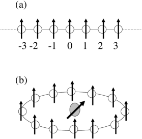
Motivated by these results in the XY modelCarollo ; Zhu2006 , the criticality of geometric phase for other many-body models are investigatedPlastina ; Chen ; Cui ; Yi ; Yuan ; Cozzini . Roughly speaking, there are two patterns (see Fig.1) in literature to investigate the criticality of geometric phase in the many-body systems: (i) Pattern I is order to investigate the relation between geometric phase of the whole many-body system and the system’s quantum phase transition. As illustrate in Fig.1 (a), the geometric phase of the whole N-spin system is calculated and its scaling features in the vicinity of critical points are discussedCarollo ; Zhu2006 ; Hamma ; Plastina ; Chen ; Cui . (b) Pattern II is concerned with the geometric phase of a test qubit as shown in Fig. 1(b). N spins are arranged in a circle and a test qubit in the center possesses homogeneous coupling with all N-spin in the ringQuan ; Yi ; Yuan . The geometric phase of the test qubit may be used to locate the criticality of quantum phase transition exhibiting in the N-spin systemYi ; Yuan . Depending on the couplings between the spins, N-spin chain (ring) in (a) and (b) can be classified as the XY model, the Dicke model and the Lipkin-Meshkoc-Glick model. All these three models exhibit quantum phase transitions, whose features can be captured by the geometric phases in both patterns I and II.

Furthermore, the study of QPTs by using other geometric quantities, such as quantum overlap (quantum fidelity)Zanardi0 , the Riemannian tensorZanardi1 etc., has been put forward and fruitful results have been reported in literature. In particular, GP is a imagine part of quantum geometric tensor and quantum fidelity is a real part, therefore a unified theory of study QPTs from the perspective of quantum geometric tensor has been developedVenuti .

In this paper we will review some aspects of the theoretical understanding that has emerged over the past several years towards understanding the close relation between GPs and QPTs. In section 2, we present the connection between Berry curvature and QPs. Section 3 describes the detailed relation between QPT and GP in the patter I. Section 4 discusses the results in the patter II. Finally, Section 5 presents some discussion and perspective in the topic reviewed in this paper, in particular, we address the recent advances in the connection of some other geometric quantities and QPTs.

II Berry curvature and quantum phase transitions

Let us first address the close relation between quantum phase transitions and geometric phases from an intuitive view. Consider a generic many-body system described by the Hamiltonian $H(\eta)$ with $\eta$ a dimensionless coupling constant. For any reasonable $\eta$, all observable properties of the ground state of $H$ will vary smoothly as $\eta$ is varied. However, there may be special points denoted as $\eta_{c}$, where there is a non-analyticity in some properties of the ground state at zero temperature, $\eta_{c}$ is identified as the position of a quantum phase transition. Non-analytical behavior generally occur at level crossings or avoided level crossingsSachdev . Surprisingly, the geometric phase is able to capture such kinds of level structures and is therefore expected to signal the presence of quantum phase transitions. To address this relation in greater detail, we review geometric phases in a generic many-body system where the Hamiltonian can be changed by varying the parameters ${\bf R}$ on which it depends. The state $|\psi(t)\rangle$ of the system evolves according to Schrodinger equation

$$i\hbar\partial_{t}|\psi(t)\rangle=H({\bf R}(t))|\psi(t)\rangle.$$ (1)

At any instant, the natural basis consists of the eigenstates $|n({\bf R})\rangle$ of $H({\bf R})$ for ${\bf R}={\bf R}(t)$, that satisfy $H({\bf R})|n({\bf R})\rangle=E_{n}({\bf R})|n({\bf R})\rangle$ with energy $E_{n}({\bf R})$ $(n=1,2,3\cdots)$. Berry showed that the GP for a specific eigenstate, such as the ground state ($|g\rangle=|1\rangle$) of a many-body system we concern here, adiabatically undergoing a closed path in parameter space denoted by $C$, is given byBerry

$$\beta_{g}(C)=-\int\int_{C}V_{g}({\bf R})\cdot d{\bf S},$$ (2)

where $d{\bf S}$ denotes area element in ${\bf R}$ space and $V_{g}({\bf R})$ is the Berry curvature given by

$$V_{g}({\bf R})=Im\sum_{n\not=g}\frac{\langle g|\nabla_{\bf R}H|n\rangle\langle n|\nabla_{\bf R}H|g\rangle}{(E_{n}-E_{g})^{2}}.$$ (3)

The energy denominators in Eq.(3) show that the Berry curvature usually diverges at the point of parameter space where energy levels are cross and may have maximum values at avoided level crossings. Thus level crossings or avoided level crossings (seem Fig. 2), the two specific level structures related to quantum phase transitions, are reflected in the geometry of the Hilbert space of the system and can be captured by the Berry curvature of the ground state. However, although the Berry curvature is gauge invariant and is therefore an observable quantity, no feasible experimental setup has been proposed to directly observe it. On the other hand, the area integral of Berry curvature, i.e., the geometric phase may be measured by the interference experiments. Therefore, rather than the Berry curvature, hereafter we will focus on the relation between geometric phase and quantum phase transition, and therefore the proposed relation between them may be experimentally tested.

Figure 2: Schematic representation of the energy level for the many-body systems. The energy levels of the ground state and the excited state cross in (a) and have an avoided crossing in (b). On the one hand, quantum phase transition occurs at level crossings or avoided level crossings, which represents by the parameter $\eta_{c}$; on the other hand, the Berry curvature usually diverges or may have maximum values at the point of parameter $\eta_{c}$.

III Pattern I: QPT and GP of the many-body systems

In this section we review the closed relation between QPTs and GPs for the Pattern I, as shown in Fig.1 (a), where the N-spin chain can be classified as the XY model, the Dicke model and the Lipkin-Meshkoc-Glick model.

III.1 The XY spin chain

Our first example is one-dimensional XY spin chain investigated in detail in Ref.Zhu2006 . The XY model concerns N spin-1/2 particles (qubits) with nearest neighbor interactions and an external magnetic field. The Hamiltonian of the XY spin chain has the following form

$$H=-\sum_{j=-M}^{M}\left(\frac{1+\gamma}{2}\sigma_{j}^{x}\sigma_{j+1}^{x}+\frac{1-\gamma}{2}\sigma_{j}^{y}\sigma_{j+1}^{y}+\lambda\sigma_{j}^{z}\right),$$ (4)

where $\sigma^{\mu}_{j}\ (\mu=x,y,x)$ are the Pauli matrices for the $j$th spin, $\gamma$ represents the anisotropy in the $x-y$ plane and $\lambda$ is the intensity of the magnetic field applied in the $z$ direction. We assume periodic boundary conditions for simplicity and choose $N\ (=2M+1)$ odd to avoid the subtleties connected with the boundary terms. Nevertheless, the differences with other boundary conditions and the even $N$ case are the order to O(1/N) and then negligible in the thermodynamic limit where quantum phase transitions occurLieb ; Osterloh . This XY model encompasses two other well-known spin models: it turns into transverse Ising chain for $\gamma=1$ and the XX (isotropic XY) chain in a transverse field for $\gamma=0$.

In order to derive the geometric phase of ground state in this system, we introduce a new family of Hamiltonians that can be described by applying a rotation of $\phi$ around the $z$ direction to each spin Carollo , i.e.,

$$H_{\phi}=U_{\phi}^{\dagger}HU_{\phi},\ \ U_{\phi}=\prod_{j=-M}^{M}\exp(-i\phi\sigma_{j}^{z}/2).$$ (5)

The critical behavior is independent of $\phi$ as the spectrum $\Lambda_{k}$ (see below) of the system is $\phi$ independent. This class of models can be diagonalized by means of the Jordan-Wigner transformation that maps spins to one-dimensional spinless fermions with creation and annihilation operators $a_{j}$ and $a_{j}^{\dagger}$ via the relations, $a_{j}=(\prod_{l<j}\sigma_{l}^{z})\sigma_{j}^{\dagger}$ Lieb ; Sachdev . Due to the (quasi) translational symmetry of the system we may introduce Fourier transforms of the fermionic operator described by $d_{k}=\frac{1}{\sqrt{N}}\sum_{j}a_{j}\exp(-i2\pi jk/N)$ with $k=-M,\cdots,M$. The Hamiltonian $H_{\phi}$ can be diagonalized by transforming the fermion operators in momentum space and then using the standard Bogoliubov transformation. In this way, we obtain the following diagonalized form of the Hamiltonian,

$$H=\sum_{k}\Lambda_{k}(c_{k}^{\dagger}c_{k}-1),$$ (6)

where the energy of one particle excitation is given by

$$\Lambda_{k}=\sqrt{(\lambda-\cos(2\pi k/N))^{2}+\gamma^{2}\sin^{2}(2\pi k/N)}$$ (7)

and $c_{k}=d_{k}\cos\frac{\theta_{k}}{2}-id_{-k}^{\dagger}e^{2i\phi}\sin\frac{\theta_{k}}{2}$ with the angle $\theta_{k}$ defined by $\cos\theta_{k}=(\cos\frac{2\pi k}{N}-\lambda)/\Lambda_{k}$.

The ground state $|g\rangle$ of $H_{\phi}$ is the vacuum of the fermionic modes described by $c_{k}|g\rangle=0$. Substituting the operator $c_{k}$ into this equation, one obtains the ground state as

$$|g\rangle=\prod_{k=1}^{M}\left(\cos\frac{\theta_{k}}{2}|0\rangle_{k}|0\rangle_{-k}-ie^{2i\phi}\sin\frac{\theta_{k}}{2}|1\rangle_{k}|1\rangle_{-k}\right),$$ (8)

where $|0\rangle_{k}$ and $|1\rangle_{k}$ are the vacuum and single excitation of the $k$th mode, respectively. The ground state is a tensor product of states, each lying in the two-dimensional Hilbert space spanned by $|0\rangle_{k}|0\rangle_{-k}$ and $|1\rangle_{k}|1\rangle_{-k}$. The geometric phase of the ground state, accumulated by varying the angle $\phi$ from $0$ to $\pi$ (Because the Hamiltonian $H_{\phi}$ has bilinear form, $H_{\phi}$ is $\pi$ periodic in $\phi$ ), is described by

$$\beta_{g}=-\frac{i}{M}\int_{0}^{\pi}\langle g|\partial_{\phi}|g\rangle d\phi.$$ (9)

The direct calculation showsCarollo

$$\beta_{g}=\frac{\pi}{M}\sum_{k=1}^{M}(1-\cos\theta_{k}).$$ (10)

The term $\beta_{k}\equiv\pi(1-\cos\theta_{k})$ is a geometric phase for the $k$th mode, and represents the area in the parameter space (which is the Bloch sphere) enclosed by the loop determined by $(\theta_{k},\phi)$. To study the quantum criticality, we are interested in the thermodynamic limit when the spin lattice number $N\ \to\infty$. In this case the summation $\frac{1}{M}\sum_{k=1}^{M}$ can be replaced by the integral $\frac{1}{\pi}\int_{0}^{\pi}d\varphi$ with $\varphi=\frac{2\pi k}{N}$; and then the geometric phase in the thermodynamic limit is given by

$$\beta_{g}=\int_{0}^{\pi}(1-\cos\theta_{\varphi})d\varphi,$$ (11)

where $\cos\theta_{\varphi}=(\cos\varphi-\lambda)/\Lambda_{\varphi}$ with the energy spectrum $\Lambda_{\varphi}=\sqrt{(\lambda-\cos\varphi)^{2}+\gamma^{2}\sin^{2}\varphi}$.

As for quantum criticality in the XY model, there are two regions of criticality, defined by the existence of gapless excitations in the parameter space $(\gamma,\lambda)$: (i) the XX region of criticality described by the segment $(\gamma,\lambda)=(0,(0,1))$; (ii) the critical line $\lambda_{c}=1$ for the whole family of the XY model. For the second critical region, we need to distinguish two universality classes depending on the anisotropy $\gamma$. The critical features are characterized in term of a critical exponent $\nu$ defined by $\xi\sim|\lambda-\lambda_{c}|^{-\nu}$ with $\xi$ representing the correlation length. For any value of $\gamma$, quantum criticality occurs at a critical magnetic field $\lambda_{c}=1$. For the interval $0<\gamma\leq 1$ the models belong to the Ising universality class characterized by the critical exponent $\nu=1$, while for $\gamma=0$ the model belongs to the XX universality class with $\nu=1/2$ Lieb ; Sachdev . The close relation between geometric phase and quantum criticality for the first region has been addressed in Refs.Carollo ; Zhu2006 ; Hamma , here we mainly review the results for the second region, which is clearly more interesting in the sense that the second order quantum phase transitions occur there.

Figure 3: (color online). (a) Geometric phase $\beta_{g}$ of the ground state (b) and its derivative $d\beta_{g}/d\lambda$ as a function of the Hamiltonian parameters $\lambda$ and $\gamma$. The lattice size $N=10001$. There are clear anomalies for the derivative of geometric phase along the critical line $\lambda_{c}=1$.

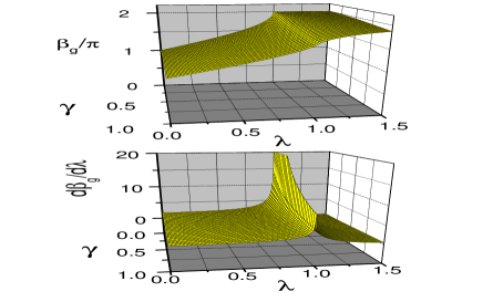
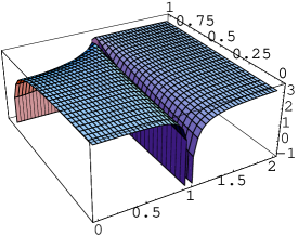
To demonstrate the relation between geometric phase and quantum phase transitions, we plot geometric phase $\beta_{g}$ and its derivative $d\beta_{g}/d\lambda$ with respect to the field strength $\lambda$ and $\gamma$ in Fig.3. A significate feature is notable: the nonanalytical property of the geometric phase along the whole critical line $\lambda_{c}=1$ in the XY spin model is clearly shown by anomalies for the derivative of geometric phase along the same line.

Figure 4: (color online). The derivatives $d\beta_{g}/d\lambda$ for the Ising model ($\gamma=1$) as a function of the Hamiltonian parameter $\lambda$. The curves correspond to different lattice sizes $N=21,101,501,1001,\infty$. With increasing the system sizes, the maximum becomes more pronounced. The inset shows that the position of the maximum changes and tends as $N^{-1.803}$ towards the critical point $\lambda_{c}=1$.

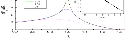
To further understand the relation between geometric phase and quantum criticality, we study the scaling behavior of geometric phases by the finite size scaling approachBarber . We first look at the Ising model. The derivatives $d\beta_{g}/d\lambda$ for $\gamma=1$ and different lattice sizes are plotted in Fig.4. There is no real divergence for finite $N$, but the curves exhibit marked anomalies and the height of which increases with lattice size. The position $\lambda_{m}$ of the peak can be regarded as a pseudo-critical point Barber which changes and tends as $N^{-1.803}$ towards the critical point and clearly approaches $\lambda_{c}$ as $N\to\infty$. In addition, as shown in Ref Zhu2006 , the value of $d\beta_{g}/d\lambda$ at the point $\lambda_{m}$ diverges logarithmically with increasing lattice size as:

$$\frac{d\beta_{g}}{d\lambda}|_{\lambda_{m}}\approx\kappa_{1}\ln N+\mbox{const.},$$ (12)

with $\kappa_{1}=0.3121$. On the other hand, the singular behavior of $d\beta_{g}/d\lambda$ for the infinite Ising chain can be analyzed in the vicinity of the quantum criticality, and we find the asymptotic behavior as

$$\frac{d\beta_{g}}{d\lambda}\approx\kappa_{2}\ln|\lambda-\lambda_{c}|+\mbox{ const.},$$ (13)

with $\kappa_{2}=-0.3123$. According to the scaling ansatz in the case of logarithmic divergence Barber , the ratio $|\kappa_{2}/\kappa_{1}|$ gives the exponent $\nu$ that governs the divergence of the correlation length. Therefore, $\nu\sim 1$ is obtained in our numerical calculation for the Ising chain, in agreement with the well-known solution of the Ising model Lieb .

A cornerstone of QPTs is a universality principle in which the critical behavior depends only on the dimension of the system and the symmetry of the order parameter. The XY model for the interval $\gamma\in(0,1]$ belong to the same universality class with critical exponent $\nu=1$. To verify the universality principle in this model, the scaling behavior for different values of the parameter $\gamma$ has been numerically calculated in Ref. Zhu2006 . The results there shown that the asymptotic behaviors are still described by Eqs. (12) and (13) with $\kappa_{1}$ and $\kappa_{2}$ being $\gamma$-dependent constants, and the same critical exponent $\nu=1$ can be obtained for any $\gamma\in(0,1]$.

Comparing with the $\gamma\not=0$ case, the nature of the divergence of $d\beta_{g}/d\lambda$ at the critical point $(\gamma=0,\lambda=1)$ belongs to a different universality class, and the scaling behavior of geometric phase can be directly extracted from the explicit expression of the geometric phase in the thermodynamic limit. The geometric phase under the thermodynamic limit can be obtained explicitly from Eq.(11) for $\gamma=0$ as

$$\beta_{g}=\left\{\begin{array}[]{ll}2\pi,&(\lambda\leq 1)\\ 2\pi-2\arccos(\lambda),&(\lambda>1)\end{array}\right.$$ (16)

However, it appears from Eq.(10) that the geometric phase $\beta_{g}$ is always trivial for strictly $\gamma=0$ and every finite lattice size $M$, since $\theta_{k}=0$ or $\pi$ for every $k$. The difference between the finite and infinite lattice sizes can be understood from the two limits $N\to\infty$ and $\gamma\to 0$. Assume $\gamma=\epsilon$ with $\epsilon$ an arbitrary small but still finite value, then we can still find a solution $\varphi_{0}$ (it implies $N\to\infty$) for $\cos\varphi_{0}-\lambda=0$ but $\Lambda_{\varphi_{0}}=\epsilon\sqrt{1-\lambda^{2}}\neq 0$ for $\lambda\neq 1$. Then a $\pi$ geometric phase appears for such $\varphi_{0}$ since $\theta_{\varphi_{0}}=\pi/2$. Since $d\beta_{g}/d\lambda=\sqrt{2}(1-\lambda)^{-1/2}$ $(\lambda\to 1^{-})$, we can infer the known result that the critical exponent $\nu=1/2$ for the XX model.

Furthermore, we can confirm the known equivalent $z\nu=1$ between $\nu$ and the dynamical exponent $z$ from the calculations of geometric phases. The dynamical behavior is determined by the expansion of the energy spectrum, i.e., $\Lambda_{\varphi\rightarrow 0}\sim\varphi^{z}[1+(\varphi\xi)^{-z}]$. Then $z=1$ for $\gamma\in(0,1]$ and $z=2$ for $\gamma=0$ are found by the expansion of $\Lambda_{\varphi}$ in the case $\varphi\rightarrow 0$. So we have $z\nu=1$, which is indeed the case for the XY criticalitySachdev .

Therefore, the above results clearly show that all the key ingredients of the quantum criticality are present in the geometric phases of the ground state in the XY spin model.

III.2 The Dicke model

Our second example is the Dicke model Dicke studied in Ref.Plastina ; Chen . It consists of $N$ two-level (qubit) systems coupled to a single Bosonic mode. The Hamiltonian is given by ($\hbar=1$)

$$H=\omega a^{+}a+\Delta J_{x}+\frac{\lambda}{\sqrt{N}}(a^{\dagger}+a)J_{z},$$ (17)

where $a$, $a^{+}$ are the annihilation and creation operators of the Bosonic mode, respectively; $J_{x,z}=\sum_{j=1}^{N}\sigma_{x,z}^{j}$ with $\sigma_{x,z}^{j}$ being the Pauli matrices for the qubit $j$ are collective angular momentum operators for all qubits; $\lambda$ denotes the coupling strength between the atom and field; The parameters $\Delta$ and $\omega$ represent the transition frequency of the atom and Bosonic mode frequency, respectively. The prefactor $1/\sqrt{N}$ is inserted to have a finite free energy per atom in the thermodynamical limit $N\rightarrow\infty$. This Hamiltonian is canonically equivalent to the Dicke Hamiltonian by a $\pi/2$ rotation around the $y$ axis.

As illustrated in Refs.Hepp1 ; Emary , exact solutions may be obtained in the thermodynamic limit by employing a Holstein-Primakoff transformation of the angular momentum algebra. In the thermodynamical limit, the Dicke Hamiltonian undergoes a second quantum phase transition at the critical point $\lambda_{c}=\sqrt{\omega\Delta/2}.$ When $\lambda<\lambda_{c}$, the system is in its normal phase in which the ground state is highly unexcited, while $\lambda>\lambda_{c}$, the system is in its superradiant phase in which both the bosonic field occupation and the spin magnetization acquire macroscopic values.

Similarly to the XY spin model, in order to investigate the geometric phase one changes the original Hamiltonian by the unitary transformation $U_{\phi}=\exp(-i\phi J_{x}/2)$ where $\phi$ is a slowly varying parameter, and then the transformed Hamiltonian is given by

$$H_{\phi}=U^{\dagger}_{\phi}HU_{\phi}=\frac{\omega}{2}[p^{2}+q^{2}+\mathbf{B}\cdot\mathbf{J}],$$ (18)

where the Hamiltonian of the free bosonic field is expressed in terms of canonical variables $q=(a^{\dagger}+a)/\sqrt{2}$ and $p=i(a^{\dagger}-a)/\sqrt{2}$ that obey the standard quantization condition $[q,p]=i$. $\mathbf{B}=(D,\frac{Lq}{\sqrt{N}\sin\phi},\frac{Lq}{\sqrt{N}\cos\phi})$ with dimensionless parameters $D=2\Delta/\omega$ and $L=2\sqrt{2}\lambda/\omega$ is an effective magnetic field felt by the qubits.

In the adiabatic limit, the geometric phase associated with the ground state of the system can be obtained by the Born-Oppenheimer approximation Plastina ; Liberti . In this case, the total wave function of the ground state of the system can be approximated by

$$|\psi_{tot}\rangle=\int dq\varphi(q)|q\rangle\otimes|\chi(q,\phi)\rangle.$$ (19)

Here the state $|\chi(q,\varphi\rangle$ is the state of the adiabatic equation of the qubit (”fast”) part for each fixed value of the slow variable $q$, i.e.,

$$\mathbf{B}\cdot\mathbf{J}|\chi(q,\varphi)\rangle=E(q)|\chi(q,\varphi)\rangle$$ (20)

with $E(q)$ the eigenenergy. It can be proven that the state $|\chi(q,\varphi)\rangle$ can be expressed as a direct product of $N$ qubits as $|\chi(q,\varphi)\rangle=\otimes_{j=1}^{N}|\chi(q,\varphi)\rangle_{j},$ and the state of each qubit can be written as

$$|\chi(q,\varphi)\rangle_{j}=\sin\frac{\alpha}{2}|\uparrow\rangle_{j}-\cos\frac{\alpha}{2}e^{-i\eta}|\downarrow\rangle_{j}$$

with $\cos\alpha=Lq\cos\phi/(\sqrt{N}E(q))$ and $\tan\eta=Lq\sin\phi/(\sqrt{N}D).$ On the other hand, the ground state wave function for the oscillator $\varphi(q)$ is governed by one-dimensional time-independent Schrodinger equation

$$H_{ad}|\varphi(q)\rangle=\frac{\omega}{2}\left(\frac{d^{2}}{dq^{2}}+q^{2}-NE(q)\right)=\varepsilon_{0}|\varphi(q)\rangle,$$

where $\varepsilon_{0}$ is the lowerest eigenvalues of the adiabatic Hamiltonian $H_{ad}$.

Once the total wave function of the ground state is derived, the geometric phase $\beta_{g}$ of the ground state may be derived by the standard method as $\beta_{g}=i\oint\langle\psi_{tot}|d/d\phi|\psi_{tot}\rangle d\varphi$, and the final result is given by

$$\beta_{g}=N\pi\left(1+\frac{\langle J_{x}\rangle}{N}\right).$$ (21)

In the thermodynamic limit, one can show that

$$\frac{\beta_{g}}{N}\left|{}_{N\to\infty}\right.=\left\{\begin{array}[]{ll}\ \ \ \ 0,&(\alpha\leq 1)\\ \pi(1-\frac{1}{\alpha}),&(\alpha>1).\end{array}\right.$$ (22)

Figure 5: The geometric phase $\gamma$ $(\equiv\beta_{g})$ of the ground state and its derivative (inset) for the Dicke model with respect to the parameter $\alpha$ for different values of qubit $N$ and the parameter $D=10$. The geometric phase increases with $\alpha$, and there is a cusplike behavior in the thermodynamic limit at the critical transition point $\alpha=1$.

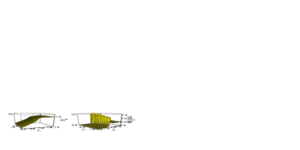
The scaled geometric phase $\beta_{g}/N$ and its derivative with respect to the parameter $\alpha$ for $D=10$ is shown in Fig.5 Plastina . It is evident that the geometric phase increases with increasing the coupling constant at the finite qubit number $N$, while in the thermodynamic limit the geometric phase vanishes when $\alpha<\alpha_{c}$ and has a cusplike behavior at the critical point $\alpha=\alpha_{c}$. In addition, the derivative is discontinuous at the critical point. These results are consistent with the expected behavior of the geometric phase across the critical point, and therefore we add another unusual example to the close relation between geometric phase and quantum phase transition.

III.3 The Lipkin-Meshkov-Glick model

Our third example is the Lipkin-Meshkov-Glick (LMG) model discussed in RefCui . The LMG was first introduced in nuclear physicsLipkin . The LMG model describes a set of N qubits coupled to all others with a strength independent of the position and the nature of the elements and a magnetic field $h$ in the $z$ direction, i.e., the Hamiltonian is given by

$$H=-\frac{1}{N}(S^{2}_{x}+\gamma S^{2}_{y})-hS_{z},$$ (23)

where $\gamma$ is the anisotropy parameter. $S_{\alpha}=\sum_{i=1}^{N}\sigma^{i}_{\alpha}/2(\alpha=x,y,z)$ and the $\sigma_{\alpha}$ is the Pauli operator, N is the total particle number in this system. The prefactor $1/N$ is essential to ensure the convergence of the free energy per spin in the thermodynamic limit. As widely discussed in the literature ( see, e.g., Ref. Botet ), this system displays a second-order quantum phase transition at the critical point $h=1$.

The diagonalization of the LMG Hamiltonian and derivation of the geometric phase can be obtained by a standard procedure, which can be summarized in the following stepsCui : (i) perform a rotation of the spin operators around the $y$ direction, that makes the $z$ axis along the so-called semiclassical magnetization Dusuel in which the Hamiltonian described in Eq.23 has the minimal value in the semiclassical approximation. (ii) Similar to the XY model and the Dicke model, to introduce a geometric phase of the ground state, we consider a system which has a rotation $U(\phi)=e^{-i\phi\tilde{S}_{z}}$ around the new $z$ direction, and then the Hamiltonian becomes $H(\phi)=U^{\dagger}(\phi)HU^{\dagger}(\phi)$. (iii) then we use the Holstein-Primakoff representation,

$$\tilde{S}_{z}(\phi) = N/2-a^{\dagger}a,$$

$$\tilde{S}^{+}(\phi) = (N-a^{\dagger}a)^{1/2}ae^{i\phi},$$

$$\tilde{S}^{-}(\phi) = a^{\dagger}e^{-i\phi}(N-a^{\dagger}a)^{1/2}$$ (24)

in which $a^{\dagger}$ is bosonic operator. Since the $z$ axis is along the semiclassical magnetization, $a^{\dagger}a/N\ll 1$ is a reasonable assumption under low-energy approximation, in which $N$ is large but finite. (iv) the Bogoliubov transformation, which defines the bosonic operator as $b(\phi)=\cosh xae^{i\phi}+\sinh xa^{\dagger}e^{-i\phi}$, where $tanh2x=2\Gamma/\Delta$ with $\Delta=\sin^{2}\theta-\frac{\gamma+\cos^{2}\theta}{2}+h\cos\theta$ and $\Gamma=\frac{\gamma-\cos^{2}\theta}{4}.$ These procedures diagonalize the Hamiltonian to a form

$$H_{diag}(\phi)=Nd+\xi+\Delta^{D}b^{\dagger}(\phi)b(\phi),$$ (25)

where $d=-\frac{1}{4}(\sin^{2}\theta+2h\cos\theta)$, $\xi=\frac{\Delta}{2}(\sqrt{1-\epsilon^{2}}-1)$ $\Delta^{D}=\Delta\sqrt{1-\epsilon^{2}}$, and $\epsilon=\tanh 2x=2\Gamma/\Delta.$ The ground state $|g(\phi)\rangle$ is determined by the relation $b(\phi)|g(\phi)\rangle=0.$ Substituting $b(\phi)$ into the equation above, one finds the ground state,

$$|g(\phi)\rangle = \frac{1}{C}\sum_{n=0}^{[N/2]}\sqrt{\frac{(2n-1)!!}{2n!!}}(-\frac{e^{-i\phi}\sinh x}{e^{i\phi}\cosh x})^{n-1}$$ (26)

$$\cdot(-\sqrt{2}e^{-i\phi}\sinh x)|2n\rangle,$$

where $n!!=n(n-2)(n-4)\cdots$ and $n!!=1$ for $n\leq 0$. $|n\rangle$ is the Fock state of bosonic operator $a^{\dagger}$ and the normalized constant is $C^{2}=\sum_{n=0}^{[N/2]}2\sinh^{2}x\frac{(2n-1)!!}{2n!!}\tanh^{2(n-1)}x$.

The geometric phase $\beta_{g}$ of the ground state accumulated by changing $\phi$ from $0$ to $\pi$ can be derived by the standard method as shown before, and the final result is give byCui

$$\beta_{g}=\pi\left[1-\frac{\sum_{n=0}^{[N/2]}2n\frac{(2n-1)!!}{2n!!}\tanh^{2(n-1)}x}{\sum_{n=0}^{[N/2]}\frac{(2n-1)!!}{2n!!}\tanh^{2(n-1)}x}\right].$$ (27)

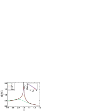
To have some basic ideas about the relation between the geometric phase and phase transition in the LMG model, the geometric phases $\beta_{g}$ as a function of the parameters $(\gamma,h)$ have been plotted in Fig.6Cui . It is notable that the geometric phase $\beta$, independent of the anisotropy, is divergent in the line $h=1$, where the LMG model has been proven to exhibit a second-order phase transitionBotet . The divergence of geometric phase itself, rather then the derivative of geometric phase, shows distinguished character from the XY and Dicke models. This difference stems from that the collective interaction in the LMG model, which is absent in the XY modelCui .

Figure 6: The geometric phase $\beta_{g}$ of the ground state for the LMG model as a function of the parameter $(\gamma,h)$ for $N=200$. The divergence of $\beta_{g}$ is evident at the critical line $h_{c}=1$

The scaling behavior of $\beta_{g}$ has also been studied in Ref Cui . A relatively simply relation $\beta_{g}\approx-N$ is obtained there. Furthermore the scaling is independent of $\gamma$, which means that for different $\gamma$, the phase transitions belong to the same university class. This phenomenon is different from the XY model, in which the isotropic and anisotropic interactions respectively belong to different university classes Zhu2006 .

IV Pattern II: GP of the test qubit and QPT

In this section, we consider a test qubit coupled to a quantum many-body systemYi ; Yuan ; Quan . The Hamiltonian of the whole system may have the form

$$H=H_{t}+H_{S}+H_{I},$$ (28)

where $H_{t}=\mu\mathbf{B}\cdot\mathbf{\sigma}$ stands for the Hamiltonian of the test qubit in a general form, $H_{S}$ represents the Hamiltonian of a many-body system which we are going to study, and $H_{I}$ denotes the coupling between them. We assume that the quantum system described by $H_{S}$ undergoes a quantum phase transition at certain critical points. It is expected that the geometric phase of the test qubit can be used to identify the quantum phase transition of the many-body system. A relatively general formalism to show the close relation between geometric phase of the test qubit and quantum phase transition of the many body system has been developed in Ref.Yi . For solidness, here we address a detailed example studied in Ref.Yuan , where the many-body system with the quantum phase transition is a XY spin chain, i.e.,

$$H_{t}=\mu\sigma^{z}/2+\nu\sigma^{x}/2,$$ (29)

$$H_{S}=-\sum_{l=-M}^{M}\left(\frac{1+\gamma}{2}\sigma_{j}^{x}\sigma_{l+1}^{x}+\frac{1-\gamma}{2}\sigma_{l}^{y}\sigma_{l+1}^{y}+\lambda\sigma_{l}^{z}\right),$$ (30)

$$H_{I}=\frac{\eta}{N}\sum_{l=1}^{N}\sigma^{z}\sigma_{l}^{z}$$ (31)

where the Pauli matrices $\sigma^{x,y,z}$ and $\sigma_{l}^{x,y,z}$ denote the test qubit and the XY spin chain subsystems, respectively. The parameter $\eta$ represents the coupling strength between the test qubit and all spins (qubits) in the spin chain. This model is similar to the Hepp-Coleman modelHepp , which was initially proposed as a model for quantum measurement, and its generalizationNakazato ; Sun .

Following Ref.[15], we assume that the test qubit is initially in a superposition state $|\phi_{t}(0)\rangle=c_{g}|g\rangle+c_{e}|e\rangle$, where $|g\rangle=\left(\sin\frac{\theta_{0}}{2},-\cos\frac{\theta_{0}}{2}\right)^{T}$ and $|e\rangle=\left(\cos\frac{\theta_{0}}{2},\sin\frac{\theta_{0}}{2}\right)^{T}$ with $\theta_{0}=\tan^{-1}(\nu/\mu)$ are ground and excited states of $H_{t}$, respectively. The coefficients $c_{g}$ and $c_{e}$ satisfy the normalization condition, $|c_{g}|^{2}+|c_{e}|^{2}=1$. Then the evolution of the $XY$ spin chain initially prepared in $|\varphi(0)\rangle$, will split into two branches $|\varphi_{\alpha}(t)\rangle=\exp(-iH_{\alpha}t)|\varphi(0)\rangle$ ($\alpha=g,e$), and the total wave function is obtained as $|\psi(t)\rangle=c_{g}|g\rangle\otimes|\varphi_{g}(t)\rangle+c_{e}|e\rangle\otimes|\varphi_{e}(t)\rangle$. Here, the evolutions of the two branch wave functions $|\varphi_{\alpha}(t)\rangle$ are driven, respectively, by the two effective Hamiltonians

$$H_{g}=\langle g|H|g\rangle=H_{S}-\delta\sum_{l=1}^{N}\sigma_{l}^{z}-\Delta,$$ (32)

$$H_{e}=\langle e|H|e\rangle=H_{S}+\delta\sum_{l=1}^{N}\sigma_{l}^{z}+\Delta,$$ (33)

where $\Delta=\sqrt{\mu^{2}+\nu^{2}}/2$ and $\delta=\eta\cos\theta_{0}/N$. Both $H_{g}$ and $H_{e}$ describe the $XY$ model in a transverse field, but with a tiny difference in the field strength. Similar to the method to diagonalize the standard XY spin chain addressed in the patter I, the ground states of the Hamiltonians $H_{\alpha}$ are given by

$$|G_{\alpha}\rangle=\prod_{k=1}^{M}\left(\cos\frac{\theta_{k}^{\alpha}}{2}|0\rangle_{k}|0\rangle_{-k}+i\sin\frac{\theta_{k}^{\alpha}}{2}|1\rangle_{k}|1\rangle_{-k}\right),$$ (34)

where $\cos\theta_{k}^{\alpha}=\epsilon_{k}^{\alpha}/\Lambda_{k}^{\alpha}$ with $\Lambda_{k}^{\alpha}=\sqrt{\epsilon_{k,\alpha}^{2}+\gamma^{2}\sin^{2}\frac{2\pi k}{N}}$ and $\epsilon_{k,\alpha}=\lambda-\cos\frac{2\pi k}{N}+\kappa_{\alpha}\delta$ ($\kappa_{g}=-\kappa_{e}=1$). $|0\rangle_{k}$ and $|1\rangle_{k}$ are the vacuum and single excitation of the $k$th mode, respectively. Here $d_{k}$ is similarly defined as the standard XY model (see section 3.1).

Now we turn to study the behaviors of the geometric phase for the test qubit when the XY spin chain is at its ground state. Due to the coupling, it is expected that the geometric phase for the test qubit will be profoundly influenced by the occurrence of quantum phase transition in spin-chain environment. Since we are interesting to the quantum phase transition, which is the property of the ground state, we assume that the $XY$ spin chain is adiabatically in the ground state $|G_{g}(\{\theta_{k}^{g}\})\rangle$ of $H_{g}$. In this case the effective mean-field Hamiltonian for the test qubit is given by

$$H_{eff} = H_{t}+\langle G_{g}|H_{I}|G_{g}\rangle$$ (35)

$$= \left(\frac{\mu}{2}+\frac{2\eta}{N}\sum_{k=1}^{M}\cos\theta_{k}^{(g)}\right)\sigma^{z}+\frac{\nu}{2}\sigma^{x}.$$ (36)

In order to generate a geometric phase for the test qubit, as usual, we change the Hamiltonian by means of a unitary transformation: $U(\phi)=\exp\left(-i\frac{\phi}{2}\sigma_{z}\right),$ where $\phi$ is a slowly varying parameter, changing from $0$ to $\pi$. The transformed Hamiltonian can be written as $H(\phi)=U^{+}(\phi)H_{eff}U(\phi)$, i.e.,

$$H(\phi)=\left(\frac{\mu}{2}+\frac{2\eta}{N}\sum_{k=1}^{M}\cos\theta_{k}^{(g)}\right)\sigma^{z}+\frac{\nu}{2}(\sigma^{x}\cos\phi-\sigma^{y}\sin\phi).$$ (37)

Then the eigen-energies of the effective Hamiltonian for the test qubit are given by

$$E_{e,g}=\pm\sqrt{\left(\frac{\mu}{2}+\frac{2\eta}{N}\sum_{k=1}^{M}\cos\theta_{k}^{(g)}\right)^{2}+\frac{\nu^{2}}{4}}.$$ (38)

and the corresponding eigenstates are given by

$$|g\rangle=\left(\begin{array}[]{l}\sin\frac{\theta}{2}\\ -\cos\frac{\theta}{2}e^{-i\phi}\end{array}\right),|e\rangle=\left(\begin{array}[]{l}\cos\frac{\theta}{2}\\ \sin\frac{\theta}{2}e^{-i\phi}\end{array}\right),$$ (39)

where $\sin\theta=\nu/2E_{e}$.

The accumulated ground-state geometric phase $\beta_{g}$ for the test qubit by varying $\phi$ from zero to $\pi$ can be derived from the standard integral $\int_{0}^{\pi}\langle G_{g}|\partial_{\phi}|G_{g}\rangle d\phi,$ and it is easy to find that

$$\beta_{g}=\pi\left(1+\frac{\mu+4\eta f(\lambda,\gamma,N)}{\sqrt{[\mu+4\eta f(\lambda,N)]^{2}+\nu^{2}}}\right),$$ (40)

where $f(\lambda,\gamma,N)=\frac{1}{N}\sum_{k=1}^{M}\cos\theta_{k}^{(g)}$. In the thermodynamic limit $N\rightarrow\infty$, the summation in $f(\lambda,\gamma,N)$ can be replaced by the integral as follows:

$$f(\lambda,\gamma,N)|_{N\rightarrow\infty}=\frac{1}{2\pi}\int_{0}^{\pi}\frac{\lambda-\cos\varphi}{\sqrt{(\lambda-\cos\varphi)^{2}+\gamma^{2}\sin^{2}\varphi}}d\varphi.$$ (41)

The geometric phase $\beta_{g}$ and its derivative $d\beta_{g}/d\lambda$ with respect to the parameter $(\lambda,\gamma)$ of the XY model are plotted in Fig.7. As expected, the nonanalytic behavior of the geometric phase and the corresponding anomalies in its derivative $d\beta_{g}/d\lambda$ along the critical lines $\lambda_{c}=1$ are clear. All these features are very similar to those in the XY spin chain in patter I (see section 3.1).

Figure 7: (a) Ground-state geometric phase $\beta_{g}$ of the test qubit and (b) its derivative $d\beta_{g}/d\lambda$ as a function of the spin-chain parameter $(\lambda,\gamma)$. The anomalies for the derivative of geometric phase is clear along the critical line $\lambda_{c}=1$. The other parameters: $\mu=0.1$, $\nu=2$, and $\eta=0.5$.

Figure 8: The derivatives $d\beta_{g}/d\lambda$ for the test qubit which is coupling to the Ising spin chain ($\gamma=1$), with respect to the parameter $\lambda$ for different lattice sizes $N=12,51,251,501,\infty$. With increasing the system sizes, the maximum becomes more pronounced and the position of the maximum clearly approaches $\lambda_{c}=1$ as $N\rightarrow\infty$. The inset shows the size scaling of the position of the peak occurred in $d\beta_{g}/d\lambda$ (circles) and the function $f(\lambda,\gamma,N)$ (squares).

To further understand the relation between GPs and QPTs in this system, let us consider the case of $XX$ spin model ($\gamma=0$) in which geometric phase can be analytically derived. In the thermodynamic limit, the function $f(\lambda,\gamma,N)$ in Eq.41 can be derived explicitly for $\gamma=0$ as $f=1/2-\arccos(\lambda)/\pi$ when $\lambda\leq 1$ and $f=1/2$ when $\lambda>1$. In this case, the geometric phase of the test qubit is given by

$$\beta_{g}\bigr{|}_{N\rightarrow\infty}=\left\{\begin{array}[c]{l}\pi\left(1+\frac{\mu+2g[1-2\arccos(\lambda)/\pi]}{\sqrt{\left(\mu+2g[1-2\arccos(\lambda)/\pi]\right)^{2}+\nu^{2}}}\right)\ \ \ \ \ (\lambda\leq 1)\\ \pi\left(1+\frac{\mu+2g}{\sqrt{\left(\mu+2g\right)^{2}+\nu^{2}}}\right)\ \ \ \ \ \ \ \ \ \ \ \ \ \ \ \ \ \ \ \ \ \ (\lambda>1)\end{array}\right.$$ (42)

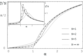
which clearly shows a discontinuity at $\lambda=\lambda_{c}=1$. The derivative $d\beta_{g}/d\lambda$ as a function of $\lambda$ for $\gamma=1$ and different lattice sizes are plotted in Fig. 8 Yuan . It is notable that the derivative of geometric phase is peaked around the critical point $\lambda_{c}=1$. The amplitude of the peak is prominently enhanced by increasing the lattice size of the spin chain. The size dependent of the peak position $\lambda_{m}$ for $d\beta_{g}/d\lambda$ is shown in the inset of Fig. 8. For comparison, the size dependence of the peak position in $\lambda$ space for the derivative $df/d\lambda$ are also shown in the inset (squires). The scaling behavior of $d\beta_{g}/d\lambda$ and $df/d\lambda$ are evident in the figure. All these features are similar to these exhibit in the XY spin chain of the patter I. Therefore, we can see that QPTs of the XY spin chain are faithfully reflected by the behaviors of the ground-state GP and its derivative of the coupled test qubit.

V Summary and concluding remarks

Quantum phase transition plays a key role in condensed matter physics, while the concept of geometric phase is fundamental in quantum mechanics. However, no relevant relation was recognized before recent work. In this paper, we present a review of the connection recently established between these two interesting fields. Phases and phase transitions are traditionally described by the Ginzburg-Landau symmetry-breaking theory based on order parameters and long rang correlation. Recent develops offer other perspectives to understand quantum phase transitions, such as topological order, quantum entanglement, geometric phases and other geometric quantities. Before conclusion, we would like to briefly address that, rather than geometric phase reviewed in this paper, the deep relationship between some other geometric quantities and quantum phase transitions has also been revealed.

Quantum fidelity. Recently an approach to quantum phase transitions based on the concept of quantum fidelity has been put forwardZanardi0 ; Zhou . In this approach, quantum phase transitions are characterized by investigating the properties of the overlap between two ground states corresponding to two slightly different set of parameters. The overlap between two states can be considered as a Hilbert-space distance, and is also called quantum fidelity from the perspective of quantum information. A drop of the fidelity with scaling behavior is observed in the vicinity of quantum phase transition and then quantitative information about critical exponents can be extractedCozzini ; Cozzini1 . The physical intuition behind this relation is straightforward. Quantum phase transitions mark the separation between regions of the parameter space which correspond to ground state having deeply different structural properties. Since the fidelity is a measure of the state-state distance, the dramatic change of the structure of the ground state around the quantum critical point should result in a large distance between two ground states. The study of QPTs based on quantum fidelity (overlap) has been reported for several statistical modelsZanardi0 ; Zhou ; Zanardi_JSM ; Gu1 ; Yi_Hann . In addition, the dynamic analogy of quantum overlap is the Loschmidt echo; it has been shown that the Loschmidt echo also exhibits scaling behavior in the vicinity of the critical pointQuan ; Quan2 ; Ou .

The Riemannian tensor. It has been shown that the fidelity approach can be better understood in terms of a Riemannian metric tensor $g$ defined over the parameter manifoldZanardi1 . In this approach, the manifold of coupling constants parameterizing the system’s Hamiltonian can be equipped with a (pseudo) Riemannian tensor $g$ whose singularities correspond to the critical regions.

We have presented that one can study quantum phase transitions from the perspective of some geometric objects, such as geometric phase, quantum fidelity and the Riemannian tensor. Surprisingly, All these approaches share the same origin and can be therefore unified by the concept of quantum geometric tensors. We now briefly recall the formal setting developed in Ref.Venuti . For each element $\eta$ of the parameter manifold $\mathcal{M}$ there is an associated Hamiltonian $H(\eta)=\sum_{n=0}^{dim\mathcal{H}}E_{n}(\eta)|\Psi_{n}(\eta)\rangle\langle\Psi_{n}(\eta)|$ $(E_{n+1}>E_{n})$, acting over a finite-dimensional state space $\mathcal{H}$. If $|\Psi(\eta)\rangle$ represents the unique ground state of $H(\eta)$, then one has the mapping $\Psi_{0}:\mathcal{M}\rightarrow\mathcal{H}:\eta\rightarrow|\Psi(\eta)\rangle$. In this case, one can define a quantum geometric tensor which is a complex hermitean tensor in the parameter manifold $\mathcal{M}$ given by Provost

$$Q_{\mu\nu}\equiv\langle\partial_{\mu}\Psi_{0}|\partial_{\nu}\Psi_{0}\rangle-\langle\partial_{\mu}\Psi_{0}|\Psi_{0}\rangle\langle\Psi_{0}|\partial_{\nu}\Psi_{0}\rangle,$$ (43)

where the indices $\mu$ and $\nu$ denote the coordinates of $\mathcal{M}$. The real part of the quantum geometric tensor $Q$ is the Riemannian metric, while the imaginary part is the curvature form giving rise to a geometric phaseVenuti . Similar to the heuristic argument that we have addressed for the singularity of Berry curvature in the vicinity of quantum phase transition, it has been shown that the quantum geometric tensor also obeys critical scaling behaviorVenuti ; Zanardi0 ; Zhu2006 . Therefore, viewing quantum phase transitions from the perspectives of geometric phase and quantum fidelity can be unified by the concept of quantum geometric tensor.

In conclusion, we presented a review of criticality of geometric phase established recently, in which geometric phase associated with the many-body ground state exhibits universality, or scaling behavior in the vicinity of the critical point. In addition, we addressed that one can investigate quantum phase transition from the views of some typical geometric quantities. The closed relation recently recognized between quantum phase transitions and quantum geometric tensor may open attractive avenues and fruitful dialog between different scientific communities..

References

- (1) S. Sachdev, Quantum Phase Transitions (Cambridge Univ. Press, Cambridge, U. K., 1999).
- (2) X. G. Wen, Quantum field theory of many-body systems (Oxford University Press, Oxford, 2004).
- (3) T. J. Osborne and M. A. Nielsen, Phys. Rev. A 66, 032110 (2002); A. Osterloh et al., Nature (London), 416, 608 (2002); G. Vidal et al., Phys. Rev. Lett.90, 227902 (2003).
- (4) Y. Chen, P. Zanardi, Z. D. Wang, and F. C. Zhang, New J. Phys. 8, 97 (2006); S. J. Gu, S. S. Deng, Y. Q. Li, and H. Q. Lin, Phys. Rev. Lett. 93, 086402 (2004).
- (5) A. C. M. Carollo and J. K. Pachos, Phys. Rev. Lett. 95, 157203 (2005).
- (6) S. L. Zhu, Phys. Rev. Lett. 96, 077206 (2006).
- (7) P. Zanardi and N. Paunkovic, Phys. Rev. E 74, 031123 (2006).
- (8) P. Zanardi, P. Giorda, and M. Cozzini, quant-ph/0701061 (2007).
- (9) H. Q. Zhou and J. P. Barjaktarevic, arXiv:cond-mat/0701608 (2007); H. Q. Zhou, J. H. Zhao, and B. Li, arXiv:0704.2940 (2007).
- (10) L. C. Venuti and P. Zanardi, arXiv: 0705.2211 (2007).
- (11) H. T. Quan, Z. Song, X. F. Liu, P. Zanardi, and C. P. Sun, Phys. Rev. Lett. 96, 140604 (2006).
- (12) Y. Aharonov and D. Bohm, Phys. Rev. 115, 485 (1959).
- (13) C. N. Yang, Phys. Rev. Lett. 33, 445 (1974).
- (14) T. T. Wu and C. N. Yang, Phys. Rev. D 12 3845 (1975).
- (15) M. V. Berry, Proc. R. Soc. London A 392, 45 (1984).
- (16) B. Simon, Phys. Rev. Lett. 51 2167 (1983).
- (17) Y. Aharonov and J. Anandan, Phys. Rev. Lett. 58, 1593 (1987); Y. S. Wu and H. Z. Li, Phys. Rev. B 38, 11907 (1988).
- (18) J. Samuel and R. Bhandari, Phys. Rev. Lett. 60, 2339 (1988).
- (19) E. Sjoqvist et al., Phys. Rev. Lett. 85, 2845 (2000); D. M. Tong et al., ibid. 93, 080405 (2004); J. Du et al., ibid. 91, 100403 (2003); X.X.Yi, L. C. Wang, and T. Y. Zheng, ibid. 92, 150406 (2004); M. Ericsson et al., ibid. 94, 050401 (2005).
- (20) S. L. Zhu, Z. D. Wang, and Y. D. Zhang, Phys. Rev. B, 61, 1142 (2000).
- (21) Geometric Phases in Physics, edited by A. Shapere and F. Wilczek (World Scientific, Singapore, 1989).
- (22) H. Z. Li, Global Properties of Simple Physical Systems - Berry’s Phase and others (Shanghai Scientific and Technical Publishers, Shanghai, 1998).
- (23) A. Bohm et al., The Geometric Phase in Quantum Systems (Springer, New York, 2003).
- (24) D. J. Thouless, P. Ao, and Q. Niu, Phys. Rev. Lett. 76, 3758 (1996); D. Arovas, J. R. Schrieffer, and F. Wilczek, ibid., 53, 722 (1984); R. Resta, Rev. Mod. Phys. 66, 899 (1994).
- (25) A. F. Morpurgo et al., Phys. Rev. Lett. 80, 1050 (1998); S. L. Zhu and Z. D. Wang, ibid., 85, 1076 (2000).
- (26) P. Zanardi and M. Rasetti, Phys. Lett. A 264, 94 (1999); J. Pachos, P. Zanardi and M. Rasetti, Phys. Rev. A 61, 010305(R) (1999); J. A. Jones et al., Nature 403, 869 (2000); L. M. Duan, J. I. Cirac, and P. Zoller, Science 292, 1695 (2001); S. L. Zhu and Z. D. Wang, Phys. Rev. Lett. 89, 097902 (2002); ibid.,91 187902 (2003).
- (27) E. Lieb, T. Schultz, and D. Mattis, Ann. Phys. 16, 407 (1961); E. Barouch and B. McCoy, Phys. Rev. A 3, 786 (1971); P. Pfeuty, Ann. Phys. 57, 79 (1970).
- (28) A. Hamma, quant-ph/0602091 (2006).
- (29) M. N. Barber in Phase Transition and Critical Phenomena, Edited by C. Domb and J. L. Lebowitz, Vol. 8, P145 ( Academic Press, London, 1983).
- (30) F. Plastina, G. Liberti, and A. Carollo, Europhys. Lett. 76, 182 (2006).
- (31) G. Chen, J. Li, and J. Q. Liang, Phys. Rev. A 74, 054101 (2006).
- (32) H. T. Cui, K. Li, and X. X. Yi, Phys. Lett. A 360, 243 (2006).
- (33) X. X. Yi amd W. Wang, Phys. Rev. A 75, 032103 (2007).
- (34) Z. G. Yuan, P. Zhang, and S. S. Li, Phys. Rev. A 75, 012102 (2007).
- (35) M. Cozzini, P. Giorda, and P. Zanardi, Phys. Rev. B 75, 014439 (2007).
- (36) R. H. Dicke, Phys. Rev. 93, 99 (1954).
- (37) K. Hepp and E. Lieb, Ann. Phys. 76, 360 (1973); Phys. Rev. A 8, 2517 (1973).
- (38) C. Emary and T. Brands, Phys. Rev. Lett. 90, 044101 (2003).
- (39) G. Liberti, R. L. Zaffino, F. Piperno, and F. Plastina, Phys. Rev. A 73, 032346 (2006).
- (40) H. J. Lipkin, N. Meshkov, and A. J. Glick, Nucl. Phys. 62, 188 (1965).
- (41) R. Botet, R. Jullien, P. Pfeuty, Phys. Rev. Lett. 49, 478 (1982); R. Botet, R. Jullien, Phys. Rev. B 28, 3955 (1982).
- (42) D. Dusuel and J. Vidal, Phys. Rev. Lett. 93, 237204 (2004).
- (43) K. Hepp, Helv. Phys. Acta 45, 237 (1972); J. S. Bell, Helv. Phys. Acta 48, 93 (1975).
- (44) H. Nakazato and S. Pascazio, Phys. Rev. Lett. 70, 1 (1993).
- (45) C. P. Sun, Phys. Rev. A 48, 898 (1993).
- (46) M. Cozzini, R. Ionicioiu, and P. Zanardi, cond-mat/0611727.
- (47) P. Zanardi, M.Cozzini, and P. Giorda, J. Stat. Mech.: Theory Exp. 2007, L02002.
- (48) W.L.You,Y.W.Li and S.J. Gu, arXiv.org:quant-ph/0701077(2007).
- (49) X.X.Yi,H. Wang, and W.Wang, cond-mat/0601318 (2006).
- (50) Y. C. Ou and H. Fan, J. Phys. A: Math. Theor. 40, 2455 (2007).
- (51) H. T. Quan, Z. D. Wang, C. P. Sun, arXiv:quant-ph/0702268 (2007).
- (52) J. P. Provost and G. Vallee, Commun. Math. Phys. 76, 289 (1980).