Meissner effect without superconductivity from a chiral d-density wave

Abstract

We demonstrate that the formation of a chiral d-density wave (CDDW) state generates a Topological Meissner effect (TME) in the absence of any kind of superconductivity. The TME is identical to the usual superconducting Meissner effect but it appears only for magnetic fields perpendicular to the plane while it is absent for in plane fields. The observed enhanced diamagnetic signals in the non-superconducting pseudogap regime of the cuprates may find an alternative interpretation in terms of a TME, originating from a chiral d-density wave pseudogap.

The Meissner effect is considered to be the most direct signature of superconductivity Schrieffer . However, the surprising observations of such enhanced diamagnetic signals Exp Nerst Magnet well above the superconducting transition temperature in the pseudogap regime of the cuprates pseudogap review , constitute a fascinating puzzle. There are two proposals for the nature of this regime that appear to dominate. The first, associates the pseudogap with a $d_{x^{2}-y^{2}}$ density wave (DDW) Chakravarty ; Affleck , also called orbital antiferromagnet DDW ; Nersesyan , which normally competes with superconductivity. The second associates the pseudogap with spontaneous vortex-antivortex unbinding leading to incoherent superconductivity Emery that should persist well above the superconducting $T_{c}$. This theory is reminiscent of the well known Kosterlitz-Thouless transition KT .

The available ARPES ARPES and STM STM experiments cannot differentiate a SC from a density wave (DW) gap, and therefore appear somehow incapable in settling directly the issue. On the other hand, the unusual Nernst effect and most importantly, the enhanced diamagnetic signal that accompanies it for a very large temperature region above the SC critical temperature Exp Nerst Magnet , has been considered as a major argument in favor of the incoherent SC scenario. In fact, the enhanced diamagnetism is viewed as a signature of the usual Meissner effect associated solely with the SC state, and would therefore contradict the $d_{x^{2}-y^{2}}$ density wave scenario since no Meissner effect was expected in that case Nersesyan .

In this letter we put forward the Topological Meissner effect (TME), that results from a chiral $d_{xy}+id_{x^{2}-y^{2}}$ density wave (CDDW) state. In fact, the Nernst region of the pseudogap regime may well be associated with a CDDW. The most intriguing property of a CDDW is that parity (${\cal P}$) and time-reversal (${\cal T}$) violation induces Chern-Simons terms in the effective action of the electromagnetic field, providing the possibility of the TME and the Spontaneous Quantum Hall effect (SQHE) earlier discussed KVL ; Yakovenko ; Kerler ; Goryo ; Furusaki ; Horovitz ; Volovik . As we shall demonstrate, the TME is described by the same equation we find in the usual Meissner effect of a superconductor. Though, its origin is radically different. In our system we encounter the realization of Parity Anomaly Yakovenko ; parityanomaly , with the emerging Chern-Simons terms providing a topological mass to the electromagnetic field, in a gauge invariant manner Deser ; Fradkin . Moreover, the possession of chirality perpendicular to the plane, implies that the TME is strongly anisotropic. Particularly, it takes place for magnetic fields perpendicular to the plane while it is absent for in plane fields, in accordance with the experimental observations Exp Nerst Magnet . Note finally that a chiral d-density wave state has also been shown recently Tewari to explain the experimental results concerning the Polar Kerr effect in YBCO Xia .

In order to demonstrate how the TME arises, we shall consider the following BCS hamiltonian for the CDDW

$${\cal H}_{{\small CDDW}}^{\phantom{{\dagger}}}=\frac{1}{2}\sum_{\bm{k}}\left(\Delta_{\bm{k}}^{\phantom{{\dagger}}}c_{\bm{k}}^{{\dagger}}c_{\bm{k+Q}}^{\phantom{{\dagger}}}+\Delta^{*}_{\bm{k}}c_{\bm{k+Q}}^{{\dagger}}c_{\bm{k}}^{\phantom{{\dagger}}}\right),$$ (1)

which describes a $d_{xy}+id_{x^{2}-y^{2}}$ state characterized by the wave-vector $\bm{Q}=(\pi,\pi)$, which is commensurate to the lattice ($\bm{k}+2\bm{Q}=\bm{k}$). Since spin degrees of freedom do not get involved we have considered spinless electrons, so that all our results will refer to one spin component. Furthermore, we use $g_{\mu\nu}^{\phantom{{\dagger}}}=(1,-1,-1)$, $k^{i}=\bm{k}=(k_{x}^{\phantom{{\dagger}}},k_{y}^{\phantom{{\dagger}}})$, $k^{\mu}=k=(\omega,\bm{k}$), $q^{\mu}=q=(q_{0}^{\phantom{{\dagger}}},\bm{q})$, $\mu=0,1,2$, $i=1,2$, $e>0$, $\hbar=1$ and we assume that repeated indices are summed. In the derivation of the Chern-Simons terms we shall restrict ourselves to the zero temperature case while necessary extensions to finite temperatures will be afterwards performed. In addition, the summation in $\bm{k}-$space is all over the whole $1^{st}$ Brillouin zone rather than the reduced Brillouin zone. This implies that the operators $c_{\bm{k}}^{\phantom{{\dagger}}}$ and $c_{\bm{k+Q}}^{\phantom{{\dagger}}}$ do not describe independent degrees of freedom.

In Eq.(1) we have introduced the CDDW order parameter $\Delta_{\bm{k}}^{\phantom{{\dagger}}}=\eta\Delta\sin k_{x}^{\phantom{{\dagger}}}\sin k_{y}^{\phantom{{\dagger}}}+i\Delta\left(\cos k_{x}^{\phantom{{\dagger}}}-\cos k_{y}^{\phantom{{\dagger}}}\right)$, where $\Delta$ is the modulus of the $id_{x^{2}-y^{2}}$ order parameter, $\eta$ defines the relative magnitude of the two components and also determines the direction of the chirality of the state. The chiral character of the state implies the existence of an intrinsic angular momentum in $\bm{k}-$space, perpendicular to the plane, originating from ${\cal P-T}$ violation. Specifically, the $d_{x^{2}-y^{2}}$ component violates ${\cal T}$ as it is imaginary, while the $d_{xy}$ component is odd under ${\cal P}$ in two dimensions, which is defined as $(k_{x},k_{y})\rightarrow(k_{x},-k_{y})$.

In order to obtain the total electronic Hamiltonian ${\cal H}$, we have to add the corresponding kinetic part ${\cal H}_{kin}^{\phantom{{\dagger}}}$. For the kinetic part we keep only the nearest neighbors hopping term $\epsilon_{\bm{k}}^{\phantom{{\dagger}}}=-t\left(\cos k_{x}^{\phantom{{\dagger}}}+\cos k_{y}^{\phantom{{\dagger}}}\right)$ satisfying the nesting condition $\epsilon_{\bm{k+Q}}^{\phantom{{\dagger}}}=-\epsilon_{\bm{k}}^{\phantom{{\dagger}}}$, while we also set the chemical potential equal to zero. Our approximation can be justified by considering that our system is close to half-filling. Under these conditions the excitation spectrum consists of two bands which are fully gapped leading to the topological quantization of the Hall conductance KVL ; Yakovenko ; Kerler ; Goryo ; Furusaki ; Horovitz ; Volovik , which is the coefficient of the Chern-Simons terms. Omitting the next nearest neighbors hopping term $\delta_{\bm{k}}^{\phantom{{\dagger}}}=t^{\prime}\cos k_{x}\cos k_{y}$ does not alter qualitatively the occurrence of the TME. However, its inclusion would destroy the quantization of the Hall conductance, as in this case, the system is not fully gapped. Similar effects would arise in the presence of disorder or by including the $z$-axis hopping term.

Under this conditions, the total Hamiltonian of the system becomes ${\cal H}=\frac{1}{2}\sum_{\bm{k}}\left[\epsilon_{\bm{k}}^{\phantom{{\dagger}}}\left(c_{\bm{k}}^{{\dagger}}c_{\bm{k}}^{\phantom{{\dagger}}}-c_{\bm{k+Q}}^{{\dagger}}c_{\bm{k+Q}}^{\phantom{{\dagger}}}\right)+\right.$ $\left.\left(\Delta_{\bm{k}}^{\phantom{{\dagger}}}c_{\bm{k}}^{{\dagger}}c_{\bm{k+Q}}^{\phantom{{\dagger}}}+h.c.\right)\right]$. We obtain a compact representation of ${\cal H}$ by introducing the spinor $\Psi^{{\dagger}}_{\bm{k}}=\frac{\phantom{.}1}{\sqrt{2}}(c^{{\dagger}}_{\bm{k}}\phantom{.}c^{{\dagger}}_{\bm{k+Q}})$, the isospin Pauli matrices $\bm{\tau}$ and the vector $\bm{g}_{\bm{k}}^{\phantom{{\dagger}}}\equiv({\cal R}e\Delta_{\bm{k}}^{\phantom{{\dagger}}},-{\cal I}m\Delta_{\bm{k}}^{\phantom{{\dagger}}},\epsilon_{\bm{k}}^{\phantom{{\dagger}}})$. This yields ${\cal H}=\sum_{\bm{k}}\Psi^{{\dagger}}_{\bm{k}}\phantom{.}\bm{g}_{\bm{k}}^{\phantom{{\dagger}}}\cdot\bm{\tau}\phantom{.}\Psi_{\bm{k}}^{\phantom{{\dagger}}}$. The latter indicates that the ground state of the system depends on the orientation of the $\bm{g}$ vector in isospin space. As a result, this hamiltonian supports skyrmion solutions which imply the presence of a Chern-Simons action (see e.g. Volovik ).

To reveal the emerging Chern-Simons terms, we have to take into account the fluctuations of the $U(1)$ gauge field $A^{\mu}$. We add to the Hamiltonian the term ${\cal H}_{em}^{\phantom{{\dagger}}}=\int\frac{\rm{d}^{2}q}{(2\pi)^{2}}\sum_{\bm{k}}\Psi_{\bm{k+q}}^{{\dagger}}\Gamma^{\mu}_{\bm{k+q,k}}A_{\mu}^{\phantom{{\dagger}}}(\bm{q})\Psi_{\bm{k}}^{\phantom{{\dagger}}}-\int\frac{\rm{d}^{2}q}{(2\pi)^{2}}\sum_{\bm{k}}\Psi_{\bm{k+q}}^{{\dagger}}\frac{e^{2}}{2m}A^{i}(-\bm{q})A_{i}^{\phantom{{\dagger}}}(\bm{q})\Psi_{\bm{k}}^{\phantom{{\dagger}}}$, which describes the interaction of the gauge field with the electrons. We have introduced the paramagnetic interaction vertex $\Gamma^{\mu}_{\bm{k+q},\bm{k}}=-(e\phantom{.},\phantom{.}e\frac{\partial\phantom{{\dagger}}}{\partial k^{i}}\phantom{.}\bm{g}_{\bm{k}}^{\phantom{{\dagger}}}\cdot\bm{\tau})$, where $\mu=0,1,2$ and $i=1,2$. At one-loop level, the effective action $S_{em}^{\phantom{{\dagger}}}$ is given by the relation $S_{em}^{\phantom{{\dagger}}}=\frac{1}{2}\int\frac{{\rm d}^{3}q}{(2\pi)^{3}}\phantom{.}A^{\mu}(-q)\Pi_{\mu\nu}(q)A^{\nu}(q)$, with the Polarization tensor $\Pi_{\mu\nu}$, defined as $\Pi^{\mu\nu}(q)=\frac{i}{2}\int_{k}Tr\left({\cal G}_{k}^{\phantom{{\dagger}}}\Gamma^{\mu}_{k,k+q}{\cal G}_{k+q}^{\phantom{{\dagger}}}\Gamma^{\nu}_{k+q,k}\right)-\frac{\phantom{.}e^{2}}{m}\rho_{e}^{\phantom{{\dagger}}}\delta_{i,j}^{\phantom{{\dagger}}}$. $\rho_{e}^{\phantom{{\dagger}}}$ is the two-dimensional electronic density (without including spin), $Tr$ denotes trace over isospin indices, ${\cal G}_{k}^{\phantom{{\dagger}}}$ is the CDDW fermionic propagator and we have used the abbreviation $\int_{k}=\int\frac{{\rm d}\omega}{2\pi}\sum_{\bm{k}}$. Computing $\Pi_{\mu\nu}$ up to linear order in $q$, yields the Chern-Simons action

$$S_{CS}^{\phantom{{\dagger}}}=\int{\rm d^{3}}x\phantom{.}\frac{\sigma_{xy}}{4}\varepsilon_{\mu\nu\lambda}^{\phantom{{\dagger}}}A^{\mu}F^{\nu\lambda},$$ (2)

with $F_{\mu\nu}=\partial_{\mu}A_{\nu}-\partial_{\nu}A_{\mu}$. The coefficient of the Chern-Simons action is the Hall conductance $\sigma_{xy}$. It can be shown that it is a topological invariant, reflecting the existence of a topologically non trivial, ${\cal P-T}$ violating ground state (see e.g. Volovik ). Using Eq.(2) we obtain

$$\sigma_{{{xy}}}^{\phantom{{\dagger}}}=\frac{i}{2!}\varepsilon_{0ji}\frac{\partial\Pi_{0i}^{\phantom{{\dagger}}}}{\partial q^{j}}=\frac{e^{2}}{4\pi}\widehat{N}=\frac{e^{2}}{2\pi},$$ (3)

where we have introduced the winding number of the unit vector $\hat{\bm{g}}_{\bm{k}}^{\phantom{{\dagger}}}={\bm{g}}_{\bm{k}}^{\phantom{{\dagger}}}/{\mid\bm{g}_{\bm{k}}^{\phantom{{\dagger}}}\mid}$,

$$\widehat{N}=\frac{1}{4\pi}\int{\rm d}^{2}k\phantom{{\dagger}}\hat{\bm{g}}_{\bm{k}}^{\phantom{{\dagger}}}\cdot\left(\frac{\partial\hat{\bm{g}}_{\bm{k}}^{\phantom{{\dagger}}}}{\partial k_{{x}}}\times\frac{\partial\hat{\bm{g}}_{\bm{k}}^{\phantom{{\dagger}}}}{\partial k_{{y}}}\right),$$ (4)

which is equal to 2, because the order parameter components are eigenfunctions of the angular momentum in $\bm{k}-$space with eigenvalue $l=2$.

In the case of a perfect gap, the Hall conductance originates only from the chirality $\widehat{N}$ of the lower energy band, $E_{\bm{k}}^{-}=-|g_{\bm{k}}^{\phantom{{\dagger}}}|$, which is fully occupied. In the same time, the upper band, $E_{\bm{k}}^{+}=+|g_{\bm{k}}^{\phantom{{\dagger}}}|$, is totally empty while it is characterized by opposite chirality. Apparently, if both bands were equally occupied then $\sigma_{xy}^{\phantom{{\dagger}}}$ would be equal to zero. In the general case, the two bands, have different occupation numbers $n_{-}$ and $n_{+}$, yielding a non-quantized Hall conductance $\sigma_{xy}=\frac{e^{2}}{2\pi}(n_{-}-n_{+})$. Deviations from nesting, disorder or a chemical potential generally lead to such an effect. It is desirable to comprehend, even crudely, the effect of these parameters on the Hall conductance and the TME.

For this purpose we consider that a finite chemical potential is added to the system. We shall consider that its magnitude is of the order of $min|g_{\bm{k}}^{\phantom{{\dagger}}}|$. This minimum is realized at the points $\bm{k}_{0}=(\pm\frac{\pi}{2},\pm\frac{\pi}{2})$, when $\eta<<1$. In this case, we may linearize the spectrum about these points so to obtain an approximate analytical solution. The two energy bands are described by the dispersions $E_{\bm{k}}^{\pm}=-\mu\pm\sqrt{m^{2}+(\bm{v}_{0}\cdot\delta\bm{k})^{2}}$, with $m=min|g_{\bm{k}}^{\phantom{{\dagger}}}|=|g_{\bm{k}_{0}}^{\phantom{{\dagger}}}|$, $\bm{v}_{0}$ the velocity at these points and $\delta\bm{k}=\bm{k}-\bm{k}_{0}^{\phantom{{\dagger}}}$. If $|\mu|\geq m$ and $\mu<0$, hole-pockets arise in the lower band decreasing the full occupancy from $n_{-}=1$ to $n_{-}=1-n_{ex}$, with $n_{ex}$ the portion of the empty states. On the other hand, if $\mu\geq m$, electron pockets emerge in the upper band rising its occupancy from zero. However, if we take into consideration that the two bands have opposite chirality, it is evident that in both cases, the effect is the same. Consequently, $\sigma_{xy}(\mu)=\sigma_{xy}(1-n_{ex})$. The portion of the empty states will be determined by the area of the ellipses defined by the four hole-pockets. Straightforward calculations yield the simple relation

$$n_{ex}=(\mu^{2}-m^{2})/2\pi t\Delta\,.$$ (5)

We observe that for small values of $|\mu|$, compared to $t$ and $\Delta$, the effect of doping is negligible.

We are now in position to obtain the equations of motion of the gauge field which will allow us to discuss the TME in a Hall bar geometry setup. We consider that the Hall bar has dimensions $L_{x}=2l_{x},L_{y}>>L_{x}$ extending from $-l_{x}$ to $l_{x}$ on the $x$-axis. The relation $L_{y}>>L_{x}$ indicates that there is negligible $y$-dependence of the gauge fields ($\partial_{y}=0$). To describe the dynamics of the propagating gauge field we have to add in Eq.(2) the three-dimensional $F^{2}$ kinetic term multiplied with the $z$-axis thickness $d$. The final gauge field action is

$$S_{em}^{\phantom{{\dagger}}}=\int{\rm d}^{3}x\left\{-\frac{d}{4}F^{\mu\nu}F_{\mu\nu}+\frac{\theta}{4}\varepsilon_{\mu\nu\lambda}A^{\mu}F^{\nu\lambda}\right\},$$ (6)

where $\theta(x)=\sigma_{xy}$ in the bulk of the CDDW, which is considered homogeneous. Variation of $S_{em}^{\phantom{{\dagger}}}$ yields

$$\partial^{\phantom{.}\nu}F_{\nu\mu}+\frac{\theta}{2d}\varepsilon_{\mu\nu\lambda}^{\phantom{{\dagger}}}F^{\nu\lambda} = -\frac{1}{2d}\varepsilon_{\mu\nu\lambda}^{\phantom{{\dagger}}}(\partial^{\nu}\theta)A^{\lambda},$$ (7)

$$n^{i}\left(\left.F_{i\lambda}^{\phantom{{\dagger}}}\right|_{\sigma_{+}}-\left.F_{i\lambda}^{\phantom{{\dagger}}}\right|_{\sigma_{-}}\right) = +\left.\frac{\theta}{2d}A^{\mu}n^{i}\varepsilon_{\mu i\lambda}\right|_{\sigma},$$ (8)

where $\bm{n}$ is the unit vector normal to the boundary surface $\sigma$. Eq.(7) describes the dynamics of $A^{\mu}$ while Eq.(8) provides the boundary conditions. In both equations the terms on the right hand side stem from the fact that we are dealing with a bounded system and the Chern-Simons action is not gauge invariant on the boundary surfaces. In such cases, gauge invariance is recovered by current carrying chiral edge modes Wen . In the rest, we assume the such modes do exist and extinguish the right hand sides of Eq.(7),(8).

Using the Coulomb gauge, $\bm{\nabla}\cdot\bm{A}=0$, and considering the static limit, we obtain the following equations

Figure 1: (Color online) (a) Influence of doping on the Topological Meissner effect. The relative change of magnetization hardly reaches 1% in the presence of a small chemical potential ($\Delta=20meV$, $t=500meV$). (b) The magnetic field screening as a function of the position on the Hall bar extending from $-l_{x}$ to $+l_{x}$, for different values of the penetration depth $\lambda$ over $l_{x}$. The magnetic field is totally expelled from the sample when $l_{x}/\lambda>>1$ exactly as in the superconducting case.

$$\varepsilon\frac{\partial E_{x}}{\partial x}-\frac{\sigma_{xy}}{d}B_{z}=0\quad and\quad\frac{1}{\mu}\frac{\partial B_{z}}{\partial x}-\frac{\sigma_{xy}}{d}E_{x}=0,$$ (9)

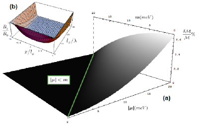
where we have included the electric permittivity $\varepsilon$ and the magnetic permeability $\mu$. To obtain the TME, we apply a magnetic field of magnitude $B_{0}$ perpendicular to the sample . The corresponding boundary conditions are $B_{z}(\pm l_{x})=B_{0}$. The magnetic field satisfies the differential equation $\left(\frac{\partial^{2}}{\partial x^{2}}-\frac{1}{\lambda^{2}}\right)B_{z}^{\phantom{{\dagger}}}=0$, with $\lambda=[(\sqrt{\varepsilon/\mu}\phantom{.})/\sigma_{xy}]d$, the zero temperature penetration depth. This is indeed the equation we find in the case of a superconductor. Notice that in our case only the $z$-component of the magnetic field is involved, implying that the TME takes place only for magnetic fields perpendicular to the plane. Solving the above equation using the aforementioned boundary conditions yields $B_{z}(x)=B_{0}^{\phantom{{\dagger}}}[\cosh(x/\lambda)]/{\cosh(l_{x}/\lambda)}$. In Fig.(1b) we plot the magnetic field versus the ratio of $l_{x}/\lambda$ throughout the whole sample. For $l_{x}>>\lambda$ we have almost complete screening of the magnetic field. Integration of $B_{z}$ over the whole sample yields the magnetization ${\cal M}={\cal M}_{0}^{\phantom{{\dagger}}}[\tanh\left({l_{x}^{\phantom{{\dagger}}}}/{\lambda}\right)]/\left({l_{x}^{\phantom{{\dagger}}}}/{\lambda}\right)$, where we have introduced the zero temperature magnetization ${\cal M}_{0}=B_{0}L_{x}L_{y}$, corresponding to full penetration. One can readily obtain the dependence of the magnetization on the chemical potential in the $l_{x}^{\phantom{{\dagger}}}>>\lambda$ regime. Using Eq.(5), we find ${\cal M(\mu)}\simeq{\cal M}_{0}\lambda(\mu)/l_{x}^{\phantom{{\dagger}}}={\cal M}/(1-n_{ex})$ and $\delta{\cal M}/{\cal M}=n_{ex}/(1-n_{ex})$. As shown in Fig.(1a), the relative change of the magnetization due to doping is unimportant for low doping, where it stands $\delta{\cal M}/{\cal M}\simeq n_{ex}\sim\mu^{2}/t\Delta$.

Figure 2: (Color online) Magnetization ratio ${\cal M}/{\cal M}_{0}$ versus temperature $T$ for different values of the ratio $l_{x}/\lambda$. For $T<T_{onset}$ the system is in a chiral d-density wave state. In a BCS approximation, these curves are identical to the superconducting case.

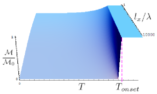
We may also obtain the temperature dependence of the magnetization by assuming that the penetration depth has the usual BCS temperature dependence $[\lambda/\lambda(T)]^{2}={1-\left({T}/{T_{onset}}\right)^{4}}$. Under this consideration, we obtain the magnetization curves shown in Fig.(2) which are identical to the ones encountered in the superconducting case as expected within this BCS treatment. If we compare the magnetization curves of Fig.(2) with the experimental results in the cuprates, we observe that our BCS approximation does not provide a fully satisfactory fit. Nonetheless, a strict quantitative comparison calls for an implementation of our picture, that would be more adapted to the cuprate materials.

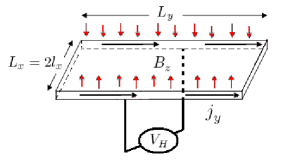
A direct experimental verification of the presence of a CDDW could be provided by the SQHE (Fig.(3)). If a CDDW is present, a Hall voltage can be generated by the sole application of a magnetic field. Specifically, we solve Eq.(9) with boundary conditions $E_{x}(\pm l_{x})=0$ and $B(\pm l_{x})=\pm B_{0}$, as in Ref.Furusaki . The spontaneously generated Hall voltage is, $V_{H}=vB_{0}L_{x}\left[\coth\left({l_{x}}/{\lambda}\right)-{\lambda}/{l_{x}}\right],$ where $v=1/\sqrt{\mu\varepsilon}$ is the velocity of light in the material. If $\l_{x}>>\lambda$, $V_{H}^{\phantom{{\dagger}}}=vB_{0}^{\phantom{{\dagger}}}L_{x}^{\phantom{{\dagger}}}$, which implies that the applied magnetic field totally transforms to an electric field. However, if there is a number of domains of different chiralities in the sample, the SQHE is not an efficient probe of the CDDW. Nevertheless, there is an alternative route in detecting a CDDW. We refer to the gapless chiral edge modes that exist on the boundary surfaces separating the bulk from the vacuum. In order to restore the gauge invariance of the Chern-Simons terms, these current carrying modes appear, constituting a direct indication of a CDDW Furusaki ; Horovitz .

Figure 3: (Color online) Spontaneous Quantum Hall Effect as a signature of the chiral d-density wave. Symmetrical surface currents running along the y-axis create a magnetic field distribution $B(\pm l_{x})=\pm B_{0}$ leading to the spontaneous generation of a Hall voltage $V_{H}$.

Based on the ${\cal P-T}$ violation and the possibility of a spontaneous electric Hall response via the SQHE we naturally expect a CDDW to exhibit a spontaneous thermoelectric Hall response Zhang , detectable in principle, in a Nernst measurement. The unusual Nernst contribution has the same origin with the TME and consequently they should scale. This implies that the simultaneous presence of both enhanced Nernst and diamagnetic signals reported in the pseudogap regime is compatible with the assumption of a CDDW state.

In conclusion, we have proposed an alternative way of generating a Meissner effect without invoking in any manner superconductivity. In our picture, the existence of a chiral d-density wave (CDDW) generates the Topological Meissner effect (TME) due to ${\cal P-T}$ violation. The direction of the chirality of the CDDW guarantees that the TME takes place only for perpendicular to the plane magnetic fields, which is in agreement with the diamagnetic observations in the pseudogap regime of the cuprates. Moreover, a spontaneous thermoelectric response that accompanies the TME is consistent with the observed unusual Nernst signal. Note also, that the presence of a CDDW is compatible with the recently observed quantum oscillations in YBCO quantum oscillations that reported Fermi surface pockets in the nodal areas, possibly indicating the doubling of the Brillouin zone. As a matter of fact, associating a CDDW with the pseudogap regime seems quite promising and undoubtedly further theoretical investigation should be performed.

We are grateful to Professors P. B. Littlewood, N. P. Ong, V.M. Yakovenko, M. Sigrist and P. Thalmeier for stimulating and enlightening comments and discussions. We acknowledge financial support by the EU through the STRP NMP4-CT-2005-517039 CoMePhS. One of the authors (P.K.) also acknowledges financial support by the Greek Scholarships State Foundation.

References

- (1) See e.g. J. R. Schrieffer, Theory of Superconductivity, The Benjamin/Cummings Publishing Company (1983).
- (2) Yayu Wang, Lu Li, and N. P. Ong, Phys. Rev. B 73, 024510 (2006); Yayu Wang, Lu Li, M. J. Naughton, G. D. Gu, S. Uchida, and N. P. Ong, Phys. Rev. Lett. 95, 247002 (2005); Lu Li, Yayu Wang, M. J. Naughton, S. Ono, Yoichi Ando, and N. P. Ong, Europhys. Lett. 72, 451 (2005); N. P. Ong, Yayu Wang, S. Ono, Yoichi Ando, and S. Uchida, Ann. Phys. (Leipzig) 13, 9 (2004); U. Thisted, J. Nyhus, T. Suzuki, J. Hori, and K. Fossheim, Phys. Rev. B 67, 184510 (2003).
- (3) T. Timusk and B. Stratt, Rep. Prog. Phys. 62, 61 (1999); P.A. Lee, N. Nagaosa and X-G. Wen, Rev. Mod. Phys. 78, 17 (2006); E. W. Carlson, V. J. Emery, S. A. Kivelson, and D. Orgad, cond-mat/0206217.
- (4) S. Chakravarty, R. B. Laughlin, D. K. Morr, and C. Nayak, Phys. Rev. B 63, 094503 (2001).
- (5) Other states similar to the DDW have been proposed by: I. Affleck and J. B. Marston, Phys. Rev. B 37, 3774 (1988); X. G. Wen and P. A. Lee, Phys. Rev. Lett. 76, 503 (1996); C. M. Varma, Phys. Rev. Lett. 83, 3538 (1999).
- (6) H. J. Schulz, Phys. Rev. B 39, 2940 (1989); P. Thalmeier, Z. Phys. B 100, 387 (1996); C. Nayak, Phys. Rev. B 62, 4880 (2000).
- (7) A. A. Nersesyan and G. E. Vachnadze, J. Low Temp. Phys. 77, 293 (1989). A DDW can show, under circumstances, a diamagnetic response due to Landau level formation but not a true Meissner effect.
- (8) V. J. Emery and S. A. Kivelson, Nature (London) 374, 434 (1995).
- (9) J. M. Kosterlitz and D. J. Thouless, J. Phys. C 6, 1181 (1973); M. R. Beasley, J. E. Mooij, and T. P. Orlando, Phys. Rev. Lett. 42, 1165 (1979).
- (10) A. Damascelli, Z. Hussain, and Z.-X. Shen, Rev. Mod. Phys. 75, 473 (2003).
- (11) Kenjiro K. Gomes, A. N. Pasupathy, A. Pushp, S. Ono, Yoichi Ando, and A. Yazdani, Nature 447, 569-5720 (2007).
- (12) P. Kotetes and G. Varelogiannis, Europhys. Lett., 84, 37012 (2008).
- (13) V. M. Yakovenko, Phys. Rev. Lett. 65, 251 (1990).
- (14) J. Froehlich and T. Kerler, Nucl. Phys. B 354, 369 (1991).
- (15) J. Goryo and K. Ishikawa, Phys. Lett. A 246, 549 (1998); 260, 294 (1999).
- (16) A. Furusaki, M. Matsumoto, and M. Sigrist, Phys. Rev. B 64, 054514 (2001).
- (17) B. Horovitz and A. Golub, Phys. Rev. B 68, 214503 (2003).
- (18) G. E. Volovik, The Universe in a Helium Droplet, Oxford Science Publications (2003).
- (19) G. W. Semenoff, Phys. Rev. Lett. 53, 2449 (1984); F. D. M. Haldane, Phys. Rev. Lett. 61, 2015 (1988).
- (20) S. Deser, R. Jackiw and S. Templeton, Phys. Rev. Lett. 48, 975 (1982); Ann. Phys. (NY) 140, 372 (1982).
- (21) E. Fradkin, Field Theories of condensed matter systems, Addison Wesley (1991).
- (22) S. Tewari, C. Zhang, V. M. Yakovenko, and S. Das Sarma, Phys. Rev. Lett. 100, 217004 (2008).
- (23) J. Xia, E. Schemm, G. Deutscher, S. A. Kivelson, D. A. Bonn, W. N. Hardy, R. Liang, W. Siemons, G. Koster, M. M. Fejer, and A. Kapitulnik, Phys. Rev. Lett. 100, 127002 (2008).
- (24) X.G. Wen, Phys. Rev. B 43, 11025 (1991); N. Maeda, Phys. Rev. B 376, 142 (1996).
- (25) C. Zhang, S. Tewari, V. M. Yakovenko, and S. Das Sarma, cond-mat/0803.3220.
- (26) E. A. Yelland, J. Singleton, C. H. Mielke, N. Harrison, F. F. Balakirev, B. Dabrowski, and J. R. Cooper, Phys. Rev. Lett. 100, 047003 (2008); A. F. Bangura, J. D. Fletcher, A. Carrington, J. Levallois, M. Nardone, B. Vignolle, P. J. Heard, N. Doiron-Leyraud, D. LeBoeuf, L. Taillefer, S. Adachi, C. Proust, and N. E. Hussey, Phys. Rev. Lett. 100, 047004 (2008).