MZ-TH/07-22


Determination of QCD condensates
from $\tau$-decay data

Abstract

We have used the latest data from the ALEPH Collaboration to extract values for QCD condensates up to dimension $d=12$ in the $V-A$ channel and up to dimension $d=8$ in the $V$, $A$ and $V+A$ channels. Performing 2- and 3-parameter fits, we obtain new results for the correlations of condensates. The results are consistent among themselves and agree with most of the previous results found in the literature.

1 Introduction

QCD is widely considered to be a good candidate for a theory of the strong interactions. Asymptotic freedom allows us to perform a perturbative treatment of strong interactions at short distances. Long distance behaviour, however, is not fully understood: it is commonly believed that, due to the nontrivial structure of the physical vacuum, the perturbation expansion does not completely define the theory and that one has to add non-perturbative effects as well. In order to make a comparison with experiments possible even in the resonance energy range, Shifman, Vainshtein and Zakharov [1] have proposed to use the Operator Product Expansion (OPE) and to introduce the vacuum expectation values of operators occurring in the OPE, the so called condensates, as phenomenological parameters. It is worth to study these parameters in order to see whether one can indeed obtain a consistent description of the low energy hadronic physics and get more insight into the properties of the QCD vacuum. It is, in particular, important to determine the range of values of the condensates allowed by presently available experimental data.

Condensates are needed in the description of two-point functions of hadronic currents: together with the results of perturbative QCD they allow us to obtain approximate theoretical predictions for the hadronic current correlators in the space-like region. On the other hand, in the time-like region, the discontinuity of these amplitudes is directly related to measurable quantities. Analyticity strongly correlates the energy dependence of the amplitudes in these two regions; however, due to errors affecting both the theoretical predictions as well as the experimental data, the relation of the two-point functions in the time-like and space-like regions must be carefully analysed before it can be used in applications.

There are several methods, generically called QCD sum rules [1, 2, 3], that have been used in the past for obtaining values of the QCD condensates. They all rely implicitly on the assumption that an analytic extrapolation from the time-like to the space-like region is possible without introducing additional uncertainties. Therefore they can include theoretical errors in the space-like region only at a qualitative level, and/or need (explicit and implicit) assumptions on the derivatives of the amplitudes. A quantitative estimate of the errors including both experimental and theoretical ones (truncation of the perturbative and operator product expansions) is therefore very difficult in these approaches. The application of fully controlled analytic extrapolation techniques should remedy these effects. There are a few methods of this sort, in which the error channels in the space-like region are defined through $L^{2}$-norms [4, 5] or $L^{\infty}$-norms [6, 7, 8].

The functional method that we have developed and used in a previous publication for an analysis of the correlator of the $V-A$ current [4], allows us to extract within rather general assumptions the condensates from a comparison of the time-like experimental data with the asymptotic space-like results from theory. We will see that the price to be paid for the generality of assumptions is relatively large errors in the values of the extracted parameters. In this respect, our method is not superior to other approaches; however, we hope that our results provide additional confidence in the numerical results obtained with the help of methods based on QCD sum rules [1, 2, 3, 9, 10, 11].

The paper is organised as follows: In the first section the theoretical aspects of hadronic $\tau$-decays are considered while in section 3 we describe the experimental data at hand. The actual method used to extract the condensates is presented in section 4. Basically the method is the one reported in [4] but here a generalisation to all channels is performed. The results are summarised in section 5. We quote results in all the four channels where data are available. Results for the $V-A$ channel were already published in [4]; for completeness, we repeat those previous results in the present paper and extend our analysis by a new 3-parameter fit. New results were obtained in the $V$, $A$ and $V+A$ channels from 1-, 2- and 3-parameter fits. We shall also discuss important consistency checks of our method in section 6. The comparison of our findings with others present in the literature is performed in section 7.

2 Theoretical description of hadronic $\tau$-decays

The $\tau$ lepton is heavy enough ($m_{\tau}=1.777$ GeV) to decay not only into other leptons, but into final states involving hadrons as well. These decays offer an ideal laboratory for the study of strong interactions, including the transition from the perturbative to the non-perturbative regime of QCD in the simplest possible reaction. This might explain the tremendous efforts ongoing in both theoretical and experimental studies of $\tau$ physics.

We consider the correlator of hadronic vector and axial-vector charged currents, $J_{\mu}=V_{\mu}=\bar{u}\gamma_{\mu}d$ and $J_{\mu}=A_{\mu}=\bar{u}\gamma_{\mu}\gamma_{5}d$,

$$\Pi_{\mu\nu}^{J} = i\int d^{4}xe^{iqx}\langle TJ_{\mu}(x)J_{\nu}(0)^{\dagger}\rangle$$

$$= \left(-g_{\mu\nu}q^{2}+q_{\mu}q_{\nu}\right)\Pi_{J}^{(0+1)}(q^{2})+g_{\mu\nu}q^{2}\Pi_{J}^{(0)}(q^{2})\,.$$

The conservation of the vector current implies $\Pi_{V}^{(0)}=0$. The connection to experimental observables is most easily expressed with the help of the spectral functions which are related to the absorptive part of the correlators. Using the normalisation as defined in most of the previous publications, the functions

$$v_{j}(s)=2\pi{\rm Im}\Pi_{V}^{(j)}(s),~{}~{}~{}~{}a_{j}(s)=2\pi{\rm Im}\Pi_{A}^{(j)}(s)$$ (2)

can be extracted from the decay spectrum of hadronic $\tau$-decays.

The hadronic polarisation tensor can be rewritten using the OPE:

$$\Pi^{(j)}_{V,A}(s)=\sum_{d\geq 0}\frac{{\cal O}_{d}^{(j),{V,A}}}{(-s)^{d/2}},$$ (3)

where ${\cal O}_{d}\equiv{\cal C}_{d}\langle{\cal O}_{d}\rangle$ is the short hand notation for the QCD non-perturbative condensate $\langle{\cal O}_{d}\rangle$ of dimension $d$ and its associated perturbative Wilson coefficient ${\cal C}_{d}$; $s\equiv q^{2}$ is the squared momentum transfer.

The contribution to (3) of lowest dimension, $d=0$, is entirely given by perturbation theory. For that reason it is useful to separate the two contributions in (3):

$$\Pi^{(j)}_{V,A}(s)=\Pi_{{\rm PT},V,A}^{(j)}(s)+\Pi_{{\rm OPE},V,A}^{(j)}(s).$$ (4)

As will become clear when we describe our method (section 4) it is enough to consider the first derivative of the perturbative part, i.e., the Adler function

$$D(s)\equiv-s\frac{d}{ds}\Pi_{\rm PT}(s),$$ (5)

which is known in the massless-quark limit up to terms of order $\alpha_{s}^{4}$. After re-summing the leading logarithms it reads, for space-like momenta ($s<0$):

$$D_{V,A}(s)=\frac{1}{4\pi^{2}}\sum_{n\geq 0}^{4}\ K_{n}\left(\frac{\alpha_{s}(-s)}{\pi}\right)^{n}.$$ (6)

The coefficients $K_{n}$ are the same for both $V$ and $A$ channels. For 3 flavours, in $\overline{\rm MS}$ regularisation, $K_{0}=K_{1}=1$, $K_{2}=1.64$ [12, 13, 14], $K_{3}=6.37$ [15, 16] and for $K_{4}$ there are two estimates $K_{4}=25\pm 25$ [17] and $K_{4}=27\pm 16$ [18].

For the correlators with spin $0+1$ and in the chiral limit, the non-perturbative part has the form

$$\Pi^{(0+1)}_{{\rm OPE},V,A}(s)=\sum_{d\geq 4}\frac{{\cal O}_{d}^{V,A}}{(-s)^{d/2}}\left(1+c_{d}^{{\rm NLO},V,A}\frac{\alpha_{s}(\mu^{2})}{\pi}\right),$$ (7)

where perturbative corrections of order $O(\alpha_{s})$ are taken into account, described by coefficients $c_{d}^{\rm NLO}$. Some of the NLO coefficients were calculated in [19, 20, 21].

The parameters ${\cal O}_{d}$ can be related to vacuum expectation values of products of quark and gluon field operators [1]. Often vacuum dominance or the factorization approximation, which holds, e.g., in the large-$N_{c}$ limit, is assumed. Our analysis does not rely on such a representation.

3 Experimental data

Since its discovery, the $\tau$ lepton has been studied with ever-increasing precision at every new $e^{+}e^{-}$ collider that has gone into operation. We are particularly interested in the comprehensive measurements of exclusive hadronic branching ratios from ALEPH [22, 23] and of the non-strange spectral functions from ALEPH [22, 23] and OPAL [24] that have yielded important contributions to studies of perturbative QCD at low energies and, in particular, to the measurement of $\alpha_{s}(m_{\tau}^{2})$. Recent measurements of a set of semi-exclusive branching ratios by DELPHI are also available [25], but have not been analyzed to a similar extent. A number of exclusive branching ratio measurements from BaBar have been reported already [26] and with more work invested in the understanding of these higher-multiplicity final states we may expect high-precision data for the spectral functions to come also from the B-factories.

We have chosen to use the final data from the ALEPH collaboration [23] because, as compared to those available from OPAL [24], they have the smallest experimental errors and provide a larger number of bins.

The spectral functions (2) are obtained by dividing the normalised invariant mass-squared distribution of hadronic $\tau$ decays, $dR_{\tau,{V,A}}/ds$, for a given hadronic mass $\sqrt{s}$ by the appropriate kinematic factor. They are then normalised to the branching fraction of the massless leptonic, i.e. electron, channel ${\cal B}_{e}=(17.810\pm 0.039)\%$ [23]:

$$\begin{array}[]{r}\displaystyle v_{1}(s)=\frac{m_{\tau}^{2}}{6|V_{ud}|^{2}S_{\rm EW}}\frac{dR_{\tau,{V}}}{{\cal B}_{e}ds}\left[\left(1-\frac{2}{m_{\tau}^{2}}\right)^{2}\left(1+2\frac{s}{m_{\tau}^{2}}\right)\right]^{-1},\\ \\ \displaystyle a_{1}(s)=\frac{m_{\tau}^{2}}{6|V_{ud}|^{2}S_{\rm EW}}\frac{dR_{\tau,{A}}}{{\cal B}_{e}ds}\left[\left(1-\frac{2}{m_{\tau}^{2}}\right)^{2}\left(1+2\frac{s}{m_{\tau}^{2}}\right)\right]^{-1},\\ \\ \displaystyle a_{0}(s)=\frac{m_{\tau}^{2}}{6|V_{ud}|^{2}S_{\rm EW}}\frac{dR_{\tau,{A}}}{{\cal B}_{e}ds}\left(1-\frac{2}{m_{\tau}^{2}}\right)^{-2}.\end{array}$$ (8)

Here $S_{\rm EW}=1.0198\pm 0.0006$ accounts for short distance electroweak radiative corrections [27] and the CKM mixing matrix element has the value $|V_{ud}|=0.9746\pm 0.0006$ [28]. Due to the conservation of the vector current, there is no $j=0$ contribution to the vector spectral function, while the only contribution to $a_{0}$ is assumed to come from the pion pole. The spectral function $a_{0}$ is connected, via partial conservation of the axial-vector current (PCAC), to the pion decay constant $f_{\pi}=0.1307\mbox{ GeV}$ [29] through $a_{0,\pi}(s)=2\pi^{2}f_{\pi}^{2}\delta(s-m_{\pi}^{2})$.

4 The determination of condensates: a functional method

Let us consider a set of functions $F(s)$ which are admissible as a representation of the true correlator if they are real analytic functions in the complex $s$-plane cut along the time-like interval $[s_{0},\infty)$ with $s_{0}>0$. The asymptotic behaviour of $F(s)$ is restricted by fixing the number of subtractions in the dispersion relation between $F(s)$ and its imaginary part $f(s)=\mbox{Im}F(s+i0)$ along the cut:

$$F(s)=\frac{1}{\pi}\int_{s_{0}}^{\infty}\frac{f(z)dz}{z-s}+\mbox{subtractions}\ .$$ (9)

For our purpose it is convenient to get rid of the subtraction terms by taking an appropriate number of derivatives with respect $s$. We denote by ${\cal C}_{n}(s,z)$ the kernel occurring in the dispersion relation for the $n$-th derivative of $F(s)$:

$$-s^{n}F^{(n)}(s)=\frac{1}{\pi}\int_{s_{0}}^{\infty}{\cal C}_{n}(s,z)f(z)dz\ .$$ (10)

For example, in the special case of the $V-A$ correlator which vanishes identically in the chiral limit to all orders in QCD perturbation theory there are no subtractions needed and thus one takes $n=0$. In this case, the dispersion relation will be identical to the one of Eq. (9) with no subtraction terms. On the other hand, the $V$, $A$ and $V+A$ correlators are dominated by their perturbative contributions and there is one subtraction needed in the dispersion relation. To get rid of this usually unknown constant term one needs to take the first derivative and set $n=1$.

In order to determine $F(s)$ and $f(s)$ we use the following two available sources of information:

• experimental data measured in the time-like interval $\Gamma_{\rm exp}=[s_{0},s_{\rm max}]$:

  $$f_{\rm exp}(s)=\frac{1}{2\pi}\left\{\begin{array}[]{ll}v_{1}(s),&\mbox{in the}\ V\ \mbox{channel,}\\ a_{1}(s)+a_{0}(s),&\mbox{in the}\ A\ \mbox{channel.}\end{array}\right.$$ (11)

  The extension to $V\pm A$ channels is straightforward.

• theoretical model given by perturbative QCD, i.e.,

  • the prediction for $F(s)$ in the space-like interval $\Gamma_{L}=[s_{2},s_{1}]$:

    $$F_{\rm QCD}(s)\equiv\Pi^{(0+1)}_{J}(s),\quad J=V,~{}A,~{}V+A,~{}V-A$$ (12)

  • and $\left.f_{\rm QCD}(s)=\mbox{Im}F_{\rm QCD}(s+i0)\right|_{s\in(s_{\rm max},\infty)}$ since QCD is expected to be reliable for large energies.

As a next step in extracting values for the condensates, we split the integral on the r.h.s. of the modified dispersion relation (10) into two parts: one that can be described by the experiment and the other one by the theoretical model, i.e., QCD:

$$\underbrace{-s^{n}F^{(n)}_{\rm QCD}(s)-\frac{1}{\pi}\int_{s_{\rm max}}^{\infty}{\cal C}_{n}(s,z)f_{\rm QCD}(z)dz}=\underbrace{\frac{1}{\pi}\int_{s_{0}}^{s_{\rm max}}{\cal C}_{n}(s,z)f(z)dz}.$$ (13)

QCD prediction: ${\tilde{F}}^{n}_{\rm QCD}(s)$                     experimental data

The goal of the method is to check if there exists a function $F(s)$ which is in accord with both the data on $\Gamma_{\rm exp}$ and the model on $\Gamma_{L}$. For doing this, one can use an $L^{2}$-norm approach and define two functionals $\chi_{L}^{2}[f]$ and $\chi_{R}^{2}[f]$. $\chi_{R}^{2}[f]$ compares the true amplitude $f(s)$ with the data. Here one can take into account not only experimental errors on each individual bin, but the full correlation of available data by using the covariance matrix $V$ provided by ALEPH as a weight function. Therefore we define

$$\chi^{2}_{R}[f]=\frac{1}{|\Gamma_{\rm exp}|}\int_{s_{0}}^{s_{\rm max}}dx\int_{s_{0}}^{s_{\rm max}}dx^{\prime}V^{-1}(x,x^{\prime})(f(x)-f_{\rm exp}(x))(f(x^{\prime})-f_{\rm exp}(x^{\prime})).$$ (14)

As a measure for the agreement of the true function $f(s)$ with the theory, we define $\chi_{L}^{2}[f]$ by comparing the left and right hand sides of (13)

$$\chi^{2}_{L}[f]=\displaystyle\frac{1}{|\Gamma_{L}|}\int_{\Gamma_{L}}w_{L}(x)\left({\tilde{F}}^{n}_{\rm QCD}(x)-\displaystyle\frac{1}{\pi}\int_{s_{0}}^{s_{\rm max}}{\cal C}_{n}(x,x^{\prime})f(x^{\prime})dx^{\prime}\right)^{2}dx,$$ (15)

where $w_{L}$ is a weight function for the space-like interval, i.e. an a-priori estimate of the accuracy of the QCD predictions, and written as $1/\sigma_{L}^{2}(s)$. $\sigma_{L}(s)$ should be chosen as a continuous, strictly positive function of $s\in\Gamma_{L}$ and encodes errors due to the truncation of the perturbative series and the OPE. It is expected to decrease as $|s|\rightarrow\infty$ and diverge for $s\rightarrow 0$. For example, in the case of the $V-A$ correlator we will use the next higher dimension contribution in the OPE as an error estimate on the space-like region. In the case of the $V$, $A$ and $V+A$ correlators the situation is a bit more complicated since they are dominated by their perturbative part. Thus one has three possibilities to define an error corridor: one can use the last known term of the perturbation series, or the first omitted term in the OPE, or a combination of the two of them. As an illustration, in the case of a 1-parameter fit $\sigma_{L}^{V,A}(s)$ would be given by

$$\sigma_{L}^{V,A}(x)=\left\{\begin{array}[]{ll}\displaystyle\frac{1}{4\pi^{2}}K_{3}\left(\frac{\alpha_{s}(-x)}{\pi}\right)^{3},\\ \\ \displaystyle 3\frac{{\cal O}_{6}^{V,A}}{(-x)^{3}}\,,\\ \\ \displaystyle\sqrt{\left[\frac{1}{4\pi^{2}}K_{3}\left(\frac{\alpha_{s}(-x)}{\pi}\right)^{3}\right]^{2}+\left[3\frac{{\cal O}_{6}^{V,A}}{(-x)^{3}}\right]^{2}}\,.\\ \end{array}\right.$$ (16)

The factor 3 in front of ${\cal O}_{6}^{V,A}$ in the expression of $\sigma_{L}^{V,A}(x)$ comes from the fact that in the $V$, $A$ and $V+A$ channels one needs to set $n=1$ in Eq. (10) and thus take the first derivative of the operator product expansion in Eq. (7). $K_{3}$ was given in section 2.

In order to find the true function $f(s)$ one can combine the information contained in these two functionals by means of Lagrange multipliers and find the unrestricted minimum of

$${\cal F}[f]=\chi^{2}_{L}[f]+\mu\chi^{2}_{R}[f],$$ (17)

subject to the condition

$$\chi_{R}^{2}[f]\leq\chi_{\rm exp}^{2}=\frac{1}{N}\sum_{i,j}\sqrt{V(s_{i},s_{i})V(s_{j},s_{j})}V^{-1}(s_{i},s_{j}),$$ (18)

which will be the criterion to determine the Lagrange multiplier $\mu$. This procedure leads to an integral equation for the imaginary part of the true amplitude, $f(x;\mu)$:

$$\begin{array}[]{r}f(x;\mu)=\displaystyle f_{\rm exp}(x)+\frac{\lambda|\Gamma_{\rm exp}|}{\pi|\Gamma_{L}|}\int_{s_{0}}^{s_{\rm max}}dy\,V(y,x)\int_{\Gamma_{L}}dz\,w_{L}(z){\cal C}_{n}(z,y){\tilde{F}}^{n}_{\rm QCD}(z)\\ \\ +\displaystyle\lambda\int_{s_{0}}^{s_{\rm max}}dz\,{\cal K}(x,z)f(z;\mu),\end{array}$$ (19)

where $\lambda=1/\mu$ and

$${\cal K}(x,z)=-\frac{|\Gamma_{\rm exp}|}{\pi^{2}|\Gamma_{L}|}\int_{s_{0}}^{s_{\rm max}}dy\,V(y,x)\int_{\Gamma_{L}}dx^{\prime}\,w_{L}(x^{\prime}){\cal C}_{n}(x^{\prime},y){\cal C}_{n}(x^{\prime},z).$$ (20)

Thus, the algorithm for determining acceptable values for the condensates is the following [30]:

• Choose a model by stating how many terms in the OPE should be taken into account. The term with the next-highest dimension is used to define an error corridor in the space-like region;

• Solve the integral equation (19) iteratively, with fixed values of the free parameters of the chosen model, until the Lagrange multiplier $\mu$ satisfies the condition (18);

• Calculate $\chi_{L}^{2}$ corresponding to the above solution as a function of the free parameters;

• Minimise $\chi_{L}^{2}$ with respect to variations of the model parameters. The corresponding parameter values are the condensates we are looking for;

• Determine confidence regions around the fitted parameters by solving

  $$\chi_{L}^{2}=\chi_{L,\rm min}^{2}+\Delta\chi^{2}.$$ (21)

  Here we will assume that the underlying probability distribution is Gaussian, fixing $\Delta\chi^{2}$ to reflect the conventional 1-, 2- and $3\sigma$-contours for $n$-parameter fits. Numerical values for errors will be given for $1\sigma$ confidence intervals.

5 Results and discussion

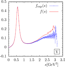
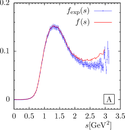
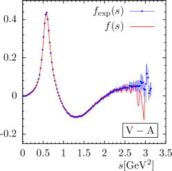
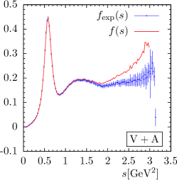
The most important step of our analysis is to find a function $f(s)$ (Eq. (19)) which provides a best fit to both the data and the theoretical model. A direct comparison of the experimental data with the regularised function $f(s)$ obtained from 1-parameter fits is shown in Fig. 1. We find nice agreement over the full range of $s$ with the exception of the highest $s$-bins. Here the spread of data points is apparently wider than individual errors on single data points. The largest differences are visible in the $V+A$ channel at $s>2$ GeV² where the discrepancies in the $V$ and $A$ channels between data and the fitted function $f(s)$ get enhanced while they appear to be compensated in the $V-A$ channel. We emphasize that we have used the full correlation matrix provided by ALEPH. Correlations are certainly important in our fit, however, they can not be visualized in our figure.

Figure 1: The regularised function $f(s)$ (see Eq. (19)) compared to the experimental data of Ref. [23]. $f(s)$ was obtained with 1-parameter fits using the 120 first $s$-bins, i.e. from $s\leq 3$ GeV².

5.1 1-parameter fits

Let us start with 1-parameter fits and quote results for condensates of dimension $d=4$ ($V$, $A$, $V+A$) and $d=6$ ($V-A$) [4]:

$${\cal O}_{4}^{V} = 1.6_{-0.5}^{+0.4}\times 10^{-3}{\rm GeV}^{4},\hskip 28.45274pt\chi_{L,{\rm min}}^{2}=49,$$

$${\cal O}_{4}^{A} = 2.6_{-0.4}^{+0.4}\times 10^{-3}{\rm GeV}^{4},\hskip 28.45274pt\chi_{L,{\rm min}}^{2}=2.8,$$

$${\cal O}_{4}^{V+A} = 4.2_{-0.9}^{+0.8}\times 10^{-3}{\rm GeV}^{4},\hskip 28.45274pt\chi_{L,{\rm min}}^{2}=19,$$

$${\cal O}_{6}^{V-A} = -5.9_{-1.0}^{+1.7}\times 10^{-3}{\rm GeV}^{6},\hskip 19.91692pt\chi_{L,\rm min}^{2}=0.17.$$

In the 1-parameter fits we have fixed all higher-dimension condensates to be zero. The results of the $V-A$ analysis had been given earlier [4]. There we obtained an acceptable fit when choosing an error corridor defined by the dimension $d=8$ condensate in the space-like region with

$$\left|{\cal O}_{8}^{V-A}\right|_{\rm max}\simeq 1.3\times 10^{-3}{\rm GeV^{8}}.$$ (22)

Our fit thus provides an indirect estimate of the upper limit of $|{\cal O}_{8}^{V-A}|$. In the other channels we have used the coefficient $K_{3}$ in the perturbative expansion of the Adler function to define the theory error.

5.2 2-parameter fits

When performing 2-parameter fits we aim to determine simultaneously the first two relevant condensates appearing in the operator product expansion. The additional freedom in the fit provided by the second parameter allows us, in general, to obtain better fits. In fact, it turns out that, except for the $V-A$ channel, the condensates of next-to-lowest dimension have significant non-zero values, in contrast to the assumption underlying the 1-parameter fits.

Figure 2: 2-parameter fits: 1-, 2- and 3$\sigma$ confidence regions defined by contours of constant $\chi_{L}^{2}$ in the plane of the two fitted parameters. The central values (see Tab. 1) are marked by dashed lines.

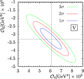
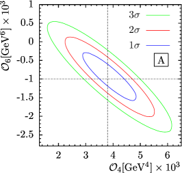
In Fig. 2 we show contours of constant $\chi^{2}_{L}$. One can see that we find strong correlations between the two free parameters. This correlation allows us to determine a linear combination of the two parameters with a well defined and rather small error:

$$\begin{array}[]{l}{\cal O}_{6}^{V}+0.65\mbox{ GeV}^{2}\ {\cal O}_{4}^{V}=0.66_{-0.25}^{+0.25}\times 10^{-3}\mbox{ GeV}^{6},\\ \\ {\cal O}_{6}^{A}+0.65\mbox{ GeV}^{2}\ {\cal O}_{4}^{A}=1.60_{-0.25}^{+0.26}\times 10^{-3}\mbox{ GeV}^{6},\\ \\ {\cal O}_{6}^{V+A}+0.65\mbox{ GeV}^{2}\ {\cal O}_{4}^{V+A}=2.20_{-0.51}^{+0.50}\times 10^{-3}\mbox{ GeV}^{6},\\ \\ {\cal O}_{8}^{V-A}+2.22\mbox{ GeV}^{2}\ {\cal O}_{6}^{V-A}=-18.30_{-0.25}^{+0.38}\times 10^{-3}\mbox{ GeV}^{8}.\end{array}$$ (23)

The location of the minima, i.e. the central values of the fitted parameters are quoted in Tab. 1. As expected, the value of ${\cal O}_{8}^{V-A}$ found in the 2-parameter fit has the same order of magnitude as the corresponding estimate found from the 1-parameter fit (see Eq. 22). Similarly to the 1-parameter fit, we can now give an estimated upper limit of the $V-A$ condensate of dimension $d=10$ which was used in the 2-parameter fit to define the error channel:

$$\left|{\cal O}_{10}^{V-A}\right|_{\rm max}\simeq 5.7\times 10^{-3}{\rm GeV^{10}}.$$ (24)

As before, the error corridors for the $V$, $A$ and $V+A$ channels were defined by the perturbative contribution of order $\alpha_{s}^{3}$ (Eq. 16).

	$V$	$A$	$V+A$	$V-A$
$d=4$	$6.1_{-1.1}^{+0.9}$	$3.8_{-0.9}^{+1.1}$	$9.9_{-2.0}^{+2.1}$
$d=6$	$-3.3_{-0.6}^{+0.7}$	$-1.0_{-0.7}^{+0.6}$	$-4.2_{-1.3}^{+1.3}$	$-6.8_{-0.8}^{+2.0}$
$d=8$				$3.2_{-9.2}^{+2.8}$
$\chi_{L,\rm min}^{2}$	20.4	0.47	7.1	0.37

Table 1: 2-parameter fits: central values of the fitted parameters in units of $10^{-3}{\rm GeV}^{d}$ and the corresponding values of $\chi_{L,\rm min}^{2}$. In the $V$, $A$ and $V+A$ channels the fitted parameters were the condensates of dimension $d=4$ and $6$ while in the $V-A$ channel we have fitted the dimension $d=6$ and $8$ condensates.

Despite of the poor agreement of theory with data in the $V$ and $V+A$ channels, reflected by the large $\chi^{2}_{L,min}$ values, it is important to remark that a consistent over-all picture has emerged from our fits. The results of the 2-parameter fits are in agreement with those from the 1-parameter fit. However, since here the values of ${\cal O}^{V,A,V+A}_{6}$ and ${\cal O}^{V-A}_{8}$ were left unconstrained, we have found larger ranges for ${\cal O}^{V,A,V+A}_{4}$ and ${\cal O}^{V-A}_{6}$. Note in particular that the slope of the correlations in the $V$, $A$ and $V+A$ channels is the same. For the $V+A$ case, the values for both condensates of dimension $d=4$ and $d=6$ agree with the values found by actually taking the sum of the results from the $V$ and $A$ channels.

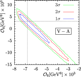
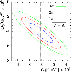
5.3 3-parameter fits

Figure 3: 3-parameter fits in the $V$ and $A$ channels: 1-, 2- and 3$\sigma$ confidence regions defined by contours of constant $\chi_{L}^{2}$ in the plane of two of the fitted parameters and located at the central value of the third one. The central values (see Tab. 2) are marked by dashed lines.

Figure 4: 3-parameter fits in the $V-A$ and $V+A$ channels: 1-, 2- and 3$\sigma$ confidence regions defined by contours of constant $\chi_{L}^{2}$ in the plane of two of the fitted parameters and located at the central value of the third one. The central values (see Tab. 2) are marked by dashed lines.

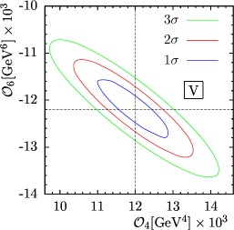
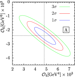
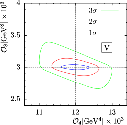
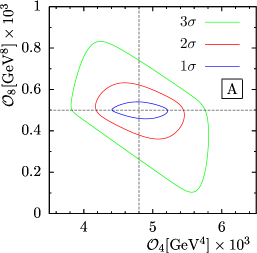
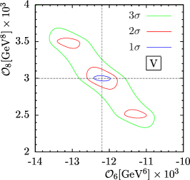
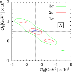
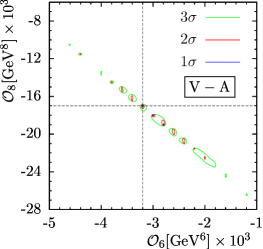
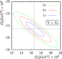
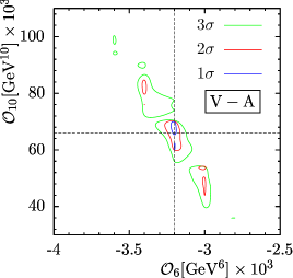
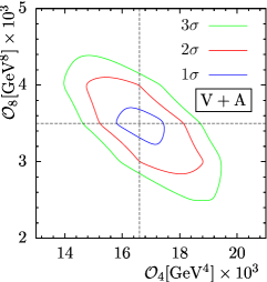
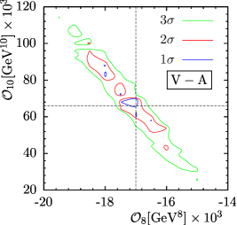
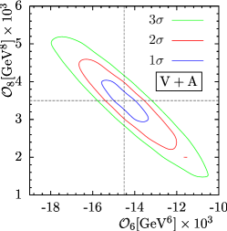
A 3-parameter fit is also possible, where we consider as free parameters the first three relevant condensates in the OPE. We have chosen to display our results as $\chi_{L}^{2}$-contours in the planes defined by the three possible pairs of fit parameters. These correlations are shown in Fig. 3 for the $V$ and $A$ channels and in Fig. 4 for the $V\pm A$ channels. In every case we display 2-dimensional slices of the 3-dimensional allowed parameter ranges keeping the third parameter at its central value as obtained from the 3-parameter fit. These central values are summarised in Tab. 2.

	$V$	$A$	$V+A$	$V-A$
$d=4$	$12.0_{-1.8}^{+1.6}$	$4.8_{-1.8}^{+1.8}$	$16.6_{-3.8}^{+3.2}$
$d=6$	$-12.2_{-1.8}^{+2.0}$	$-2.4_{-2.0}^{+2.0}$	$-14.5_{-4.5}^{+5.0}$	$-3.2_{-0.4}^{+1.6}$
$d=8$	$3.0_{-0.5}^{+0.5}$	$0.5_{-0.5}^{+0.5}$	$3.5_{-1.5}^{+1.5}$	$-17.0_{-9.5}^{+2.5}$
$d=10$				$66.0_{-14.0}^{+40.0}$
$\chi_{L,\rm min}^{2}$	7.15	0.17	2.51	0.35

Table 2: 3-parameter fits: central values of the fitted parameters in units of $10^{-3}{\rm GeV}^{d}$ and their corresponding values of $\chi_{L,\rm min}^{2}$. In the $V$, $A$ and $V+A$ channels the fitted parameters were the condensates of dimension $d=4,\ 6$ and $8$, while in the $V-A$ channel we have fitted the dimension $d=6,\ 8$ and $10$ condensates. The error estimates are obtained by projecting the 3-dimensional ranges allowed by the fit onto the corresponding selected parameter.

An estimated upper limit of the dimension $d=12$ condensate in the $V-A$ channel, the one used to define the error corridor, is

$$\left|{\cal O}_{12}^{V-A}\right|_{\rm max}\simeq 47\times 10^{-3}{\rm GeV^{12}}$$ (25)

which is the expected order of magnitude.

Again we observe that 3-parameter fits turn out to provide better $\chi^{2}_{L,min}$ values than the 2-parameter fits. Obviously, the improved results are obtained since the higher-dimension condensate can be chosen non-zero in the fit. As a consequence, the central values of all condensates are shifted. In addition we observe that the 3-dimensional contours are not always ellipsoids and non-Gaussian errors play a role.

6 Consistency checks

Figure 5: Dependence on the number of data points. $N$ denotes the number of the highest data bin used in the analysis.

In the following we present additional details of our algorithm and describe a number of consistency checks. We have, in particular, studied the behaviour of the algorithm and its results with respect to variations of parameters appearing in the analysis: the number of experimental data points $N$ used for the extraction of condensates, the end-points of the time-like interval $\Gamma_{L}$, $s_{1}$ and $s_{2}$, as well as the dependence on the error parameter needed to define $\sigma_{L}$. In this section, we restrict ourselves to the case of 1-parameter fits.

Figure 6: Dependence on the lower end, $s_{2}$, of the space-like interval: the fitted parameter as a function of $s_{2}$ (left) and $\chi_{L,{\rm min}}^{2}$ as a function of $s_{2}$ (right).

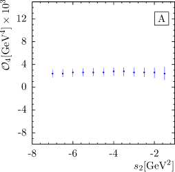
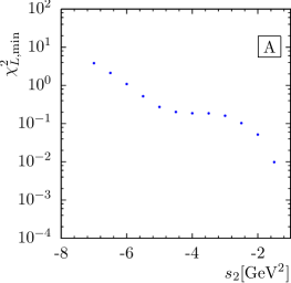
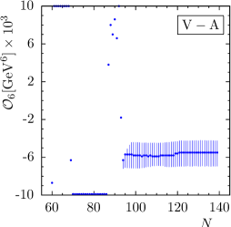
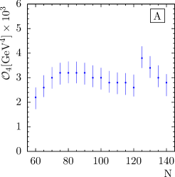
One can show that the information on the condensates is contained in the lower part of the spectrum by adding or removing data points at largest $s$. In Fig. 5 (left panel) we show how the fit result for ${\cal O}_{6}^{V-A}$ depends on the number of data points. One can observe a fast stabilisation of the result already for the $N\simeq 100$ lowest-$s$ data points. In contrast, for the case of the $A$-correlator, cf. Fig. 5 (right panel), one can observe that including or excluding data points above $N=120$ has a stronger effect on the condensate ${\cal O}_{4}^{A}$. In this region the rapid oscillation of the data points as well as large experimental errors play an important role. The decision not to include experimental results from the highest bins in the analysis, is supported by inspecting Fig. 1: there we found that the regularised function obtained in our analysis does not describe the data in the large-$s$ region. We have thus decided to cut off data points above $s=3$ GeV², i.e., we use only the $N=120$ first data points.

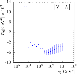
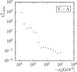
Figure 6 shows the behaviour of the algorithm with respect to changes of $s_{2}$, the lower limit of the space-like interval $\Gamma_{L}$. One should choose $|s_{2}|$ as large as possible, but we observe stability of the algorithm for values certainly not larger than a few times $10^{2}$ GeV² for the $V-A$ analysis and even smaller values are required for the fits of the $A$ condensate. This is illustrated in the right column of Fig. 6 which shows the dependence of $\chi^{2}_{L,\rm min}$ on $s_{2}$. One can observe a plateau for the values of ${\cal O}_{6}^{V-A}$ and ${\cal O}_{4}^{A}$ as a function of $s_{2}$ and thus infer the values used in the analysis to be $s_{2}=-150$ GeV² for $V-A$ and $s_{2}=-3.5$ GeV² for the $A$ channel. For larger values of $|s_{2}|$ the minimum of $\chi_{L}^{2}$ becomes larger than 1, signaling a bad fit. This behaviour may be due to numerical instabilities and limitations of experimental data; more important, however, is the fact that in our LO analysis we did not take into account perturbative higher-order corrections: the large perturbative tails of the $V$- and $A$-correlators become increasingly important when increasing $|s_{2}|$ and the sensitivity to the low-energy condensates is lost.

Figure 7: Dependence on $s_{1}$, the upper limit of the space-like interval $\Gamma_{L}$ for ${\cal O}_{6}^{V-A}$.

In the case of the $A$-correlator, when studying the dependence on $s_{2}$, we found that the best simultaneous description of experimental data and theory is obtained when we choose to define the error corridor with the help of the last known term in the perturbation series, i.e.,

$$\sigma_{L}^{A}(x)=\displaystyle\frac{1}{4\pi^{2}}K_{3}\left(\frac{\alpha_{s}(-x)}{\pi}\right)^{3}.$$ (26)

In contrast, for an error corridor calculated from the next-higher term in the OPE, i.e., using $\sigma_{L}^{A}(s)=\mbox{const}/s^{d}$, we observe a less distinct plateau when varying $s_{2}$ and no stability for the results for ${\cal O}_{4}^{A}$. The fact that with the choice (26) we find very stable fit results for ${\cal O}_{4}^{A}$ even when increasing $|s_{2}|$ beyond the range of the $\chi^{2}_{L,min}$-plateau, makes us confident that our results for the $A$-correlator are meaningful.

It is, in fact, to be expected that a definition of the error corridor with the help of the higher-dimensional terms in the OPE would narrow too fast (with a power of $1/s$) and not leave space enough for perturbative contributions that fall only logarithmically. In contrast, for the $V-A$ channel where perturbative contributions are absent, it was possible to choose tighter error channels given by the omitted next-higher OPE term. We note that the definition of the error channels was the same for all 1-, 2-, and 3-parameter fits in the case of the $V$, $A$ and $V+A$ channels, whereas for the $V-A$ channel we had to re-define the error channel when increasing the number of free parameters. This explains the observation that $\chi^{2}_{L,min}$ is not necessarily increasing when going from 1- to 2- and to 3-parameter fits for $V-A$ condensates.

There exists also a well defined plateau for the fitted parameters as a function of $s_{1}$. In the analysis we have chosen to use the values $s_{1}=-1.0$ GeV² for $V-A$ and $s_{1}=-0.4$ GeV² for the $A$ channel (see Fig. 7).

All these consistency checks were performed for the $V$ and $V+A$ channels as well with similar results and we found no justification to change the number of data points $N$ used in the analysis or $s_{1}$, the upper limit of the space-like interval $\Gamma_{L}$. Also, the dependence on the lower limit $s_{2}$ has shown that the best simultaneous description of theory and data corresponds to an error corridor defined by the last known term in the perturbative series. For the correlator of the vector current, however, we are not convinced that we have obtained trustworthy results: first, $\chi^{2}_{L,min}$ is large even for a 3-parameter fit and, second, the fit results for ${\cal O}_{4}^{V}$ and ${\cal O}_{6}^{V}$ change by more than the estimated uncertainties when changing the number of free parameters in the fit. Therefore we do not discuss results for the $V$-correlator further. Note, however, that ${\cal O}_{4}^{V}$ and ${\cal O}_{4}^{A}$ are predicted to be equal, and fit results for one can be used to determine the other.

7 Comparison with other results and conclusions

There exists a number of previous extractions of QCD condensates in the literature, mainly based on sum rule approaches. For the $V-A$ channel they are listed in Tab. 3 together with a repeated collection of our results.

	${\cal O}_{6}^{V-A}$	${\cal O}_{8}^{V-A}$	${\cal O}_{10}^{V-A}$	${\cal O}_{12}^{V-A}$
[31]	$-4\pm 2.0$	$-12_{-11}^{+7}$	$78\pm 24$	$-2.6\pm 0.8$
[32]∗	$-4.52\pm 1.1$	$-10.8\pm 6.6$	$72\pm 28$	$-240\pm 100$
[33]∗	$-2.27\pm 0.51$	$-2.85\pm 2.18$	$24.1\pm 6.1$	$-80\pm 16$
[34]	$-8.7\pm 2.3$	$15.6\pm 4.0$	$-17.1\pm 4.4$	$14.7\pm 3.7$
[35]	$-7.9\pm 1.6$	$11.7\pm 2.6$	$-13.1\pm 3.0$	$13.2\pm 3.3$
[36]	$-7.2\pm 1.2$	$7.8\pm 2.5$	$-4.4\pm 2.8$
[37]∗	$-8\pm 2$	$-2\pm 12$
[38]	$-6.8\pm 2.1$	$7\pm 4$
[22]	$-7.7\pm 0.8$	$11.0\pm 1.0$
[24]	$-6\pm 0.6$	$7.5\pm 1.3$
This work
1-parameter fit [4]	$-5.9_{-1.0}^{+1.7}$
2-parameter fit [4]	$-6.8_{-0.8}^{+2.0}$	$3.2_{-9.2}^{+2.8}$
3-parameter fit	$-3.2_{-0.4}^{+1.6}$	$-17.0_{-9.5}^{+2.5}$	$66.0_{-14.0}^{+40.0}$

Table 3: Estimated values of the condensates ${\cal O}_{d}^{V-A}$ of dimension $d\leq 12$ in units of $10^{-3}$ GeV^d at leading order. References marked with a ^∗ use a different normalisation of spectral functions. The values shown are adjusted so that they can be compared to those of the present work.

In most cases, errors given by the authors are in the order of $25\%$, sometimes even as small as $10\%$. For the $d=6$ condensate, our results fall nicely in the same range, also with an error estimate which is comparable to that of other analyses. The spread of the central values is, however, larger than the typical error. We believe that the observed variation of these results represent the ambiguities inherent in the QCD sum rule approach.

The situation is more difficult to summarize in the case of the higher-dimensional $V-A$-condensates: the variation of results from different analyses is even bigger, but estimates of relative errors are again in some cases similar to those of the $d=6$ condensates. A possible reason for this inconclusive picture may be related to the strong correlation between condensates of different dimension. Consider, for example, our results for ${\cal O}_{8}^{V-A}$. The 2- and 3-parameter fits lead to very different values since the assumptions underlying the two fits are different: in the 2-parameter fit we assumed ${\cal O}_{10}^{V-A}=0$, whereas the 3-parameter fit preferred the value ${\cal O}_{10}^{V-A}=66$ GeV¹⁰ and the range of values for ${\cal O}_{8}^{V-A}$ given in the table is for that fixed central value of ${\cal O}_{10}^{V-A}$.

It is also interesting to note the agreement of the correlation between ${\cal O}_{6}^{V-A}$ and ${\cal O}_{8}^{V-A}$ found in our analysis with corresponding results from [34, 36]. In Ref. [34], the linear combination of these two parameters is extracted from weighted finite energy sum rules, but no errors were given, while in Ref. [36] Borel sum rules were used to find the correlation. In the latter reference, 1-, 2- and 3$\sigma$ confidence regions for the correlations ${\cal O}_{6}^{V-A}$–${\cal O}_{8}^{V-A}$ and ${\cal O}_{6}^{V-A}$–${\cal O}_{10}^{V-A}$ are presented. The $1\sigma$ contours for ${\cal O}_{6}^{V-A}$ and ${\cal O}_{8}^{V-A}$ are shifted as compared to ours, but the slope agrees well within errors. A careful analysis shows that there is also agreement for the ${\cal O}_{6}^{V-A}$–${\cal O}_{10}^{V-A}$ correlation with the result of Ref. [36]. There, a positive correlation was found from a 2-parameter fit which corresponds to fix ${\cal O}_{8}^{V-A}=0$. With the same assumption we find a correlation of the same sign, however a smaller slope. Note that the correlation as shown in Fig. 4 (left column) appears to be different when fixing ${\cal O}_{8}^{V-A}$ at its central value which was found to be 3.2, i.e. significantly different from zero, in our 3-parameter fit.

There also exist some previous extractions of QCD condensates in the $V$ and $A$ channels, again based on sum rule approaches. The normalisation of spectral functions is different from ours and there is also a factor of $8\pi^{2}$ absorbed in the definition of the condensates. We have translated the results so that they can be compared to ours and summarised them for the axial-vector correlator in Tab. 4.

One can remark that the majority of the values found in this work are consistent with those from the literature. The sign of ${\cal O}_{6}^{A}$, though, disagrees with the vacuum saturation approximation and with the results from [11].

As a conclusion, we can state that the values and ranges found for the QCD condensates are consistent among themselves and, partly, with previous extractions found in the literature even though the agreement between theory and data is very poor in the case of the $V$ and $V+A$ channels. Since at present the analyses are still subject to a number of restrictions, one can hope that future work will allow us to improve the agreement between theory and data further.

$A$ channel
	${\cal O}_{4}^{A}$	${\cal O}_{6}^{A}$	${\cal O}_{8}^{A}$
[11]	$(1.2\ldots 2.5)$	$(4.1\ldots 7.1)$	$-(19.1\ldots 13.7)$
[39]	$(1.3\ldots 4.8)$	$-(16.5\ldots 1.3)$
This work
1-parameter fit	$2.6_{-0.4}^{+0.4}$
2-parameter fit	$3.8_{-0.9}^{+1.1}$	$-1.0_{-0.7}^{+0.6}$
3-parameter fit	$4.8_{-1.8}^{+1.8}$	$-2.4_{-2.0}^{+2.0}$	$0.5_{-0.5}^{+0.5}$

Table 4: Estimated ranges for the dimension $d\leq 8$ condensates of the $A$ channels in units of $10^{-3}$ GeV^d at leading order. Existing results from the literature are presented. Note that the normalisation, for all of them, was adjusted so that they can be compared to those from this work.

When analysing all four channels, we have assumed chiral symmetry, decoupling of heavy quarks and the absence of duality violations. If the chiral symmetry is broken, there are also lower-order terms entering the OPE and also mass terms would be present both in the OPE and the perturbative expansion. Moreover, there will be also a perturbative contribution to the $V-A$-correlator. Also the inclusion of heavy quarks is expected to play an important role at high energies. Their contribution would modify the evaluation of the theory prediction ${\tilde{F}}^{n}_{\rm QCD}(s)$ in Eq. (13). It remains to be seen whether these effects are negligible or not.

Duality refers to the assumption that the true function $\Pi(s)$ can be replaced without error by the expression given by the operator product expansion, $\Pi_{\rm OPE}(s)$. The term duality violation refers to any contribution missed by the substitution $\Pi(s)\rightarrow\Pi_{\rm OPE}(s)$. As stated already, in our analysis we have assumed that duality violations are absent. It is an interesting task to check how the results would change if one would consider duality violating contributions. Unfortunately, little is known about the structure of duality violations in QCD and one has to rely on model assumptions like those of Ref. [40]. At the time being, possible deviations from duality are suspected to be a major source of theoretical uncertainties [41, 42].

References

- [1] M. A. Shifman, A. I. Vainshtein, V. I. Zakharov, Nucl. Phys. B147 (1979) 385, 448, 519
- [2] J. S. Bell, R. A. Bertlmann, Nucl. Phys. B177 (1981) 218
- [3] R. A. Bertlmann, G. Launer, E. de Rafael, Nucl. Phys. B250 (1985) 61
- [4] A. A. Almasy, K. Schilcher, H. Spiesberger, Phys. Lett. B650 (2007) 179
- [5] S. Ciulli, K. Schilcher, C. Sebu, H. Spiesberger, Phys. Lett. B595 (2004) 359
- [6] G. Auberson, G. Mennessier, Commun. Math. Phys. 121 (1989) 49
- [7] G. Auberson, M.B. Causse, G. Mennessier, in Rigorous Methods in Particle Physics, Springer Tracts in Modern Physics 119 (1990), Eds. S. Ciulli, F. Scheck, W. Thirring
- [8] M. B. Causse, G. Mennessier, Z. Phys. C47 (1990)
- [9] J. S. Bell, R. A. Bertlmann, Nucl. Phys. B187 (1981) 285
- [10] R. A. Bertlmann et al., Z. Phys. C39 (1988) 231
- [11] C. A. Dominguez, J. Solá, Z. Phys. C40 (1988) 63
- [12] K. G. Chetyrkin, A. L. Kataev, F. V. Tkachov, Phys. Lett. B85 (1979) 277
- [13] W. Celmaster, R. Gonsalves, Phys. Rev. Lett. 44 (1980) 560
- [14] M. Dine, J. Sapirshtein, Phys. Rev. Lett. 43 (1979) 668
- [15] S. G. Gorishny, A. L. Kataev, S. A. Larin, Phys. Lett. B259 (1991) 144
- [16] L. R. Surguladze, M. A. Samuel, Phys. Rev. Lett. 66 (1991) 560
- [17] A. L. Kataev, V. V. Starshenko, Mod. Phys. Lett. A10 (1995) 235
- [18] P. A. Baikov, K. G. Chetyrkin, J. P. Kühn, Phys. Rev. D67 (2003) 074026
- [19] K. G. Chetyrkin, S. G. Gorishny, V. P. Spiridonov, Phys. Lett. B160 (1985) 149
- [20] L.-E. Adam, K. G. Chetyrkin, Phys. Lett. B329 (1994) 129
- [21] L. V. Lanin, V. P. Spiridonov, K. G. Chetyrkin, Yad. Fiz. 44 (1986) 1372
- [22] ALEPH Collaboration, Eur. Phys. J. C4 (1998) 409
- [23] ALEPH Collaboration (R. Barate, et al.), Phys. Rept. 421 (2005) 191
- [24] OPAL Collaboration (Ackerstaff et al.), Eur. Phys. J. C7 (1999) 571
- [25] DELPHI Collaboration (J. Abdallah et al.), Eur. Phys. J. C46 (2006) 1
- [26] BaBar Collaboration (B. Aubert et al.), Phys. Rev. D76 (2007) 051104; BaBar Collaboration (B. Aubert et al.), arXiv:0707.2981
- [27] W. J. Marciano, A. Sirlin, Phys. Rev. Lett. 61 (1988) 1815
- [28] M. Davier, S. Eidelman, A. Höcker, Z. Zhang, Eur. Phys. J. C31 (2003) 503
- [29] The Particle Data Group, J. Phys. G33 (2006) 1
- [30] A. A. Almasy, PhD Thesis, Johannes Gutenberg University Mainz, 2007
- [31] J. Rojo, J. I. Latorre, JHEP 01 (2004) 055
- [32] J. Bordes, C. A. Dominguez, J. Peñarrocha, K. Schilcher, JHEP 02 (2006) 037
- [33] V. Cirigliano, E. Golowich, K. Maltman, Phys. Rev. D68 (2003) 054013
- [34] S. Narison, Phys. Lett. B624 (2005) 223
- [35] S. Friot, D. Greynat, E. de Rafael, JHEP 10 (2004) 043; S. Friot, Nucl. Phys. Proc. Suppl. 152 (2006) 253
- [36] K. N. Zyablyuk, Eur. Phys. J. C38 (2004) 215
- [37] C. A. Dominguez, K. Schilcher, Phys. Lett. B581 (2004) 193
- [38] B. L. Ioffe, K. N. Zyablyuk, Nucl. Phys. A687 (2001) 437
- [39] C. A. Dominguez, K. Schilcher, JHEP 0701 (2007) 093
- [40] O. Catá, M. Golterman, S. Peris, JHEP 0508 (2005) 076
- [41] M. A. Shifman, arXiv:hep-ph/0009131
- [42] V. I. Zakharov, arXiv:hep-ph/0309178