CUP Standard Designs

Chapter 0 Advanced numerical methods in astrophysical fluid dynamics

Computational gas dynamics has become a prominent research field both in astrophysics and cosmology. In the first part of this review we intend to briefly describe several of the numerical methods used in this field, discuss their range of application and present strategies for converting conditionally-stable numerical methods into unconditionally-stable solution procedures. The underlying aim of the conversion is to enhance the robustness and unification of numerical methods and subsequently enlarge their range of applications considerably. In the second part Fabian Heitsch presents and discusses the implementation of a time-explicit MHD Boltzmann solver.

1 Numerical methods in AFD

Astrophysical fluid dynamics (AFD) deals with the properties of gaseous-matter under a wide variety of circumstances. Most astrophysical fluid flows evolve over a large variety of different time and length scales, henceforth making their analytical treatment unfeasible.

On the other hand, numerical treatments by means of computer codes has witnessed an exponential growth during the last two decades due to the rapid development of hardware technology. Nowadays, the vast majority of numerical codes are capable of treating large and sophisticated multi-scale fluid problems with high resolutions and even in three-dimensions.

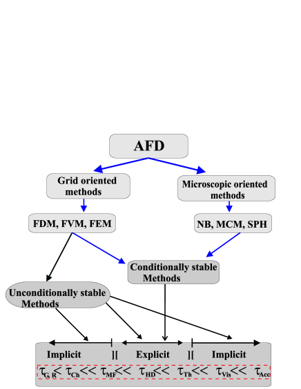
The numerical methods employed in AFD can be classified into two categories:

1. Microscopic oriented methods mostly based on N-body (NB), Monte-Carlo (MC) and on the Smoothed Particle Hydrodynamics (SPH).

2. Grid oriented methods. To this category belong the finite difference (FDM), finite volume (FVM) and finite-element methods (FEM).

Most numerical methods used in AFD are conditionally-stable. Hence, they may converge if the Courant-Friedlichs-Levy condition for stability is fulfilled. As long as efficiency is concerned, these methods are unrivalled candidates for flows that are strongly time-dependent and compressible. They may stagnate however, if important physical effects are to be considered or even if the flow is weakly incompressible. On the other hand, only a small number of the numerical methods employed in AFD are unconditionally stable. These are implicit methods, but they are effort-demanding from the programming point of view.
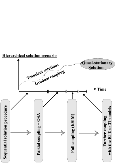
It has been shown that strongly implicit (henceforth IM) and explicit (henceforth EM) methods are different variants of the same algebraic problem (Hujeirat, 2005). Hence both methods can be unified within the context of the hierarchical solution scenario (henceforth HSS, see Fig. 3).

In Table 1 we have summarized the relevant properties of several numerical methods available.

	Explicit	Implicit	HSS
solution method	$q^{n+1}=q^{n}+\delta t\,d^{n}$	$q^{n+1}=q^{n}+\delta t\tilde{A}^{-1}d^{*}$	$q^{n+1}=\alpha q^{n}+(1-\alpha)\delta t\tilde{A}_{d}^{-1}d^{*}$
Type of flows	Strongly time- dependent, compressible, weakly dissipative HD and MHD in 1, 2 and 3 dimensions	Stationary, quasi-stationary, highly dissipative, radiative and axi-symmetric MHD-flows in 1, 2 and 3 dimensions	Stationary, quasi-stationary, weakly compressible, highly dissipative, radiative and axi-symmetric MHD-flows in 1, 2 and 3 dimensions
Stability	conditioned	unconditioned	unconditioned
Efficiency	$1$ (normalized/2D)	$\sim m^{2}$	$\sim m_{d}^{2}$
Efficiency: Enhancement strategies	Parallelization	Parallelization, preconditioning, multigrid	HSS, parallelization, preconditioning, prolongation
Robustness: Enhancement strategies	i. subtime-stepping ii. stiff terms are solved semi-implicitly	i. multiple iteration ii. reducing the time step size	i. multiple iteration ii. reducing the time step size, HSS
Numerical Codes Newtonian	Solvers1a ZEUS&ATHENAb, FLASHc, NIRVANAd, PLUTOe, VACf	Solver2g	IRMHDh
Numerical Codes Relativistic	Solvers3i GRMHDj, ENZOk, PLUTOl, HARMm, RAISHINn, RAMo, GENESISp, WHISKYq	Solver4r	GR-I-RMHDs

Table 1: A list of only a part of the grid-oriented codes in AFD and their algorithmic properties. In these equations, $q^{n,n+1}$, ${\delta t}$, ${\tilde{A}}$, $\alpha$ and $d^{*}$ denote the vector of variables from the old and new time levels, time step size, a preconditioning matrix, a switch on/off parameter and a time-modified defect vector, respectively. “m” in row 4 denotes the bandwidth of the corresponding matrix.

  ^aBodenheimer et al. (1978); Clarke (1996), ^bStone, Norman (1992); Gardiner, Stone (2006), ^cFryxell et al. (2000), ^dZiegler (1998), ^eMignone, Bodo (2003); Mignone et al. (2007), ^fTóth et al. (1998), ^gWuchterl (1990); Swesty (1995), ^hHujeirat (1995, 2005); Falle (2003), ⁱKoide et al. (1999); Komissarov (2004), ^jDe Villiers, Hawley (2003), ^kO’Shea et al. (2004), ^lMignone et al. (2007), ^mGammie et al. (2003), ⁿMizuno et al. (2006), ^oZhang, MacFadyen (2006), ^pAlay et al. (1999), ^qBaiotti et al. (2003), ^rLiebendörfer et al. (2002), ^sHujeirat et al. (2007).

Figure 1: Numerical methods (finite difference, finite volume, finite element, N-Body, Monte Carlo and the smoothed particle hydrodynamics employed in AFD and their possible regime of application from the time scale point of view. The time scales read as follows: the $\textrm{radiative-}\tau_{\mathrm{R}},~{}$ $\textrm{gravitative-}\tau_{\mathrm{G}},~{}$ $\textrm{chemical-}\tau_{\mathrm{Ch}},~{}$ $\textrm{magnetic-}\tau_{\mathrm{MF}},~{}$ $\textrm{hydrodynamic-}\tau_{\mathrm{HD}},~{}$ $\textrm{thermal-}\tau_{\mathrm{Th}},~{}$ $\textrm{viscous-}\tau_{\mathrm{Vis}},~{}$ and the $\textrm{accretion time scale-}\tau_{\mathrm{Acc}}.~{}$

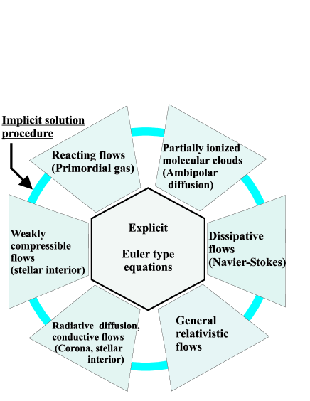
2 Time scales in AFD

Assume we are given a box of $L\times L\times L$ dimensions filled with a rotating multi-component gaseous-matter. The gas is said to be radiating, magnetized, chemical-reacting, partially ionized and under the influence of its own/external gravitational field. Let the initial state of the gas be characterized by a constant velocity, density, temperature and a constant magnetic field. The time-scales associated with the flow can be obtained directly from the radiative MHD-equations as follows (see Hujeirat, 2005, for detailed description of the set of equations).

Figure 2: The regime of application of explicit method is severely limited to Euler-type flows, whereas sophisticated treatment of most flow-problems in AFD require the employment of much more robust methods.

Scaling	variables	Molecular cloud	Accretion(onto SMBH)	Accretion (onto UCO)
$\tilde{L}$	Length	$\mathcal{O}(pc)$	$\mathcal{O}(\mathrm{AU})$	$\mathcal{O}(10^{6,}~{}\mathrm{cm})$
$\tilde{\rho}$	Density	$10^{-22}~{}\mathrm{g~{}cm}^{-3}$	$10^{-6}~{}\mathrm{g~{}cm}^{-3}$	$10^{-8}\rm{~{}g~{}cm^{-3}}$
$\tilde{\mathcal{T}}$	Temperature	10 K	$10^{6}$ K	$10^{7}$ K
$\tilde{V}$	Velocity	$0.3~{}\rm{km~{}s}^{-1}$	$10^{2}~{}\rm{km~{}s}^{-1}$	$10^{2-3}~{}\rm{km~{}s}^{-1}$
$\tilde{B}$	Magnetic Fields	$30~{}\mu$ G	$10^{2}~{}\mathrm{G}$	$10^{4}~{}\mathrm{G}$
$\tilde{\mathcal{M}}$	Mass	$10^{3}~{}\mathrm{M}_{\odot}$	$10^{6}~{}\mathrm{M}_{\odot}$	$~{}\mathrm{M}_{\odot}$
$\tilde{\rule[0.0pt]{0.0pt}{8.61108pt}}\,\dot{\cal M}$	Accretion rate		$10^{-2}~{}\mathrm{M}_{\odot}~{}\mathrm{Y}^{-1}$	$10^{-10}~{}\mathrm{M}_{\odot}~{}\mathrm{Y}^{-1}$

Table 2: A list of possible scaling variables typical for three different astrophysical phenomena: giant molecular clouds, accretion onto supermassive black holes (SMBHs) and accretion onto ultra-compact objects (UCO). These variables may be used for reformulating the radiative MHD equations in non-dimensional form.

• Continuity equation:

  $$\frac{\partial\rho}{\partial t}+\nabla\cdot\rho V=0,$$ (1)

  where $\rho,V$ stand for the density and the velocity field. Using scaling variables (e.g. Table 2), we may approximate the terms of this equation as follows:

  $$\frac{\partial\rho}{\partial t}\sim\frac{{\rho}}{\tau}~{}~{}\textrm{ and}~{}~{}\nabla\cdot\rho V\sim\frac{{\rho}~{}{V}}{{L}}.\\ \textrm{ This yields the hydrodynamical time scale}~{}~{}\tau_{HD}=\frac{{L}}{{V}}.\\$$

  The so-called accretion time scale can be obtained by integrating the continuity equation over the whole fluid volume. Specifically,

  $$\int_{Vol}{\frac{\partial\rho}{\partial t}}\,dVol=\frac{\partial M}{\partial t}\sim\frac{{M}}{\tau},~{}~{}~{}~{}~{}~{}~{}~{}~{}~{}\int_{Vol}{(\nabla\cdot\rho V)}\,dVol=\int_{S}\rho V\cdot n\cdot dS=\Delta\dot{M}\sim\dot{M},\\$$

  where “Vol” denotes the total volume of the gas and “S” corresponds to its surface. Equating the latter two terms, we obtain:

  $$\frac{M}{\tau}\sim\dot{M}\Rightarrow\tau_{acc}\sim\frac{M}{\dot{M}}.$$

  In general $\tau_{acc}$ is one of the longest time scales characterizing astrophysical flows connected to the accretion phenomena.

• The momentum equations:

  $$\frac{\partial V}{\partial t}+\nabla V\otimes V=-\frac{1}{\rho}\nabla P+f_{cent}+\frac{f_{\mathrm{rad}}}{\rho}+\nabla\psi+\frac{\nabla\times B\times B}{4\pi\rho}+Q^{\mathrm{r}}_{\mathrm{vis}},$$ (2)

  where $P,~{}f_{cent},~{}f_{\mathrm{rad}},~{}\psi,~{}B,~{}Q^{\mathrm{r}}_{\mathrm{vis}}$ denote gas pressure, centrifugal force, radiative force, gravitational potential, magnetic field and viscous operators, respectively. From this equation, we may obtain the following time scales:

  1. The sound speed crossing time can be obtained by comparing the following two terms:

     $$\frac{\partial V}{\partial t}\approx\frac{\nabla P}{\rho},~{}~{}~{}~{}\textrm{~{}~{}~{}~{}which yields:}~{}~{}~{}~{}\tau_{s}\approx\tau_{HD}~{}\left(\frac{V}{V_{s}}\right)^{2},$$

     where $V_{s}$is the sound speed.

  2. The gravitational time scale:

     $$\frac{\partial V}{\partial t}\approx\nabla\psi\Rightarrow\tau_{G}=~{}\tau_{HD}~{}\left(\frac{V}{V_{g}}\right)^{2},$$

     where $V^{2}_{g}=GM/L$ and G is the gravitational constant.

  3. Similarly, the Alf$\grave{\rm v}$en-wave crossing-time:

     $$\frac{\partial V}{\partial t}\approx\frac{\nabla\times B\times B}{4\pi\rho}\Rightarrow\tau_{mag}=~{}\tau_{HD}~{}\left(\frac{V}{V_{A}}\right)^{2},$$

     where $V^{2}_{A}(=B^{2}/4\pi\rho)$ denotes the Alf$\grave{\rm v}$en speed squared.

  4. Radiative effects in moving flows propagate on the radiative scale, which is obtained from:

     $$\frac{\partial V}{\partial t}\approx\frac{f_{\mathrm{rad}}}{\rho}\Rightarrow\tau_{rad}=~{}\tau_{HD}~{}\left(\frac{V}{c}\right)^{2},$$

     where c is the speed of light.

  5. The viscous time scale:

     $$\frac{\partial V}{\partial t}\approx Q^{\mathrm{r}}_{\mathrm{vis}}\sim\frac{\nu V}{L^{2}}\Rightarrow\tau_{vis}=\frac{L^{2}}{\nu}$$

     where $\nu$ is a viscosity coefficient.

• The induction equation, taking into account the effects of $\alpha_{\mathrm{dyn}}-$dynamo, magnetic diffusivity $\nu_{\mathrm{diff}}$ and of ambipolar diffusion reads:

  $$\frac{\partial B}{\partial t}=\nabla\times\langle V\times B+\alpha_{\mathrm{dyn}}B-\nu_{\mathrm{mag}}\nabla\times B\rangle+\nabla\times\{\frac{B}{4\pi\gamma\rho_{i}\rho_{n}}\times[B\times(\nabla\times B)]\},$$ (3)

  where $\rho_{\mathrm{i,n}}$ denote the ion and neutral densities.
  

  Thus, the induction equation contains several important time scales:

  1. The dynamo amplification time scale, which results from the equality:

     $$\frac{\partial B}{\partial t}=\nabla\times\alpha_{\mathrm{dyn}}B\Rightarrow\tau_{dyn}=\frac{L}{\alpha_{\mathrm{dyn}}}$$

  2. The magnetic-diffusion time scale:

     $$\frac{\partial B}{\partial t}=\nabla\times(\nu_{\mathrm{mag}}\nabla\times B)\Rightarrow\tau_{diff}=\frac{L^{2}}{\nu_{mag}}$$

  3. The ambipolar diffusion time scale:

     $$\frac{\partial B}{\partial t}=\nabla\times\{\frac{B}{4\pi\gamma\rho_{i}\rho_{n}}\times[B\times(\nabla\times B)]\}$$

     $$\Leftrightarrow\frac{B}{\tau}\sim\frac{1}{L}\left(\frac{B^{2}}{4\pi\rho_{n}}\right)\left(\frac{1}{\gamma\rho_{i}}\right)\left(\frac{B}{L}\right)\sim\frac{V^{2}_{A}}{\gamma\rho_{i}}\frac{B}{L^{2}}=\mathcal{D}_{amb}\frac{B}{L^{2}}\Rightarrow\tau_{amb}=\frac{L^{2}}{\mathcal{D}_{amb}},$$

     where $\mathcal{D}_{amb}(=V^{2}_{A}/(\gamma\rho_{i}))$ is the ambipolar diffusion coefficient.

• The chemical reaction equations.
  The equation describing the chemical-evolution of species $``i"$ is :

  $$\frac{\partial\rho_{i}}{\partial t}=\sum_{m}\sum_{n}k_{mn}{\rho_{m}}{\rho_{n}}+\sum_{m}I_{m}{\rho_{m}},$$ (4)

  where $k_{mn}$ denotes the reaction rate between the species ${m}$ and ${n}.$ $I_{m}$ stands for other external sources. For example, the reaction equation of atomic hydrogen in a primordial gas reads:

  $$\frac{\partial\rho_{H}}{\partial t}=\frac{k_{2}}{m_{H}}\rho_{H^{+}}\rho_{e}-\frac{k_{1}}{m_{H}}\rho_{H}\rho_{e}\Leftrightarrow\frac{\rho_{H}}{\tau}\sim\frac{k_{2}}{m_{H}}~{}\rho_{H}~{}\rho_{e}\Rightarrow\tau_{ch}\sim\frac{m_{H}}{k_{2}~{}\rho_{e}},$$

  where $\rho_{e},~{}k_{2}(10^{-10}~{}\rm cm^{3}~{}s^{-1})$ correspond to the electron density and to the generation rate of atomic hydrogen through the capture of electrons by ionized atomic hydrogen. $~{}m_{H}$ corresponds to the mass of atomic hydrogen.

• Equations of relativistic MHD

  The velocities in relativistic flows are comparable to the speed of light. This implies that the hydrodynamical $\tau_{HD}$ and radiative $\tau_{rad}$ time scales are comparable and that both are much shorter than in Newtonian flows.

Time scales	Molecular cloud	Accretion(onto SMBH)	Accretion (onto UCO)
$\tau_{HD}$	$\sim 10^{6}\rm{~{}Yr}$	$\sim$ months	$\sim 1$ s
$\tau_{rad}/\tau_{HD}$	$\sim 10^{-6}$	$\sim 10^{-3}$	$\sim 10^{-3}$
$\tau_{grav}/\tau_{HD}$	$\sim 10^{-2}$	$\sim 10^{-3}$	$\sim 10^{-3}$
$\tau_{ch}/\tau_{HD}$	$\sim 10^{-1}$	$\sim 10^{-5}$	$\sim 10^{-4}$
$\tau_{mag}/\tau_{HD}$	$\sim 10^{-2}$	$\sim 10^{0}$	$\sim 10^{-1}$
$\tau_{vis}/\tau_{HD}$	$\sim 10^{1}$	$\sim 10^{2}$	$\sim 10^{2}$
$\tau_{acc}/\tau_{HD}$		$\sim 10^{4}$	$\sim 10^{12}$

Table 3: A list of the time scales relative to the hydrodynamical time scale for three different astrophysical phenomena.

We note that although the dynamical time scale in relativistically moving flows is relatively short, there are still several reasons that justify the use of implicit numerical procedures. In particular:

1. The relativistic MHD equations are strongly non-linear, giving rise to fast growing non-linear perturbations, imposing thereby a further restriction on the size of the time step.

2. The deformation of the geometry grows non-linearly when approaching the black hole. Thus, in order to capture flow-configurations in the vicinity of a black hole accurately, a non-linear distribution of the grid points is necessary, which, again, may destabilize explicit schemes.

3. Initially non-relativistic flows may become ultra-relativistic or vice versa. However, almost all non-relativistic astrophysical flows known to date are considered to be dissipative and diffusive. Therefore, in order to track their time-evolution reliably, the employed numerical solver should be capable of treating the corresponding second order viscous terms properly.

4. The accumulated round off errors resulting from performing a large number of time-extrapolations for time-advancing a numerical hydrodynamical solution may easily cause divergence. The constraining effects of boundary conditions may fail to configure the final numerical solution.

Figure 3: A schematic description of the hierarchical solution scenario (HSS). The HSS is based on dynamical-varying the efficiency and robustness of the numerical method to leapfrog the transient phase. The method is most suitable for searching quasi-stationary flow-configurations that depend weakly on the initial conditions. Here the coupling between the equations can be enhanced gradually, by starting solving them sequentially, then partial-coupling in combination with the operator splitting approach (OSA), full-coupling using the Krylov-subspace iterative method (KSIM) and finally extending the coupling to include the radiative transfer equation (RTE) and energy equation of multi-temperature plasmas.

3 Numerical methods: a unification approach

In this section we show that explicit and implicit methods are special cases of a more general solution method in higher dimensions.
Assume we are given the following evolution equation of a vector variable $q$:

$$\frac{\partial q}{\partial t}+L(q)=f,$$ (5)

where $L,f$ correspond to an advection operator and to external forces.

Adopting a time-forward discretization procedure, the unknown vector $q$ at the new time level can be extrapolated as follows:

$$q^{n+1}=q^{n}+\delta t\cdot RHS^{n},$$ (6)

where $RHS=f-L(q).$

Depending on the time step size and on the number of grid points, the numerical procedure can be made sufficiently accurate in space and time.
On the other hand Equation 6 can be viewed as an equality of two one-dimensional vectors:

$$\textrm{[vector of unknowns] = [vector of knowns] }\Leftrightarrow~{}~{}~{}~{}~{}~{}q^{n+1}=\bar{b},$$ (7)

where $\bar{b}=q^{n}+\delta t\cdot RHS^{n}.$
In higher dimensions, however, Equation 7 is a special case of the matrix equation:

$$Aq^{n+1}=\bar{b},$$ (8)

in which it is projected along the diagonal elements. It is obvious that the matrix ${I/\delta t}$ is a further simplification of the matrix that contains just the diagonal elements of A.

Therefore, we may adopt the higher dimension formulation to gain a better understanding of the stability of the solution procedure.

Figure 4: The the profile of the shock tube problem obtained with Courant-Friedrichs-Levy numbers CFL=0.4 and 0.9 using the PLUTO code. Although both CFL-numbers are smaller than unity the numerical solution procedure does not appear to be stable even with CFL=0.9.

According to matrix algebra, a necessary condition for the matrix A to have a stable inversion procedure is that A must be strictly diagonally dominant. Equivalently, the entries in each row of the matrix A must fulfill the following condition: the module of the diagonal element $d_{i,i}$ is larger than the sum of all off-diagonal elements $\sum_{\mathrm{j\neq i}}{|a_{i,j}|},$ where i and j denote the row and column numbers of the matrix . Applying a conservative and monotonicity preserving scheme, the latter inequality may be re-written in the following form:

$$\left|\frac{1}{\delta t}+\textrm{positive contributions}\right|>\sum_{\mathrm{j(\neq i)}}{|a_{i,j}|}.$$ (9)

We note that since $\delta t$ is a free parameter, it can be chosen sufficiently small, so that $1/\delta t$ largely dominates all other off-diagonal elements, or so large that $1/\delta t$ becomes negligibly small.

We may further simplify this inequality by choosing the time step size even smaller, such that

$$\frac{1}{\delta t}>\sum_{j}|a_{i,j}|,~{}~{}~{}~{}~{}\textrm{for $\forall~{}~{}j\neq i$}$$ (10)

can be safely fulfilled. We may decompose the matrix A as follows:

$$A=D+R=D(I+D^{-1}R),$$

where D is the matrix consisting of the diagonal entries of A and $R~{}(=A-D)$ consists of the off-diagonals. Thus, the elements of D are proportional to $1/\delta t$, whereas those of R are proportional to $\delta t$. This implies that A can be expanded around $I/\delta t$ in the form:

$$A=A^{(0)}+A^{(1)}+A^{(2)}+\cdot\cdot\cdot,$$ (11)

where the leading matrix $A^{(0)}\approx\frac{1}{\delta\rm t}~{}\rm I~{}$ and $A^{(1)}\sim\delta\rm t~{}I.$ In this case the inversion of the matrix A is not more necessary and the resulting numerical procedure would correspond to a classical time-explicit method.

1 Example

The time-evolution of density in one-dimension is described by the continuity equation:

$$L_{\rho}=\frac{\partial\rho}{\partial t}+\frac{\partial\rho U}{\partial x}=0.$$ (12)

The corresponding Jacobian matrix is: $A=\partial{L_{\rho}}/{\partial\rho}.$ The non-zero entries of A read:

$$a_{ii}=\frac{1}{\delta t}+\frac{|U_{i}|}{\Delta x}\textrm{~{}~{}~{}~{}~{}and the off diagonal~{}~{}~{}}a_{ij}=-\frac{|U_{j+1}|}{\Delta x}\textrm{~{}~{}~{}~{}for i$\neq$ j~{}~{}~{}~{}, }$$ (13)

where ${\Delta x}$ and $i,j$ denote the grid spacing and grid point numbering. Applying a first order upwind discretization, then the condition of diagonal dominance demands:

$$\left|\frac{1}{\delta t}+\frac{U_{i}}{\Delta x}\right|>\frac{|U_{j+1}|}{\Delta x}.$$ (14)

This condition can be further simplified by choosing the time step size so small, such that

$$\frac{1}{\delta t}>\frac{2~{}\max\,(|U_{j}|,|U_{j+1}|)}{\Delta x}\Leftrightarrow\frac{{\delta t}\,\max\,(|U_{j}|,|U_{j+1}|)}{\Delta x}<\frac{1}{2}.$$ (15)

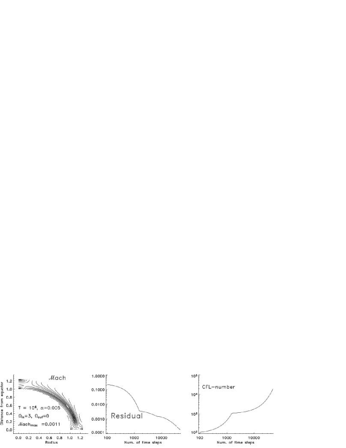
Thus, the condition of diagonal dominance is more restrictive than the normal CFL condition. This may explain, why most explicit methods fail to converge for Courant-Friedrichs-Levy number CFL $=1-\epsilon~{}~{}~{}$ (see Fig. 4).

Figure 5: Weakly incompressible flow between two concentric rotating spheres. Left panel: the 2D-distribution of $\textrm{Mach number (= V/V}_{\mathrm{s}})~{}~{}$ is displayed (25 isolines) for extreme weakly incompressible flows $(Max~{}(Mach)\sim~{}10^{-3}).$ The maximum residual (middle) and the CFL-number (right) versus the number of time steps are shown.

4 Converting time-explicit into implicit solution methods

In a series of publications, we have shown that the robustness of explicit methods can be enhanced gradually to recover full-implicit solution procedures (see Hujeirat, 2005). In the following we outline the main algorithmic steps towards extending classical explicit methods into implicit:

1. Use the same mathematical form of $RHS^{n}$ of Eq. 6 to compute $RHS^{n+1}=RHS(q^{n+1})$ and subsequently the mean $\overline{RHS}=\alpha\cdot{RHS^{n}}+(1-\alpha)\cdot RHS^{n+1},$ where $0\leq\alpha\leq 1$ is a parameter that may depend also on the time step size.

2. Define the defect

   $$d=-(\frac{q^{n+1}-q^{n}}{\delta t})+\overline{RHS}.$$ (16)

3. Compute the Jacobian $J^{real}=\partial L_{q}/\partial q$, where $L_{q}$ denotes the set of equations in operator form.

4. Construct a simplified matrix $\tilde{A}$ (preconditioner), which is easy to invert, but still share the spectral properties of $J^{real}$ (Hackbusch, 1994).

   

   

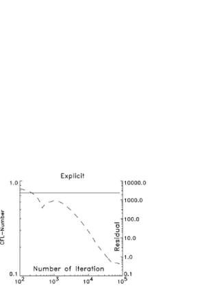
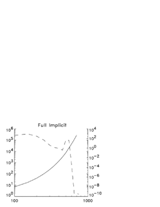
   Figure 6: The profiles of the CFL-number (solid line) versus the number of iteration both for explicit and implicit solution procedures (dashed line). The profiles correspond to the free-fall of spherical plasma onto a non-magnetized Schwarzschild black hole, in which the final solution is time-independent.

5. Solve the system of equation:

   $$\tilde{A}\mu=d,$$ (17)

   where $\mu$ is a vector of small correction, so that $q^{l+1}=q^{l}+\mu.$
   In general $\tilde{A}\neq J^{real},$ which implies that Equation 17 should be solved iteratively to assure that the maximum norm of the defect, $||d||_{\infty},$ is sufficiently small.

We note that for sufficiently small $\delta t$, the matrix $I/\delta t$ can be made similar to $J^{real}$, hence they share the same spectral space. As a consequence, a variety of solution procedures can be constructed that range from purely explicit up to strongly implicit, depending on how similar the preconditioner $\tilde{A}$ is to the real Jacobian. This naturally suggests the hierarchical solution scenario as a highly powerful numerical algorithm for enhancing the robustness of explicit schemes and optimizing their efficiency (Fig. 3, see also Hujeirat, 2005)

5 Summary-I

In this part of the review we have presented a method for converting conditionally-stable explicit methods into numerically stable implicit solution procedures. The conversion method allows a considerable enlargement of the range of application of explicit methods. The hierarchical solution scenario is best suited for gradual enhancement of their robustness and optimizing their efficiency.

Part II

(Magneto-)Hydrodynamic Boltzmann Solvers

In this part, I will discuss the implementation of a time-explicit gas-kinetic grid-based integrator for non-relativistic hydrodynamics introduced by Prendergast & Xu (1993), Xu (1999) and Tang & Xu (2000), and its extension to non-ideal magneto-hydrodynamics (Heitsch et al. 2004, 2007). Some properties of Boltzmann solvers are discussed in §6, the equations and the implementation are described in §7, followed by a selection of test cases and applications (§8) and a summary (§9).

6 Why Boltzmann Solvers?

It is the physical model for the fluid equations which distinguishes gas-kinetic schemes from the widely popular Godunov methods. The latter are formulated on the basis of the Vlasov-equation, i.e. assuming that any dynamical time scale is larger than the collision time between particles, setting the collision term in the Boltzmann equation to zero. The distribution function is then given by a Maxwellian at all times. In contrast, gas-kinetic schemes keep the collision term in the Boltzmann equation, but because of the impractibility to compute all the collisions between particles, they need to come up with a model for the collision term.

One such model has been introduced by Bhatnagar, Gross & Krook (1954), formulating the collision term as the difference between the equilibrium distribution function $g$ (the Maxwellian) and the initial distribution function $f$, resulting in a Boltzmann equation of the form

$$\partial_{t}f+u\partial_{x}f+\dot{u}\partial_{u}f=\frac{g-f}{\tau},$$ (18)

where $\tau$ is the collision time. Integrating eq. 18 over a time $t$ gives (at position $x$)

$$f(x,t,u)=\frac{1}{\tau}\int_{0}^{t}g(x-u(t-t^{\prime}),t^{\prime},u)\,e^{-(t-t^{\prime})/\tau}dt^{\prime}+e^{-t/\tau}\,f_{0}(x-ut,0,u),$$ (19)

where $\tau$ is the collision time, and $f_{0}$ the initial distribution function. For a complete description, see Xu (2001). Thus, the distribution function $f$ at time $t$ gets two contributions: one from the decaying initial conditions $f(t=0)$, and one from the growing equilibrium distribution $g$.

The 0th, 1st and 2nd order velocity moments of the distribution function (here for a monatomic gas)

$$g\equiv\rho\left(\frac{\lambda}{\pi}\right)^{3/2}\,\exp(\lambda(\mathbf{u}-\mathbf{U})^{2})$$ (20)

result in the (macroscopic) conserved quantities density $\rho$, momentum density $\rho U$ and total energy density $\rho E$. The quantity $\lambda\equiv m/(2kT)$. The corresponding moments of the Boltzmann equation 18 give the conservation equations. The BGK collision term in eq. 18 gives then rise to a viscous flux, depending on the ratio of the CFL time step and a specified collision time. Thus, the Reynolds number of the flow can be controlled. The Prandtl number is 1 by construction. The scheme is upwind and it satisfies the entropy condition (Prendergast & Xu 1993, Xu 2001). The fully controlled dissipative term come at (close) to no extra computational cost. Fragmentation of hydrodynamically unstable systems due to numerical noise thus can be suppressed. Specifically, gas-kinetic schemes can easily provide a viscosity independent of grid geometry, thus allowing e.g. the modeling of disks on a cartesian grid (see Slyz et al. 2002).

In the following I will discuss a specific implementation of a gas-kinetic solver, namely Proteus (see Heitsch et al. 2007).

7 Equations and Implementation: Proteus

Proteus solves the equations of non-ideal magnetohydrodynamics, with an Ohmic resistivity $\lambda_{\Omega}$, and a shear viscosity $\nu$.

$$\partial_{t}\rho+\mathbf{\nabla}\cdot(\rho\mathbf{v})=0$$ (21)

$$\partial_{t}\rho\mathbf{v}+\mathbf{\nabla}\cdot\left[\rho\mathbf{v}\mathbf{v}-\frac{\mathbf{B}\mathbf{B}}{4\pi}+p+\frac{\mathbf{B}^{2}}{8\pi}\right]=\mathbf{\nabla}\cdot\bar{{\bf\Pi}}$$ (22)

$$\partial_{t}\rho E+\mathbf{\nabla}\cdot\left[\rho E\mathbf{v}+(p+\frac{\mathbf{B}^{2}}{8\pi})\mathbf{v}-\frac{(\mathbf{v}\cdot\mathbf{B})\mathbf{B}}{4\pi}\right]=\mathbf{v}\cdot\left(\mathbf{\nabla}\cdot\bar{{\bf\Pi}}\right)+\lambda_{\Omega}\mathbf{J}^{2}$$ (23)

$$\partial_{t}\mathbf{B}+\mathbf{\nabla}\cdot(\mathbf{v}\mathbf{B}-\mathbf{B}\mathbf{v})=\lambda_{\Omega}\mathbf{\nabla}^{2}\mathbf{B},$$ (24)

The mechanism how to split the fluxes at the cell walls is described in detail by Xu (1999) and will not be repeated here. Viscosity and resistivity are implemented as dissipative fluxes. They require spatially constant coefficients $\lambda_{\Omega}$ and $\nu$. Ambipolar drift is implemented in the two-fluid description, currently only for an isothermal equation of state, though.

Higher-order time accuracy is achieved by a TVD Runge-Kutta time stepping (Shu & Osher 1988). For second-order spatial accuracy, a choice of reconstruction prescriptions is available.

Proteus offers two gas-kinetic solvers, the one just described, and a one-step integrator at 2nd order in time and space for hydrodynamics. The latter has been discussed in detail by Slyz & Prendergast (1999) and Slyz et al. (2005), so that we refer the interested reader to those papers.

8 Test Cases and Applications

1 1D: Resistively damped Linear Alfven Wave

This one-dimensional test checks the resistive flux implementation as well as the accuracy of teh overall scheme. A linear Alfén wave under weak Ohmic dissipation is damped at a rate of

$$\omega_{i}=\frac{1}{2}\lambda_{\Omega}k^{2}$$ (25)

where $\lambda_{\Omega}$ is the Ohmic resistivity, and $k=2\pi\kappa/L$ is the wave number of the Alfvén wave, with $\kappa$ a natural number. The strongly damped case, where the decay dominates the time evolution, is uninteresting for our application, since the Ohmic resistivity is mainly used to control numerical dissipation. Figure 7 shows the damping rate against Ohmic resistivity $\lambda_{\Omega}$ for $\kappa=1,2,4$ at a grid resolution of $N=64$. The damping rate is derived by measuring the amplitude of the wave at each full wave period.

Figure 7: Logarithm of the damping rate (eq. [25]) of a linear Alfvén wave against logarithm of the Ohmic resistivity for $\kappa=1,2,4$. The resolution is $N=64$. Lines denote the analytical solution.

From Figure 7, it is clear that, as one diminishes the value of $\lambda_{\Omega}$, there comes a point when the numerical resistivity of the scheme becomes comparable to the physical one, causing the measured damping rate to flatten out and depart from the analytical solution. For $\kappa=4$ and $\lambda_{\Omega}=0.1$, the wave decays too quickly to allow a reliable measurement, and the system enters the strongly damped branch of the dispersion relation. However, we emphasize that even at $16$ cells per wave length the resistivity range available to Proteus spans nearly two orders of magnitude.

2 1D: Linear Alfven Waves in Weakly Ionized Plasmas

The dispersion relation for a linear Alfvén wave in a weakly ionized plasma splits into two branches (Kulsrud & Pearce 1969): a strongly coupled branch, for which the ion Alfvén frequency $\omega_{k}\equiv kB/\sqrt{4\pi\rho_{i}}\ll\nu_{in}\equiv\gamma\rho_{n}$, the ion-neutral collision frequency, and a weakly coupled branch, for which $\omega_{k}\gg\nu_{in}\sqrt{\rho_{i}/\rho_{n}}$. The strongly coupled case leads to a dispersion relation of

$$\omega=\pm\left(\omega_{k}^{2}\epsilon-\frac{\omega_{k}^{4}}{4\nu_{in}}\right)^{1/2}-\imath\frac{\omega_{k}^{2}}{2\nu_{in}},$$ (26)

with $\epsilon\equiv\rho_{i}/rho_{n}$. Thus, the strongly coupled Alfvén wave travels at the neutral Alfvén speed $c_{An}\equiv B/\sqrt{4\pi\rho_{n}}$ and is increasingly damped with decreasing collision frequency. The weakly coupled branch leads to

$$\omega=\pm\left(\omega_{k}^{2}-\frac{\nu_{in}^{2}}{4}\right)^{1/2}-\imath\frac{\nu_{in}}{2}.$$ (27)

Now, the wave travels at the ion Alfvén speed, and damping is proportional to $\nu_{in}$. Since $c_{An}\sqrt{\rho_{n}/\rho_{i}}$, the speeds can be widely disparate.

Figure 8: Logarithm of the frequency (upper panel) and damping rate (lower panel) for the linear Alfvén wave in a partially ionized plasma. For simplicity, we vary the collision coefficient $\gamma_{AD}$ instead of the density.

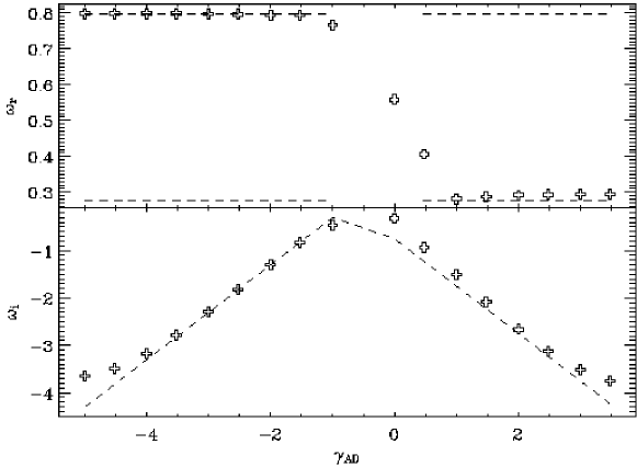
Figure 8 shows the real and imaginary part of the Alfvén wave frequency in a weakly ionized plasma. For simplicity, we vary the collision coefficient $\gamma_{AD}$ and keep the densities constant. Wave speed (upper panel) and damping term (lower panel) are well reproduced.

3 2D: Current Sheet

This test is taken from Gardiner & Stone (2005). A square domain of extent $0\leq x,y\leq 2$ and of constant density $\rho_{0}=1$ and pressure $p_{0}=0.1$ is permeated by a magnetic field along the $y$ direction such that $B_{y}(0.5<x<1.5)=-1$, and $B_{y}=1$ elsewhere. The ratio of thermal over magnetic pressure is $\beta=0.2$. This setup results in two magnetic null lines, which then are perturbed by velocities $v_{x}=v_{0}\sin(\pi y)$. Here, we use an adiabatic exponent of $\gamma=5/3$ and employ the conservative formulation of the scheme. Figure 9 summarizes the test results in the form of the magnetic energy density $\langle B^{2}\rangle$ against time. Different line styles stand for resistivities, and the line thickness denotes the model resolution. We ran tests at $N=128^{2}$, $256^{2}$ and $512^{2}$. All models ran up to $t=4$ and farther except for the $512^{2}$-model at $\lambda_{\Omega}=0$. A finite resistivity helps stabilizing the code.

Figure 9: Current sheet test. Magnetic energy density $\langle B^{2}\rangle$ against time. A finite resistivity $\lambda_{\Omega}$ helps stabilize the code. Line thickness stands for resolution, line style for resistivity.

The evolution of the system follows that described by Gardiner & Stone (2005), including the merging of magnetic islands until there are two islands per magnetic null line left, located approximately at the velocity anti-nodes. For zero resistivity (solid lines), the magnetic energy decay depends strongly on the resolution. This effect is reduced by increasing $\lambda_{\Omega}$. For $\log\lambda_{\Omega}=-5$ (dashed lines), the energy evolution follows pretty much the curves for $\lambda_{\Omega}=0$ (solid lines), indicating insufficient resolution. For $\log\lambda_{\Omega}=-4$, the two higher resolutions start to separate from the lower resolution run, while at $\log\lambda_{\Omega}=-3$, the two higher resolutions lead to indistinguishable curves (dash-3dot lines).

4 2D: Advection of a Field Loop

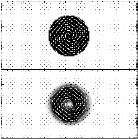
A cylindrical current distribution (i.e. a field loop) is advected diagonally across the simulation domain. Again, we follow the implementation presented by Gardiner & Stone (2005). Density and pressure are both initially uniform at $\rho_{0}=1$ and $p_{0}=1$, and the fluid is described as an ideal gas with an adiabatic exponent of $\gamma=5/3$. The computational grid at a resolution of $N_{x}\times N_{y}=128\times 64$ extends over $-1.0\leq x\leq 1.0$ and $-0.5\leq y\leq 0.5$. The field loop is initialized via the $z$-component of the vector potential $A_{z}=a_{0}(R-r)$, where $a_{0}=10^{-3}$, $R=0.3$ and $r\equiv(x^{2}+y^{2})^{1/2}$. The loop is advected at an angle of $30$ degrees with respect to the $x$-axis. Thus, two round trips in $x$ correspond to one crossing in $y$. Figure 10 shows the initial magnetic energy density $B^{2}$ with the magnetic field vectors over-plotted (top), and the $B^{2}$ distribution after two time-units measured in horizontal crossing times (bottom). The overall shape is preserved, although some artifacts are visible. These results concerning the shape are similar to those of Gardiner & Stone (2005), specifically, Proteus preserves the circular field lines. This test uses $\lambda_{\Omega}\equiv 0$.

Figure 10: Field loop advection test: magnetic energy density $B^{2}$ at $t=0$ (top) and at $t=2$ corresponding to two horizontal crossing times (bottom), with over-plotted field vectors. The grid resolution is $N_{x}\times N_{y}=128\times 64$.

The time evolution of the magnetic energy density corresponding to Figure 10 is shown in Figure 11. Diamonds stand for Proteus results, the energy decay observed by Gardiner & Stone (2005) with ATHENA is indicated by the solid line, following their analytical fit. The energies are normalized to 1. Clearly, Proteus is somewhat more diffusive.

Figure 11: Normalized magnetic energy density against time (in units of horizontal crossing time) with the same parameters as in Figure 10. Diamonds stand for Proteus results, and the energy evolution as observed in ATHENA is shown by the solid line.

In summary, these numerical test cases demonstrate that Proteus models dissipative MHD effects accurately. Furthermore, it can advect geometrically complex magnetic field patterns properly.

9 Summary

Gas-kinetic schemes provide a robust and physical mechanism to solve the equations of magneto-hydrodynamics. Dissipative effects can be fully controlled. I discussed a specific implementation of a gas-kinetic solver – Proteus –, including resistivity and (two-fluid) ambipolar diffusion. Details of the implementation have been presented elsewhere (Tang & Xu 2000, Heitsch et al. 2004, 2007), and an application to shear flows in magnetized fluids will be discussed by Palotti et al. (2008). 99

Aloy, M.-A., Ibanez, J.M., Mart, J.M., Müller, E., 1999, ApJS, 122, 151 (GENESIS)

Anninos, P., Fragile, P. C., 2003, ApJ. Suppl. Ser., 144, Iss. 2, 243-257

Baiotti, L., Hawke, I., Montero, P.J., Rezzolla, L., 2003, MSAIS, 1, 210

Bhatnagar, P. L., Gross, E. P. and Krook, M. (1954). A Model for Collision Processes in Gases. I. Small Amplitude Processes in Charged and Neutral One-Component Systems, Phys. Rev. 94, 511-525.

Bodenheimer, P., Tohline, J. E., Black, D. C., 1978, BAAS, 10, 655

Clarke, D.A., 1996, APJ, 457, 291

De Villiers, J.-P., Hawley, J.F., 2003, ApJ, 589, 458

Falle, S.A.E.G., 2003, astro-ph/0308396

Fryxell, B. et al., 2000, ApJS, 131, 273-334 (FLASH)

Gammie, C. F., McKinney, J. C., Tóth, G., 2003, ApJ, 589, 444-457 (HARM)

Gardiner, T. A. and Stone, J. M. (2005). An unsplit Godunov method of ideal MHD via constrained transport, J. of Comp. Phys. 205, 509-539.

Gardiner, T.A., Stone, J.M., 2006, ASPC, 359, 143

Hackbusch, W., 1994, “Iterative Solution of Large Sparse Systems of Equations”, Springer–Verlag, New York-Berlin-Heidelberg

Heitsch, F., Zweibel, E. G., Slyz, A. D., and Devriendt, J. E. G. (2004). Turbulent Ambipolar Diffusion: Numerical Studies in Two Dimensions, Astrophys. J. 603, 165-179

Heitsch, F., Slyz, A. D., Devriendt, J. E. G., Hartmann, L. W., and Burkert, A. (2007). Magnetized Nonlinear Thin-Shell Instability: Numerical Studies in Two Dimensions, Astrophys. J. 665, 445-456

Hujeirat, A., 1995, A&A,295, 268

Hujeirat, A., Rannacher, R., 2001, New Ast. Reviews, 45, 425

Hujeirat, A., 2005, CoPhC, 168, 1

Hujeirat, A., Camenzind 2007, Keil, B., arXiv, 0705.125

Kulsrud, R. and Pearce, W. P. (1969) The Effect of Wave-Particle Interactions on the Propagation of Cosmic Rays, Astrophys. J. 156, 445-469

Koide, S., Shibata K., Kudoh, T., 1999, ApJ, 522, 727

Komissarov, S.S., 2004, MNRAS, 350, 1431

Liebendörfer, M., Rosswog, S., Thielemann, F.-K., 2002, ApJS, 141, 229L

Mignone, A., Bodo, G., 2003, NewAR, 47, 581

Mignone, A., Bodo, G., Massaglia, S., Matsakos, T., Tesileanu, O., Zanni, C., Ferrari, A., 2007, ApJS, 170, 228-242 (PLUTO)

Mizuno, Y., Nishikawa, J.-I., et al., 2006, astro-ph/0609004 (RAISHIN)

O’Shea, B.W., Bryan, G., Bordner, J., Norman, M. L., Abel, T., Harkness, R., Kritsuk, A., 2004, astro-ph/0403044 (ENZO)

Palotti, M. L., Heitsch, F., Zweibel, E. G., and Huang, Y.-M. (2008). Evolution of Unmagnetized and Magnetized Shear Layers, Astrophys. J., submitted

Prendergast, K.-H. and Xu, K. (1993). Numerical Hydrodynamics from Gas-Kinetic Theory, J. Comp. Phys., 109, 53-66

Shu, C.-W. and Osher, S. (1988) Efficient Implementation of Essentially Non-oscillatory Shock-capturing Schemes. J. Comp. Phys. 77, 439-471

Slyz, A. D. and Prendergast, K. H. (1999). Time-independent gravitational fields in the BGK scheme for hydrodynamics, Astro. & Astrophys. Supp. 139, 199-217

Slyz, A. D., Devriendt, J. E. G., Bryan, G. and Silk, J. (2005). Towards simulating star formation in the interstellar medium, MNRAS 356, 737-752

Stetter, H.J., 1978, Numer. Math., 29, 425–443

Stone, J.M., Norman, M.L., 1992, ApJS, 80, 753

Swesty, F.D., 1995, ApJ, 445, 811

Tang, H.-Z. and Xu, K. (2000). A High-Order Gas-Kinetic Method for Multidimensional Ideal Magnetohydrodynamics, J. Comp. Phys. 165, 69-88

Tóth, G., Keppens, R., Botchev M.A., 1998, A&A, 332, 1159 (VAC)

Wuchterl, G., 1990, A&A, 238, 83

Xu, K. (1999) Gas-kinetic Theory-based Flux Splitting Method for Ideal Magnetohydrodynamics, J. Comp. Phys. 153, 334-352.

Xu. K. (2001) A Gas-kinetic BGK Scheme for the Navier-Stokes Equations and its Connection with Artificial Dissipation and Godunov Method (2001). J. Comp. Phys. 171, 289-335.

Zhang, W., MacFadyen, A. I., 2006, ApJS, 164, 255-279 (RAM)

Ziegler, U., 1998, Comp. Phys. Comm., 109, 111 (NIRVANA)