Phase-ordering kinetics of two-dimensional disordered Ising models

Abstract

The phase-ordering kinetics of the ferromagnetic $2D$ Ising model with uniform disorder is investigated by intensive Monte Carlo simulations. Taking into account finite-time corrections to scaling, simple ageing behaviour is observed in the two-time responses and correlators. The dynamical exponent $z$ and the form of the scaling functions only depend on the ratio $\varepsilon/T$, where $\varepsilon$ describes the width of the distribution of the disorder. The agreement of the predictions of local scale-invariance generalised to $z\neq 2$ for the two-time scaling functions of response and correlations with the numerical data provides a direct test of generalised Galilei-invariance.

1 Introduction

A ferromagnetic system quenched from an initially disordered state into its coexistence phase with at least two equivalent equilibrium states undergoes phase-ordering kinetics, driven by the surface tension between the ordered domains whose linear size grows as $L=L(t)\sim t^{1/z}$ where $z$ is the dynamical exponent. For a non-conserved order-parameter it is well-known that $z=2$, see [1] for a review. Phase-ordering is one of the instances where physical ageing occurs, by which we mean the following properties: (i) slow (i.e. non-exponential) dynamics, (ii) breaking of time-translation invariance, and (iii) dynamical scaling. Because of the simple algebraic scaling of the linear domain size $L(t)$, two-time correlation and response functions are expected to display the following simple scaling forms in the ageing regime (where the observation time $t$ and the waiting time $s$, that are both measured since the quench, satisfy $t,s\gg t_{\rm micro}$ and $t-s\gg t_{\rm micro}$):

$$C(t,s;\boldsymbol{r}) := \langle\phi(t,\boldsymbol{r})\phi(s,\boldsymbol{0})\rangle=s^{-b}f_{C}\left(\frac{t}{s},\frac{\boldsymbol{r}}{(t-s)^{1/z}}\right)~{},~{}~{}~{}~{}$$ (1)

$$R(t,s;\boldsymbol{r}) := \left.\frac{\delta\langle\phi(t,\boldsymbol{r})\rangle}{\delta h(s,\boldsymbol{0})}\right|_{h=0}=s^{-1-a}f_{R}\left(\frac{t}{s},\frac{\boldsymbol{r}}{(t-s)^{1/z}}\right)~{}.$$

Here $\phi(t,\boldsymbol{r})$ is the space-time-dependent order-parameter, whereas $h(s,\boldsymbol{r})$ is the conjugate magnetic field (spatial translation-invariance will be assumed throughout this paper) and $a$ and $b$ are ageing exponents. The scaling functions $f_{C,R}(y,\boldsymbol{0})\sim y^{-\lambda_{C,R}/z}$ for $y\to\infty$ which defines the autocorrelation exponent $\lambda_{C}$ and the autoresponse exponent $\lambda_{R}$. For phase-ordering kinetics, it is generally admitted that $b=0$ and simple scaling arguments show that $a=1/z$. For an initial high-temperature state and for pure ferromagnets, $\lambda_{C}=\lambda_{R}$ is independent of the known equilibrium exponents [1, 2, 3]. More detailed information is contained in the form of the scaling functions $f_{C,R}(y,\boldsymbol{u})$. Indeed, for the phase-ordering kinetics of pure ferromagnets where $z=2$, it has been shown that dynamical scaling can be extended to a local scale-invariance (LSI) which in particular implies co-variance of the linear responses under transformations $t\mapsto t/(\gamma t+\delta)$ in time. The other important ingredient is the Galilei-invariance of the deterministic part of the associated stochastic Langevin equation. Explicit predictions for the scaling functions $f_{C,R}$ follow and numerous tests have been performed in a large variety of models and different physical situations, see the recent reviews [4, 5, 6] and references therein.

Here, we shall present tests of LSI in cases where the dynamical exponent $z\neq 2$. The foundations of the theory were presented some time ago in [7] and have been reformulated recently [8]. Several tests of LSI were performed in systems described by linear Langevin equations in cases where either $z=4$ [10, 9] or else $0<z<2$ [11]. In this letter, we present the first test of LSI as reformulated in [8] with $z\neq 2$ in a model where the corresponding Langevin equation is non-linear.

We consider a two-dimensional ferromagnetic Ising model with quenched disorder. The nearest-neighbour hamiltonian is given by [13, 12]

$$\mathcal{H}=-\sum_{(i,j)}J_{ij}\sigma_{i}\sigma_{j},\quad\sigma_{i}=\pm 1~{}.$$ (2)

The random variables $J_{ij}$ are uniformly distributed over $[1-\varepsilon/2,1+\varepsilon/2]$ where $0\leq\varepsilon\leq 2$. The model has a second-order phase transition at a critical temperature $T_{c}(\varepsilon)>0$ between a paramagnetic and a (diluted) ferromagnetic state. Using heat-bath dynamics such that the order-parameter is non-conserved and starting from a fully disordered initial state, phase-ordering occurs where the dynamical exponent is given by

$$z=z(T,\epsilon)=2+\epsilon/T~{}.$$ (3)

This formula can be derived from phenomenological scaling arguments which assume that the disorder is creating defects with logarithmically distributed barrier heights parametrised by the constant $\epsilon$ [13, 14] and from field-theoretical studies in the Cardy-Ostlund model [15]. Simulations of the linear domain size $L(t)\sim t^{1/z}$ [13] and of the scaling of the autoresponse function $R(t,s;\boldsymbol{0})$ [16] also confirm eq. (3) and furthermore suggest the empirical identification $\epsilon=\varepsilon$.

Therefore, since $z$ depends continuously on control parameters, the disordered $2D$ Ising model offers a nice possibility to test universality and especially to test LSI for several values of $z$.

2 LSI-predictions

We now state the predictions of LSI with an arbitrary value of $z$ for the two-time responses and correlators, whose derivation will be presented elsewhere [8, 17]. First, the response function reads

$$R(t,s;\boldsymbol{r})=R(t,s)\,\mathcal{F}^{(\alpha,\beta)}\left(\frac{\boldsymbol{r}}{(t-s)^{1/z}}\right)$$ (4)

where $R(t,s)$ is the autoresponse function [7]

$$R(t,s)=r_{0}s^{-a-1}\left(\frac{t}{s}\right)^{1+a^{\prime}-\lambda_{R}/z}\left(\frac{t}{s}-1\right)^{-1-a^{\prime}}$$ (5)

where $a^{\prime}$ is a further exponent and the space-time part is

$$\mathcal{F}^{(\alpha,\beta)}\left(\boldsymbol{u}\right)=\int_{\mathbb{R}^{d}}\frac{{\rm d}\boldsymbol{k}}{(2\pi)^{d}}\,|\boldsymbol{k}|^{\beta}\exp\left({\rm i}\boldsymbol{u}\cdot\boldsymbol{k}-\alpha|\boldsymbol{k}|^{z}\right)~{}.$$ (6)

Here $\alpha$ is a dimensionful, non-universal parameter and $\beta$ an universal exponent. Tests of eq. (5) check the time-dependent symmetry $t\mapsto t/(\gamma t+\delta)$. We already presented such tests for the $2D$ disordered Ising model in detail [16, 4]. Here we shall concentrate on a detailed test of the LSI-prediction eq. (6) for the space-time part in the disordered Ising model, which is the first time that Galilei-invariance generalised to $z\neq 2$ will be checked in a non-linear model.

In practice, it is convenient to consider the integrated response function (thermoremanent magnetisation), which is defined as

$$M_{\rm TRM}(t,s;\boldsymbol{r}):=h\int_{0}^{s}{\rm d}\tau\,R(t,\tau;\boldsymbol{r})~{}.$$ (7)

In [18], we showed that already for $z=2$ $M_{\rm TRM}(t,s;\boldsymbol{r})$ may contain important finite-time corrections to scaling. Adapting that procedure to an arbitrary value of $z$, we find

$$M_{\rm TRM}(t,s;\boldsymbol{r})=M_{\rm eq}(t-s;\boldsymbol{r})+r_{0}M_{\rm age}\left(\frac{t}{s},\frac{\boldsymbol{r}}{s^{1/z}}\right)$$

$$\hskip 42.67912pt+r_{1}t^{-\lambda_{R}/z}\mathcal{F}^{(\alpha,\beta)}\left(\frac{\boldsymbol{r}}{t^{1/z}}\right)$$ (8)

where $r_{0},r_{1}$ are constants and $M_{\rm eq}(t-s;\boldsymbol{r})$ is the equilibrium contribution which vanishes for the chosen fully disordered initial conditions. The ageing part of the thermoremanent magnetisation is given by

$$M_{\rm age}\left(\frac{t}{s},\frac{\boldsymbol{r}}{s^{1/z}}\right)=s^{-a}f_{M}\left(\frac{t}{s},\frac{\boldsymbol{r}}{s^{1/z}}\right)$$ (9)

$$f_{M}(y,\boldsymbol{w})=\int_{0}^{1}{\rm d}v\,(1-v)^{-1-a}\left(\frac{y}{1-v}\right)^{1+a^{\prime}-\lambda_{R}/z}$$

$$\times\left(\frac{y}{1-v}-1\right)^{-1-a^{\prime}}\mathcal{F}^{(\alpha,\beta)}\left(\boldsymbol{w}\,(y-1+v)^{-1/z}\right).$$ (10)

As for the space-time response in the pure Ising/Potts model quenched to $T<T_{c}$ [18, 19] and as for the autoresponse function in the disordered Ising model [16], we find in many cases that sizeable corrections to scaling as described by the last term in eq. (2) arise and need to be subtracted from the simulational raw data in order to obtain a data collapse.

Second, we consider the autocorrelation function, generalising the approach for $z=2$ [20, 6]. In our new approach to LSI, generalised Galilei-invariance with $z\neq 2$ implies the existence of integrals of motion involving higher powers of the momenta. It follows that the four-point response function needed for the calculation of $C(t,s)$ factorises into terms ${\cal F}^{(\alpha,\beta)}$ and also depends on an ‘initial’ condition [8]. Our final prediction for the two-time autocorrelator will depend on the choice for that initial condition. We shall consider here the following two cases.
1. As suggested by direct and straightforward comparison with the lattice model, we use a fully decorrelated initial state, with $C(0,0;\boldsymbol{r})=\delta(\boldsymbol{r})$. We find

$$f_{C}(y)=f_{C}(y,\boldsymbol{0})$$ (11)

$$=c_{1}y^{\lambda_{C}/z}(y-1)^{d/z-2\lambda_{C}/z+2\beta/z}(y+1)^{-d/z-2\beta/z}$$

where we have already taken into account that $b=0$. The amplitude $c_{1}$ remains a fitting parameter, whereas $\beta$ is related to $\lambda_{R}$ and $\lambda_{C}$ via $\beta=\lambda_{C}-\lambda_{R}$.
2. From a physical point of view, we should consider on what time scale the scale-invariant ageing behaviour really sets in. When plotting the autocorrelator $C(t,s)$ over against $\tau:=t-s$, the data converge rapidly towards a plateau and only for time differences $\tau\sim s^{\zeta}$ (where $0<\zeta<1$ is a cross-over exponent) and for $s$ sufficiently large, the scaling behaviour sets in [21]. This coïncides with the rightmost end of the plateau [22] and also with the time-scale on which deviations from equilibrium are seen in the fluctuation-dissipation ratio [21]. We therefore require an estimate for the space-dependent correlator $C(s+\tau,s;\boldsymbol{r})$, with $\tau\sim s^{\zeta}$ for $s\to\infty$ and $|\boldsymbol{r}|$ sufficiently large. Direct simulations show that in this space-time regime $\ln C\sim\boldsymbol{r}^{2}$, see figure 1d, hence we may write $C\sim\exp(-g(\tau,s)\boldsymbol{r}^{2})$ where the function $g$ is fixed from matching it with the expected scaling behaviour. From the above consideration scaling behaviour should set in for $\tau\sim s^{\zeta}$, hence we expect that $g(s^{\zeta},s)\sim s^{2/z}$ and we shall therefore assume a gaussian behaviour

$$C(s+\tau,s;\boldsymbol{r})\sim\exp(-\nu\,\boldsymbol{r}^{2}/s^{2/z})$$ (12)

where $\nu$ is a free parameter. This simple ansatz naturally generalises the equal-time correlator for phase-ordering in pure systems, with $z=2$ [1] and may be further justified by generalising the derivation given in [23] for $z=2$ to the case at hand. We then find

$$f_{C}(y)=c_{2}y^{\rho}(y-1)^{-\rho-\lambda_{C}/z+2\beta/z+d/z}$$ (13)

$$\times\int_{\mathbb{R}^{d}}\frac{{\rm d}\boldsymbol{k}}{(2\pi)^{d}}|\boldsymbol{k}|^{2\beta}\exp\left(-\alpha|\boldsymbol{k}|^{z}(y-1)-\frac{\boldsymbol{k}^{2}}{4\nu}\right).$$

where $\rho$ is a new parameter (related to the scaling dimensions of the fields involved) and $c_{2}$ a normalisation constant. Again, we have $\beta=\lambda_{C}-\lambda_{R}$. In eq. (13), the initial correlator (12) gives rise to the factor $\exp(-\mu\,\boldsymbol{k}^{2})$ ($\mu$ is a constant) in the integral. Since in the application to the $2D$ disordered Ising model the dynamical exponent $z>2$, from the first exponential factor in the integral it is clear that only the small-momentum behaviour of the initial correlator will appreciably contribute to the autocorrelator scaling function. The parameter $\rho$ is found by requiring that for $y\rightarrow 1$ the autocorrelation function should be both nonvanishing and finite. This leads to

$$\rho=(2\beta+d-\lambda_{C})/z$$ (14)

We shall see below from our numerical results that this relation indeed holds true in the $2D$ disordered Ising model (within the numerical error bars).

3 Results

Figure 1: The autocorrelation as a function of $t/s$ for (a) $\varepsilon=0.5$ and $T=1$, yielding $z=2.5$, and (b) $\varepsilon=2$ and $T=1$, yielding $z=4$. Whereas in case (a) we find the scaling behaviour of simple ageing, strong corrections to scaling behaviour are seen in case (b). Identifying the finite-time corrections to scaling according to (15), we obtain $b^{\prime}=0.075$. Subtracting off the correction term, the scaling behaviour of simple ageing is recovered, as shown in panel (c). In (d) we show the equal-time space-dependent correlator $C(t,t;\boldsymbol{r})$ for $\varepsilon=0.5$ and $T=1.0$ for the times $t=[200,300,500,1000,2000]$ from bottom to top.

Figure 2: Scaling behaviour of the ageing part of the integrated spatio-temporal response $M_{\rm TRM}(t,s;\boldsymbol{r})$, for several waiting times $s$ and the values (a) $\varepsilon=2.0$, $T=1.0$, (b) $\varepsilon=1.0$, $T=1.0$, (c) $\varepsilon=0.5$, $T=0.5$ and (d) $\varepsilon=0.5$, $T=1.0$, as a function of $r^{z}/s$, where $z$ is given by (3) and for two fixed values of $y=t/s$. The full lines are the predictions of LSI, with parameters given in table 4.

Figure 3: Scaling behaviour of the autocorrelator $C(t,s)$, for the values (a) $\varepsilon=2.0$, $T=1.0$, (b) $\varepsilon=1.0$, $T=1.0$, (c) $\varepsilon=0.5$, $T=0.5$ and (d) $\varepsilon=0.5$, $T=1.0$, as a function of $y=t/s$ and for several waiting times $s$. The dashed lines give the prediction (11) with an assumed totally disordered ‘initial’ correlator and the full lines give the LSI-prediction (13), with the assumed long-ranged ‘initial’ correlator (12). The parameter values used are given in table 4.

We now compare these predictions with our numerical data. For the integrated response we simulated systems with $300^{2}$ spins using the standard heat-bath algorithm. Prepared in an uncorrelated initial state corresponding to infinite temperatures, the system is quenched to the final temperature in the presence of a random binary field with strength $h=0.05$. In order to obtain good statistics we averaged over typically 50000 different runs with different initial states and different realizations of the noise. For the autocorrelation function we had to simulate systems containing $600^{2}$ spins in order to avoid the appearance of finite-size effects for the times accessed in the simulations. It has already been noticed before [16, 4] that in disordered magnets undergoing phase-ordering kinetics the autocorrelation may display finite-time corrections to scaling, leading to the extended scaling form

$$C(t,s)=f_{C}(t/s)-s^{-b^{\prime}}g_{C}(t/s)$$ (15)

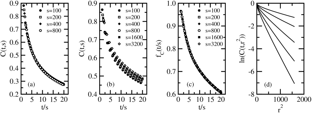
with $b^{\prime}>0$. In fact, this extended scaling form is only needed for dynamical exponents $z>3$. We illustrate this in figure 1 for two different cases: $\varepsilon=0.5$ and $T=1$, yielding $z=2.5$, in panel (a), and $\varepsilon=2$ and $T=1$, yielding $z=4$, in panels (b) and (c). Whereas for $z=2.5$ one readily observes the $t/s$-scaling behaviour of simple ageing, the existence of finite-time corrections to scaling is obvious for $z=4$. After subtracting off this correction, we recover the scaling of simple ageing $C(t,s)=f_{C}(t/s)$, as shown in panel (c). We list in table 4 the values of the exponent $b^{\prime}$ of the correction term. It is natural that finite-time corrections should become increasingly important with increasing values of $z$, since the domain size $L(t)\sim t^{1/z}$ will grow more slowly for $z$ larger and scaling will set in later.

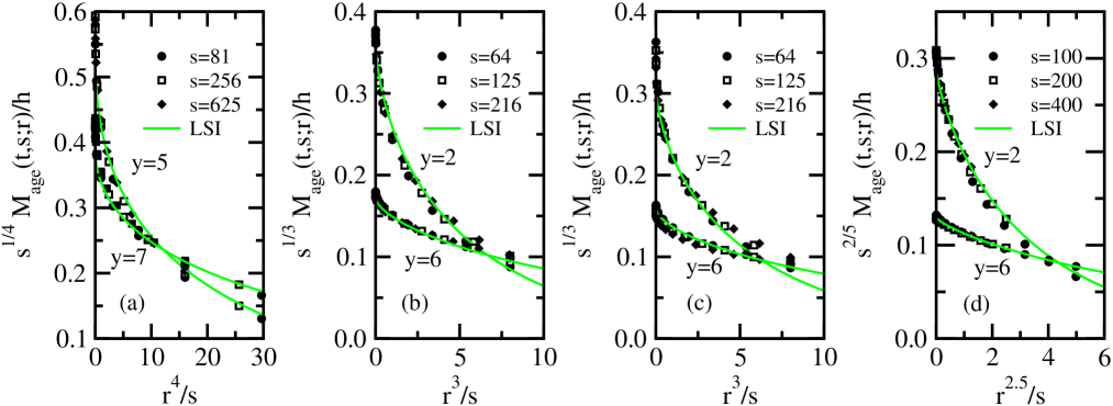
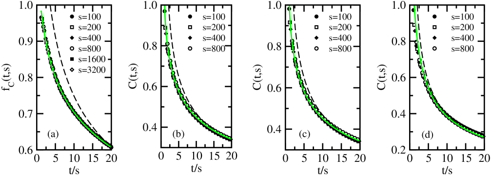
In figures 2 and 3 we show the scaling functions for the ageing part of the spatial thermoremanent magnetisation $M_{\rm age}(t,s;\boldsymbol{r})$ and the autocorrelation function $C(t,s)$ for several combinations of $T$ and $\varepsilon$. The observation of scaling of $M_{\rm age}$ as a function of $|\boldsymbol{r}|^{z}/s$ for $y=t/s$ fixed and with $z$ given by (3) with $\epsilon=\varepsilon$ gives a further confirmation for this dynamical exponent, see figure 2. We point out that the consideration of the spatio-temporal response allows for a much more demanding test of dynamical scaling than is possible by merely considering the autoresponse alone. Our results hence strengthen the conclusions of a simple power-law scaling in the disordered Ising model reached earlier [13, 14, 16]. Our finding that the deviations from dynamical scaling seen in the raw data of the autocorrelation [16, 24, 4] can be explained in terms of a conventional finite-time correction makes it clear that more exotic proposals such as ‘superageing’ as proposed in [24] are not required. In any case, any evidence for ‘superageing’ would have to argue against general theoretical arguments [25], which use basic constraints from probability to assert that superageing is incompatible with scaling, before it could be considered to be conclusive. Furthermore, our data suggest a stronger universality in that not only the dynamical exponent $z=2+\varepsilon/T$ but also the form of the entire scaling functions appear to depend merely on the ratio $\varepsilon/T$ but not on these two control parameters separately. We illustrate this in figure 4, where data for both the spatio-temporal response and the autocorrelator in the two cases $T=\varepsilon=1$ and $T=\varepsilon=0.5$ are shown, which according to (3) should give the same dynamical exponent $z=3$. Remarkably, not only the ageing autocorrelation and autoresponse exponents indeed agree within the numerical precision of the data, but also the scaling functions are compatible with each other, up to normalisation (the non-universal amplitudes in figure 4a was changed appropriately). This is a strong indication that the universality class of the non-equilibrium kinetics of the disordered Ising model should not depend on $T$ and $\varepsilon$ separately but rather only on the dimensionless ratio $\varepsilon/T$. Of course, this observation cannot be explained in a ‘superageing’ scenario that would be incompatible with a simple scaling law $L(t)\sim t^{1/z}$ and with the well-accepted physical idea that in phase-ordering the domain size should be the only relevant length scale [1]. Third, when considering the asymptotic fall-off of the scaling functions, we find slightly negative values of the exponent $\beta=\lambda_{C}-\lambda_{R}$, see table 4. More precise data would be needed to clarify whether these results are significantly different from $\beta=0$, as one obtains in pure systems [1, 26, 11].

[width=8.5cm]Ising_des_espace_figure4.eps

Figure 4: Comparison of the scaling functions of the cases $\varepsilon=1,T=1$ (filled symbols) and $\varepsilon=0.5,T=0.5$ (open symbols). In (a) the space-time integrated response is shown for $y=2$ (upper curve) and $y=6$ (lower curve). In (b) the autocorrelator is shown. The non-universal amplitudes have been changed appropriately.

Critical exponents and parameters of LSI for the different values of $\varepsilon$ and $T$ for the integrated response function. $\varepsilon$ $T$ $z$ $a=a^{\prime}$ $\lambda_{R}/z$ $\alpha$ $\beta$ $r_{0}$ $r_{1}$ $0.5$ $1.0$ $2.5$ $0.40(3)$ $0.61(1)$ $0.24(2)$ $-0.10(5)$ $0.0064(1)$ $~{}~{}\,0.0025(2)$ $0.5$ $0.5$ $3.0$ $0.33(5)$ $0.51(1)$ $0.20(2)$ $-0.06(7)$ $0.0049(1)$ $~{}~{}\,0.005(2)$ $1.0$ $1.0$ $3.0$ $0.33(5)$ $0.51(1)$ $0.20(1)$ $-0.06(7)$ $0.00575(2)$ $-0.02(1)$ $2.0$ $1.0$ $4.0$ $0.25(2)$ $0.33(1)$ $0.15(2)$ $-0.04(10)$ $0.0365(1)$ $-0.035(2)$ Critical exponents and parameters of LSI for the different values of $\varepsilon$ and $T$ for the autocorrelation function. $\varepsilon$ $T$ $z$ $\lambda_{C}/z$ $c_{1}$ $\rho$ $(2\beta+d-\lambda_{C})/z$ $\nu$ $c_{2}$ $b^{\prime}$ $0.5$ $1.0$ $2.5$ $0.570(5)$ $1.51(2)$ $0.14(2)$ $0.16(1)$ $0.31(2)$ $1.72(1)$ – $0.5$ $0.5$ $3.0$ $0.490(5)$ $1.48(1)$ $0.16(3)$ $0.14(1)$ $0.35(2)$ $1.30(1)$ – $1.0$ $1.0$ $3.0$ $0.490(5)$ $1.48(1)$ $0.16(3)$ $0.14(1)$ $0.36(2)$ $1.30(1)$ – $2.0$ $1.0$ $4.0$ $0.320(5)$ $1.62(2)$ $0.15(2)$ $0.15(1)$ $0.48(2)$ $1.12(1)$ $0.075$

After these preparations, we can now consider the form of the scaling functions and compare our data with the LSI-predictions (2) and (11,13), respectively. For the space-time response function, the four panels in figure 2 clearly show an excellent agreement. Since (2) does not depend on the initial correlations, any assumption about the initial correlations only enters via the values of the parameters $\alpha,\beta$ which must the same as for the autocorrelation. This is the first time that Galilei-invariance generalised to $z\neq 2$ [8, 11] could be directly confirmed for a model with an underlying non-linear Langevin equation. It is non-trivial that a single theory is capable to reproduce the shapes of the scaling functions for values of the dynamical exponents which vary considerably. Together with our previous test [16] of LSI for the autoresponse function in this model, this is strong evidence that LSI captures the essence of the dynamical scaling behaviour of the linear response.

On the other hand, tests of LSI for the autocorrelation functions are conceptually more difficult. First, we consider a fully disordered initial state, as suggested by the naïve comparison with the lattice model. In figure 3 we compare with the prediction (11), with parameter estimates listed in table 4. Clearly, one has at best a qualitative agreement and particular for smaller values of $y=t/s$, the data deviate strongly from the curve (11). Should one take this as a bona fide indication that LSI could not describe the ageing of the $2D$ disordered Ising model? We have already recalled above the general arguments [21] which suggest that ageing only sets in for time differences $\tau=t-s\sim s^{\zeta}$, with $s\gg t_{\rm micro}$ and $0<\zeta<1$. This implies that the form of the scaling function should rather be related to the ‘initial’ correlator $C(s+\tau,s;\boldsymbol{r})$. In figure 1d we show that the leading space-dependent behaviour of the equal-time correlator $C(s,s;\boldsymbol{r})$ that strongly deviates from a totally uncorrelated correlator which means that the system had time enough to build up strong spatially long-range correlations. We have also checked that the leading $\boldsymbol{r}$-dependence is also recovered in space-time-dependent correlators $C(t,s;\boldsymbol{r})$, with $y=t/s=2$ or $3$. Therefore, the assumed initial correlator eq. (12) appears to be in good agreement with direct numerical data for the asymptotic behaviour of the ‘initial’ correlator. That form is quite reminiscent to the well-known analytic forms found in phase-ordering kinetics of pure systems (where $z=2$) [1] and is one of the most simple generalisations to $z\neq 2$. We see from figure 3 that the expression (13) for the autocorrelator $C(t,s)$ predicted by LSI agrees nicely with the data and also confirm eq. (14). This is the first time that a consequence of the factorisation of the four-point response function is confirmed in a system with a non-linear Langevin equation. Refining the chosen form (12) of the initial correlator will merely lead to small corrections to (13), in particular for $y\to 1$.

4 Summary

1. Taking into account strong finite-time corrections to scaling, we find simple ageing behaviour for both the two-time responses and correlators of the $2D$ disordered Ising model. No trace of a ’superageing’ behaviour is seen.
2. Not only the dynamical exponent $z=z(T,\varepsilon)$ as given by (3), but also the universal form of the scaling functions only depends on the ratio $\varepsilon/T$.
3. The agreement of the space-time response predicted by LSI with the numerical data constitutes the first direct confirmation of Galilei-invariance generalised to $z\neq 2$ in a non-linear model of ageing.
4. The precise scaling form of the autocorrelator $C(t,s)$ does depend on the initial space-time correlator at the onset of the ageing regime. While the usual hypothesis of a fully uncorrelated order-parameter does not describe the data, the asymptotic form eq. (12) leads to a good agreement between LSI and the data. In this way, we have confirmed for the first time the factorisation of the $2n$-point response functions, characteristic of LSI with $z\neq 2$ [8], in a non-linear model of ageing.

The numerical results presented in this letter are strong evidence in favour of the existence of a local scale-invariance of the ‘deterministic’ part of the stochastic Langevin equation which describes the phase-ordering kinetics of the $2D$ disordered Ising model. This is the first time that LSI could be confirmed for both correlators and responses in a non-linear model with a dynamical exponent $z\neq 2$. Further tests of LSI in different systems with $z\neq 2$ would be welcome.