CPHT-RR069.0707

The Phase Structure of Higher-Dimensional Black Rings and Black Holes
Roberto Emparan^a,b, Troels Harmark^c, Vasilis Niarchos^d,
Niels A. Obers^c, María J. Rodríguez^b
aInstitució Catalana de Recerca i Estudis Avançats (ICREA)
^bDepartament de Física Fonamental, Universitat de Barcelona,
Diagonal 647, E-08028 Barcelona, Spain
^cThe Niels Bohr Institute, Blegdamsvej 17, 2100 Copenhagen Ø, Denmark
^dCentre de Physique Théorique, École Polytechnique, 91128 Palaiseau, France
Unité mixte de Recherche 7644, CNRS

emparan@ub.edu, harmark@nbi.dk, niarchos@cpht.polytechnique.fr, obers@nbi.dk, majo@ffn.ub.es

Abstract

We construct an approximate solution for an asymptotically flat, neutral, thin rotating black ring in any dimension $D\geq 5$ by matching the near-horizon solution for a bent boosted black string, to a linearized gravity solution away from the horizon. The rotating black ring solution has a regular horizon of topology $S^{1}\times S^{D-3}$ and incorporates the balancing condition of the ring as a zero-tension condition. For $D=5$ our method reproduces the thin ring limit of the exact black ring solution. For $D\geq 6$ we show that the black ring has a higher entropy than the Myers-Perry black hole in the ultra-spinning regime. By exploiting the correspondence between ultra-spinning black holes and black membranes on a two-torus, we take steps towards qualitatively completing the phase diagram of rotating blackfolds with a single angular momentum. We are led to propose a connection between MP black holes and black rings, and between MP black holes and black Saturns, through merger transitions involving two kinds of ‘pinched’ black holes. More generally, the analogy suggests an infinite number of pinched black holes of spherical topology leading to a complicated pattern of connections and mergers between phases.

1 Introduction

In this paper we explore the possible black hole solutions of the Einstein equations $R_{\mu\nu}=0$ in six or more dimensions. Our understanding of the black hole phases in five dimensions has advanced greatly in recent years. In addition to the Myers-Perry (MP) black holes [1], there exist rotating black rings [2, 3] and multi-black hole solutions like black-Saturns and multi-black rings [4, 5, 6, 7]. The latter have been constructed using inverse-scattering techniques [8, 9, 10, 11], which have also yielded a black ring solution and multi-black rings with two independent angular momenta [12, 13]. There exist furthermore algebraic classifications of spacetimes [14, 15, 16, 17], theorems on how to determine uniquely the black hole solutions with two symmetry axes [18, 19] and further solution generating techniques [23]. In fact, it is possible that essentially all five-dimensional black holes (up to iterations of multi-black rings) with two axial Killing vectors have been found by now. Parallel to this progress, the phase diagram of black holes and black branes in Kaluza-Klein (KK) spaces is also being mapped out with increasing level of precision (see e.g. the reviews [24, 25] and the recent work [26]).

In contrast to these advances, asymptotically flat vacuum solutions with an event horizon in more than five dimensions remain largely a terra incognita, only known with certainty to be inhabited by the MP solutions. Our aim is to begin to chart this landscape. For reasons of simplicity, we shall confine ourselves to vacuum solutions, $R_{\mu\nu}=0$, with angular momentum in only one of the several independent rotation planes. However, our methods and many of our conclusions should readily extend to more general situations.

One of the main results of this paper is the construction of an approximate solution for an asymptotically flat, neutral, thin rotating black ring in any dimension $D\geq 5$ with horizon topology $S^{1}\times S^{D-3}$. The method we will employ is the one of matched asymptotic expansion [27, 28, 29, 30, 26]. Our particular construction follows primarily the approach of [27]. First we find the metric of a thin black ring in the linearized approximation to gravity sourced by the energy-momentum tensor of an infinitely thin rotating ring. Then we obtain the near-horizon metric by solving exactly the field equations to find the perturbation of a boosted black string describing the bending of the string into a circular shape. We finally match the two solutions in the overlap zone, thereby completing the solution for a thin rotating black ring. An important result of this exercise is that the perturbed event horizon remains regular. As a further check of our method, we show that in five dimensions our results for thin black rings are in agreement with the thin ring limit of the exact rotating black ring metric.

In the process of constructing the black ring solution, we find that the absence of naked singularities requires a zero-pressure condition that corresponds to balancing the string tension against the centrifugal repulsion. This is an example of how General Relativity encodes the equations of motion of black holes as regularity conditions on the geometry.

From the approximate rotating black ring solution we obtain the asymptotic properties of the area function $\mathcal{A}(M,J)$ at large spin and fixed mass, i.e. at the ultra-spinning regime. Remarkably, this central result can be obtained with surprisingly little effort. The limiting form of the function $\mathcal{A}(M,J)$ follows almost immediately from the assumption that a rotating thin black ring is well approximated as a boosted black string bent into a circle of large radius $R$. The extra ingredient we need is the zero-pressure condition that fixes the boost to a precise value.

From the area function $\mathcal{A}(M,J)$ for thin rotating black rings we find that the entropy goes like

$$S(M,J)\propto J^{-\frac{1}{D-4}}\;M^{\frac{D-2}{D-4}}\,,$$ (1.1)

whereas for the ultra-spinning MP black holes in $D\geq 6$,

$$S(M,J)\propto J^{-\frac{2}{D-5}}\;M^{\frac{D-2}{D-5}}\,.$$ (1.2)

These results show that in the ultra-spinning regime of large $J$ for fixed mass $M$ the rotating black ring has higher entropy than the MP black hole.

The other main results of this paper concern the general phase diagram of asymptotically flat neutral rotating black holes in six and higher dimensions. To gain insight into this problem we exploit a connection between, on one side, black holes and black branes in KK spacetimes and, on the other side, higher-dimensional rotating black holes. This connection was identified in [31], where it was argued that a form of the Gregory-Laflamme instability of black branes [32, 25], and the ensuing phases with non-uniform horizons [33, 34] (see also [35, 36, 37, 38]), arise naturally in the ultra-spinning regime of black holes in six or more dimensions. We can therefore use the known phase structure of the solutions on a KK two-torus to take steps towards completing the phase diagram of asymptotically flat rotating black holes. Then the extension of the curves $\mathcal{A}(M,J)$ to all $J$ at a qualitative level, and the inclusion of other new features of the phase diagram, is a matter of well-motivated analogies, using the basic idea in [31].

Employing this analogy, we develop further the conjecture in [31] that proposed the existence of ‘pinched’ black holes with spherical topology. We find a natural way to fit them in the phase diagram, and connect them to black rings and black Saturns through merger transitions.

In this paper, we do not claim to have the complete phase structure of higher-dimensional black holes, even in the case with a single rotation. Besides the uncertainties in our proposed completion of known phase curves, there may be other black hole solutions (e.g., with other horizon topologies) beyond the MP solutions, the black rings, and the pinched black holes. Nevertheless, the present work is a first application of what we think is an effective approach to learning about black holes in higher dimensions, at least at a semi-quantitative level.

The outline of the paper is as follows. In section 2 we describe how viewing a black ring as a circular boosted black string easily yields the area function $\mathcal{A}(M,J)$ in the ultra-spinning regime. Section 3 outlines the perturbative construction of thin black ring solutions. The details are then developed in sections 4, 5 and 6. In particular, in section 4 we construct the thin black ring metric in the asymptotic region where the linearized approximation to gravity is valid. Then in section 5 we consider the overlap region between the asymptotic region and the near-horizon region that enables us to derive the zero-pressure equilibrium condition for thin black rings. Finally, section 6, which is technically the most involved one, considers the metric in the near-horizon region and proves that the horizon of the black string can be bent and still remain regular. Subsequently, section 7 analyzes the resulting thermodynamics for thin black rings, and compares them to MP black holes. Section 8 combines different pieces of information to make a plausible conjecture for the qualitative structure of the black hole phases in $D\geq 6$. Section 9 discusses the results and outlook of this paper. A number of appendices are also included. Appendix A presents a set of coordinates in flat space that are adapted to a circular ring. Appendices B, C and D contain technical details employed in sections 5 and 6. Appendix E shows how the known results for the five-dimensional black rings are recovered from our method. Finally, appendix F explains how to translate the results for KK phases on $\mathbb{T}^{2}$ into a form appropriate for the correspondence to rotating black holes.

Readers who are mostly interested in the phase structure of higher-dimensional black holes may skip the technical construction of thin black ring solutions in sections 3 to 6, and, after section 2, jump to sections 7 and 8.

Throughout this paper we shall denote the number of spacetime dimensions $D$ via the number $n$ of “extra” dimensions, i.e., we set

$$D=4+n\,.$$ (1.3)

This convention makes many equations a bit cleaner.

2 Thin black rings from circular boosted black strings

Black rings in $(n+4)$-dimensional asymptotically flat spacetime are solutions of Einstein gravity with an event horizon of topology $S^{1}\times S^{n+1}$. In five dimensions explicit solutions with this topology have been presented in [2]. However, the construction of analogous solutions in more than five dimensions is a considerably more involved problem that has been unsuccessful so far—for instance, for $D\geq 6$ these solutions are not contained in the generalized Weyl ansatz [22, 20, 21] since they do not have $D-2$ commuting Killing symmetries; furthermore the inverse scattering techniques of [8, 9, 10, 11] do not extend to the asymptotically flat case in any $D\geq 6$. In what follows, we will make progress towards solving this problem by constructing thin black ring solutions in arbitrary dimensions in a perturbative expansion around circular boosted black strings.

The metric of the straight boosted black string is

$$ds^{2} = -\left(1-\cosh^{2}\alpha\frac{r_{0}^{n}}{r^{n}}\right)dt^{2}-2\frac{r_{0}^{n}}{r^{n}}\cosh\alpha\sinh\alpha\,dtdz+\left(1+\sinh^{2}\alpha\frac{r_{0}^{n}}{r^{n}}\right)dz^{2}$$ (2.1)

$$+\left(1-\frac{r_{0}^{n}}{r^{n}}\right)^{-1}dr^{2}+r^{2}d\Omega_{n+1}^{2}\,,$$

where $r_{0}$ is the horizon radius and $\alpha$ is the boost parameter. In general, we will take the $z$ direction to be along an $S^{1}$ with circumference $2\pi R$, which means we can write $z$ in terms of an angular coordinate $\psi$ defined by

$$\psi=\frac{z}{R}\,,\qquad 0\leq\psi<2\pi\,.$$ (2.2)

At distances $r\ll R$, the solution (2.1) is the approximate metric of a thin black ring to zeroth order in $1/R$.

By definition, a thin black ring has an $S^{1}$ radius $R$ that is much larger than its $S^{n+1}$ radius $r_{0}$. In this limit, the mass of the black ring is small and the gravitational attraction between diametrically opposite points of the ring is very weak. So, in regions away from the black ring, the linearized approximation to gravity will be valid, and the metric will be well-approximated if we substitute the ring by an appropriate delta-like distributional source of energy-momentum. The source has to be chosen so that the metric it produces is the same as that expected from the full exact solution in the region far away from the ring. Since the thin black ring is expected to approach locally the solution for a boosted black string, it is sensible to choose distributional sources that reproduce the metric (2.1) in the weak-field regime,

$$T_{tt} = \frac{r_{0}^{n}}{16\pi G}\,\left(n\cosh^{2}\alpha+1\right)\,\delta^{(n+2)}(r)\,,$$ (2.3a)

$$T_{tz} = \frac{r_{0}^{n}}{16\pi G}\,n\cosh\alpha\sinh\alpha\,\delta^{(n+2)}(r)\,,$$ (2.3b)

$$T_{zz} = \frac{r_{0}^{n}}{16\pi G}\,\left(n\sinh^{2}\alpha-1\right)\,\delta^{(n+2)}(r)\,.$$ (2.3c)

The location $r=0$ corresponds to a circle of radius $R$ in the $(n+3)$-dimensional Euclidean flat space, parametrized by the angular coordinate $\psi$. We shall be more specific about these coordinates in later sections.

In this construction the mass and angular momentum of the black ring are obtained by integrating the energy and momentum densities,

$$M = 2\pi R\int_{\mathcal{B}^{n+2}}T_{tt}\,,$$ (2.4a)

$$J = 2\pi R^{2}\int_{\mathcal{B}^{n+2}}T_{tz}\,,$$ (2.4b)

where $\mathcal{B}^{n+2}$ intersects the ring once so $\frac{1}{\Omega_{n+1}}\int_{\mathcal{B}^{n+2}}\delta^{(n+2)}(r)=1$. Moreover, the area of the black ring is that of a boosted black string of length $2\pi R$,

$$\mathcal{A}=2\pi R\,\Omega_{n+1}\,r_{0}^{n+1}\cosh\alpha\,.$$ (2.5)

Since $g_{tz}+\tanh\alpha\,g_{zz}=0$ at the horizon $r=r_{0}$, the linear velocity of the horizon is $v_{H}=\tanh\alpha$, hence the angular velocity of the black ring in the $\psi$-direction is

$$\Omega_{H}=\frac{v_{H}}{R}=\frac{\tanh\alpha}{R}\,.$$ (2.6)

The surface gravity is the same as that of a boosted black string,

$$\kappa=\frac{n}{2r_{0}\cosh\alpha}\,.$$ (2.7)

Such a black ring is described by three parameters: $r_{0}$, $R$ and $\alpha$ (see Refs. [39, 40] for further details on boosted black strings and their thermodynamics). More physically, we can take the parameters to be $M$, $J$, $R$, and so in principle the area is a function $\mathcal{A}(M,J,R)$. However, a black ring in mechanical equilibrium should be characterized by only two parameters: given, say, the mass and the radius, there should be only one value of the angular momentum for which the ring is in equilibrium.

It is actually easy to find the dynamical balance condition that relates the three parameters. We are approximating the black ring by a distributional source of energy-momentum. The general form of the equation of motion for probe brane-like objects has been determined in [41]. In the absence of external forces it takes the form

$${K_{\mu\nu}}^{\rho}T^{\mu\nu}=0\,,$$ (2.8)

where the indices $\mu,\nu$ are tangent to the brane and $\rho$ is transverse to it. The second fundamental tensor ${K_{\mu\nu}}^{\rho}$ extends the notion of extrinsic curvature to submanifolds of codimension possibly larger than one. The extrinsic curvature of the circle is $1/R$, so a circular linear distribution of energy-momentum of radius $R$ will be in equilibrium only if

$$\frac{T_{zz}}{R}=0\,,$$ (2.9)

i.e., for finite radius the pressure tangential to the circle must vanish. Hence, for our thin black ring with source (2.3), the condition that the ring be in equilibrium translates into a very specific value for the boost parameter

$$\sinh^{2}\alpha=\frac{1}{n}\,.$$ (2.10)

Then, eqs. (2.4) and (2.5) become

$$M = \frac{\Omega_{n+1}}{8G}\,R\,r_{0}^{n}(n+2)\,,$$ (2.11a)

$$J = \frac{\Omega_{n+1}}{8G}\,R^{2}\,r_{0}^{n}\sqrt{n+1}\,,$$ (2.11b)

$$\mathcal{A} = \Omega_{n+1}\,2\pi R\,r_{0}^{n+1}\sqrt{\frac{n+1}{n}}\,.$$ (2.11c)

Notice that an equivalent but more physical form of the equilibrium equation (2.10) is

$$R=\frac{n+2}{\sqrt{n+1}}\frac{J}{M}\,.$$ (2.12)

We see that the radius grows linearly with $J$ for fixed mass.

In principle we can eliminate $r_{0}$ and $R$ from (2.11c) to express $\mathcal{A}$ as a function of $M$ and $J$. This relation is one of the main results in this paper and it will be studied in detail later in section 7. But before that, there are two issues in our analysis that demand further scrutiny.

First, the above reasoning relies crucially on the assumption that when the boosted black string is curved, the horizon remains regular. To verify this point, and also to obtain a metric for the thin black ring, we shall solve the equations and construct an approximate solution for $r_{0}\ll R$ using a matched asymptotic expansion. This is done in sections 3 to 6.

Second, the black ring must be a solution to the source-free Einstein vacuum equations, and so the point may be raised that our derivation of the equilibrium condition (2.9) is based only on the properties of (distributional) sources. After all, in the exact five-dimensional black ring solution of [2], the equilibrium condition was not derived from any equation such as (2.8), but instead by demanding the absence of singularities on the plane of the ring outside the horizon. We will see that the use of a matched asymptotic expansion allows us to produce a similar proof of (2.9): whenever $n\sinh^{2}\alpha\neq 1$ with finite $R$, the geometry backreacts creating singularities on the plane of the ring. These singularities admit a natural interpretation. Since (2.8) is a consequence of the conservation of the energy-momentum tensor, when (2.9) is not satisfied there must be additional sources of energy-momentum. These additional sources are responsible for the singularities in the geometry. Alternatively, the derivation of (2.9) appearing below is an example of how General Relativity encodes the equations of motion of black holes as regularity conditions on the geometry.

The idea that thin black rings should be well approximated by boosted black strings is certainly not new. The black string limit of five-dimensional black rings was first made explicit in [42], where the condition $T_{zz}=0$ at equilibrium was also noticed—but the connection with (2.8) was missed. An attempt to describe thin black rings in higher dimensions with the use of boosted black strings appeared in [39], where the authors correctly predicted the existence of black rings in $D\geq 6$. They also attempted to determine the equilibrium boost of the black string by maximizing the entropy with respect to the boost. This approach is clearly different from the one here, which is instead based on mechanical equilibrium, and leads to incorrect dynamics. Even in the limit of very large number of dimensions, where the results of [39] simplify, maximization of the entropy predicts $\frac{J}{MR}\to\frac{1}{\sqrt{2n}}$ instead of the correct $\frac{J}{MR}\to\frac{1}{\sqrt{n}}$ (see eq. (2.12)). The mechanical viewpoint was advocated in [43], where a simple Newtonian model was shown to reproduce the correct equilibrium in 5D and so ref. [43] independently pointed out the possibility of equilibrium configurations of thin rotating black rings in all $D\geq 5$. However, the model does not capture correctly all the relativistic ring dynamics, and would predict a value of the boost in conflict with $T_{zz}=0$ in $D\geq 6$, so the authors of [43] chose not to make any quantitative predictions.

3 Matched asymptotic expansions

Our aim is to construct approximate solutions for thin black rings following a systematic approach that, in principle, allows to proceed iteratively by starting from a limit where the solution is known and then correcting it in a perturbative expansion. The method was first used in [27] to construct black holes localized on a KK circle, and then subsequently refined and extended in the same context in [28, 29, 30, 26]. Ref. [28] provides a lucid description of the method.

The basic idea is that, in a problem with two widely separated scales, we can try to find approximate solutions to the equations in two zones and match them at an intermediate zone where both approximations are valid. In our problem, the two scales are $r_{0}$ and $R$. We will first consider an asymptotic zone at large distances from the black ring, $r\gg r_{0}$, where the field can be expanded in powers of $r_{0}$. Next we will consider the near-horizon zone that lies at scales much smaller than the ring radius, $r\ll R$. In this zone the field is expanded in powers of $1/R$. At each step, the solution in one of the zones is used to provide boundary conditions for the field in the other zone, by matching the fields in the ‘overlap’ zone $r_{0}\ll r\ll R$ where both expansions are valid.

In more detail, the first few steps in this construction, which are the ones that we develop in this paper, proceed as follows:

1. In the zeroth order step, we consider the solution in the near-horizon zone to zeroth order in $1/R$, i.e., we take a boosted black string of infinite length, $R\to\infty$. Relating the parameters $r_{0}$, $R$ of the black string to the asymptotic mass and angular momentum of the black ring is most simply done using the analogue of Gauss’ law in General Relativity, namely, Stokes’ theorem applied to the Komar integrals for $M$ and $J$.

2. Then we solve the Einstein equations in the linearized approximation around flat space, for a source of the right form — in this case a circular distribution of a given mass and momentum density. The linearized approximation is an expansion to first order in $r_{0}^{n}\propto GM/R$, valid for $r_{0}\ll r$. The linearized solution is completely determined (up to gauge transformations) by the sources and the boundary conditions of asymptotic flatness.

3. Next we focus on the near-horizon region of the ring. The goal is to find the linear corrections to the metric of a boosted black string for a perturbation that is small in $1/R$; in other words, we analyze the geometry of a boosted black string that is now slightly curved into a circular shape. To find these corrections, one must solve a set of homogeneous equations, and therefore boundary conditions must be provided. The matching to the solution of the previous step in the overlap region $r_{0}\ll r\ll R$ provides boundary conditions at large $r$ (with due care to the gauge choices in the two regions). In addition, one must also pay attention to the regularity conditions at the horizon $r\to r_{0}$.

4. The near-horizon metric can now be used to fix the integration constants that appear when one solves for the next-to-linearized order corrections at large distances. We shall not solve this step, since, as in step 0, there is always a simpler way to obtain the physical asymptotic magnitudes $M$ and $J$ to this order [27]: the corrections to the metric near the horizon determine the corrections to the area $\cal A$, temperature $T$, and angular velocity $\Omega_{H}$. By using the Smarr relations and the first law, we can immediately deduce the corrections to the mass and angular momentum. In principle, these are measured at infinity, but the Smarr relations and the first law can give the required information since they use implicitly the equations of motion.

Step 0 has been discussed already in section 2. The relation $\mathcal{A}(M,J)$ to leading order, following from (2.11), gives the asymptotic form of the phase curve of thin black rings. Simple as this is, it nevertheless gives us non-trivial information, as it tells us e.g., whether MP black holes or black rings dominate the entropy at large spins. Step 1 will be solved in sections 4 and 5. Step 2 is then developed in section 6. Step 3, discussed at the end of section 6, gives the leading order corrections to the entropy curve ${\cal A}(M,J)$. We will actually find that these corrections vanish for thin black rings in six or more dimensions.

4 Black rings in linearized gravity

We want to find the solution that describes a thin black ring, with $S^{n+1}$ radius $r_{0}$ much smaller than its $S^{1}$ radius $R$, in the region $r\gg r_{0}$ where the linearized approximation to gravity should be valid.

We solve the linearized Einstein equations in transverse gauge,

$$\Box\bar{h}_{\mu\nu}=-16\pi GT_{\mu\nu}\,$$ (4.1)

with $\bar{h}_{\mu\nu}=h_{\mu\nu}-\frac{1}{2}hg_{\mu\nu}$ and $\nabla_{\mu}\bar{h}^{\mu\nu}=0$. Writing the $(n+3)$-dimensional Euclidean flat space metric in bi-polar coordinates

$$ds^{2}(\mbox{${\mathbb{E}}^{n+3}$})=dr_{1}^{2}+r_{1}^{2}d\Omega^{2}_{n}+dr_{2}^{2}+r_{2}^{2}d\psi^{2}$$ (4.2)

we take the equivalent ring source to lie at $r_{1}=0$ and $r_{2}=R$. Locally the source must reproduce a boosted black string, with non-zero energy density $T_{tt}$ and angular momentum density $T_{t\psi}=R\,T_{tz}$ as in (2.3). Finding the solution valid at all $r_{1}$ and $r_{2}$ with non-zero $T_{\psi\psi}=R^{2}\,T_{zz}$ is not easy, so we shall assume that the equilibrium condition $T_{\psi\psi}=0$ is satisfied. In this case the general form of the metric is

$$ds^{2}=(-1+2\Phi)dt^{2}-2Adtd\psi+\left(1+\frac{2}{n+1}\Phi\right)ds^{2}(\mbox{${\mathbb{E}}^{n+3}$})\,,$$ (4.3)

where $\Phi$ and $A$ depend only on $r_{1},r_{2}$ and are sourced respectively by $T_{tt}$ and $T_{t\psi}$. Their equations are actually very simple: away from the source, $\Phi$ must solve the scalar Laplace equation, and $A$ the Maxwell equation for a gauge potential $A_{\mu}dx^{\mu}=Ad\psi$. The solutions for the appropriate distributional sources have already been constructed in [44] (see [45] for further details). For the scalar potential we have

$$\Phi=\frac{4GM}{(n+2)\Omega_{n+2}}\int_{0}^{2\pi}d\psi\,\frac{1}{\left(r_{1}^{2}+(R\cos\psi-r_{2})^{2}+R^{2}\sin^{2}\psi\right)^{(n+1)/2}}$$ (4.4)

and for the vector potential $A$,

$$A=\frac{8GJ}{(n+1)\Omega_{n+2}R}\int_{0}^{2\pi}d\psi\,\frac{r_{2}\cos\psi}{\left(r_{1}^{2}+(R\cos\psi-r_{2})^{2}+R^{2}\sin^{2}\psi\right)^{(n+1)/2}}\,.$$ (4.5)

These integrals take simple forms only when $n$ is odd [44], while for even $n$ they involve elliptic functions [45]. Nevertheless, they can be approximately calculated both in the asymptotic region $r_{1},r_{2}\gg R$ and in the ‘overlap’ zone $r_{1},\,r_{2}-R\ll R$. The values at asymptotic infinity

$$\Phi\to\frac{8\pi GM}{(n+2)\Omega_{n+2}}\frac{1}{\left(r_{1}^{2}+r_{2}^{2}\right)^{\frac{n+1}{2}}}\,,\qquad A\to\frac{8\pi GJ}{\Omega_{n+2}}\frac{r_{2}^{2}}{\left(r_{1}^{2}+r_{2}^{2}\right)^{\frac{n+3}{2}}}$$ (4.6)

have been used to normalize the potentials in terms of the ADM mass and angular momentum, $M$ and $J$. Since the latter can also be computed using Komar integrals, if we move the integration surface from infinity towards the vicinity of the source (2.3), the relations (2.11) follow easily.

5 The overlap zone: deriving the zero-tension condition

In the previous section we found the linearized solution with arbitrary mass and angular momentum, and zero tension. Finding the solution with a source for tension is more complicated, but the task becomes much easier if one restricts to the overlap zone $r_{0}\ll r_{1},\,r_{2}-R\ll R$. In this regime we are studying the effects of locally curving a thin black string into an arc of constant curvature radius $R$. We shall prove that a regular solution is possible only if $T_{\psi\psi}=0$.

5.1 Adapted coordinates

In order to study the effect of curving the string into a circle of radius $R$, it is very convenient to use adapted coordinates, i.e., coordinates that correspond to equipotential surfaces of the field of a circular source. One can work out a system of such coordinates valid both in the asymptotic and near-ring zones, and this was indeed the approach taken in [27] using the coordinate system and ansatz introduced in [46]. While a similar exercise can be carried out as well for this problem, see appendix A, it is technically quite involved and in general impractical. A simpler method goes as follows.

We work directly in the region $r\ll R$, to leading order in $1/R$. In order to find coordinates for flat space so that $r=0$ is an arc of ring of radius $R$, we seek a metric such that:

• The metric is Riemann-flat to order $1/R$.

• The curve $r=0$ on the ring plane $\theta=0,\pi$ has constant extrinsic curvature radius $R$.

We will also require that surfaces of constant radial coordinate $r$ are equipotential surfaces of the Laplace equation for a delta-function source at $r=0$:

• $\nabla^{2}r^{-{n}}=0$.

Let us then make the ansatz

$$ds^{2}=\left(1+A(\theta)\frac{r}{R}\right)dz^{2}+\left(1+B(\theta)\frac{r}{R}\right)dr^{2}+\left(1+C(\theta)\frac{r}{R}\right)r^{2}(d\theta^{2}+\sin^{2}\theta d\Omega_{n}^{2})\,.$$ (5.1)

Riemann flatness requires that $A(\theta)=A\cos\theta$, with constant $A$. Also, up to irrelevant additive constants, it requires $B(\theta)=C(\theta)=B\cos\theta$. Then, $\nabla^{2}r^{-n}=0$ implies $A=-nB$. The correct curvature radius $R$ is obtained for $A=2$.

Thus, the flat space metric, to first order in $1/R$, is

$$ds^{2}(\mbox{${\mathbb{E}}^{n+3}$})=\left(1+\frac{2r\cos\theta}{R}\right)dz^{2}+\left(1-\frac{2}{n}\frac{r\cos\theta}{R}\right)\left(dr^{2}+r^{2}d\theta^{2}+r^{2}\sin^{2}\theta d\Omega_{n}^{2}\right)\,.$$ (5.2)

The relation between this metric and (4.2) is studied in appendix A.

In these coordinates, we consider a general distributional linear source of mass, momentum and tension,

$$T_{tt} = \frac{n(n+2)}{n+1}\;\mu\;\frac{r_{0}^{n}}{16\pi G}\;\delta^{(n+2)}(r)\,,$$ (5.3a)

$$T_{tz} = n\,p\,\frac{r_{0}^{n}}{16\pi G}\;\delta^{(n+2)}(r)\,,$$ (5.3b)

$$T_{zz} = \frac{n(n+2)}{n+1}\;\tau\;\frac{r_{0}^{n}}{16\pi G}\;\delta^{(n+2)}(r)\,.$$ (5.3c)

This is more general than (2.3), since we allow the three components to be independent. The source is parametrized with three dimensionless quantities $\mu,\,p,\,\tau$ (conveniently normalized to simplify later results) but one of them could be absorbed in $r_{0}$. The boosted black string has

$$\frac{n(n+2)}{n+1}\mu = n\,\cosh^{2}\alpha+1\,,$$ (5.4a)

$$\frac{n(n+2)}{n+1}\tau = n\,\sinh^{2}\alpha-1\,,$$ (5.4b)

$$p = \cosh\alpha\sinh\alpha\,.$$ (5.4c)

In order to be more general, and to have a clearer notation, we choose to work with a general source and with a superfluous parameter.

5.2 Solving the equations

In the adapted coordinates (5.2), using the symmetries of the solution and appropriate gauge choices, it is possible to bring the metric corrections to the form

$$h_{tt} = f_{1}(r,\theta)\,,$$ (5.5a)

$$h_{tz} = f_{2}(r,\theta)\,,$$ (5.5b)

$$h_{zz} = f_{3}(r,\theta)\gamma_{zz}\,,$$ (5.5c)

$$h_{rr} = f_{4}(r,\theta)\gamma_{rr}\,,$$ (5.5d)

$$h_{\theta\theta} = f_{5}(r,\theta)\gamma_{\theta\theta}\,,$$ (5.5e)

$$h_{\Omega\Omega} = f_{6}(r,\theta)\gamma_{\Omega\Omega}\,,$$ (5.5f)

where $\gamma_{\mu\nu}$ is the flat space metric (5.2) to $O(1/R^{2})$ and the subindices _ΩΩ denote the coordinates for the $n$-sphere $S^{n}$. This perturbation involves six functions $f_{i}(r,\theta)$, but since we are considering a source with only $T_{tt}$, $T_{tz}$, $T_{zz}$, actually only three of the functions will be independent. Finding the complete reduction to three functions is possible but complicated. Fortunately, for our analysis we will only need to find one explicit relation among the six functions in (5.5). The argument is given in appendix B and implies

$$f_{1}-f_{3}-f_{4}-f_{5}-(n-2)f_{6}=0\,.$$ (5.6)

The off-diagonal perturbation $h_{tz}$, and hence $f_{2}$, decouples and can be found separately. Recall also that the transverse gauge condition $\nabla_{\mu}\bar{h}^{\mu}_{\nu}=0$ must be imposed. We will regard it as one more field equation.

The radial dependence of $f_{i}$ can be fixed by dimensional arguments. If we separate the zeroth and first order corrections in $1/R$ we can write

$$f_{i}(r,\theta)=\frac{r_{0}^{n}}{r^{n}}\left(f_{i}^{(0)}(\theta)+\frac{r}{R}f_{i}^{(1)}(\theta)\right)\,.$$ (5.7)

To solve for $f_{i}^{(0)}(\theta)$ note that to zeroth order in $1/R$ we are simply finding the linearized perturbation created by a straight linear distribution of mass, momentum and pressure. Then at this order the $SO(n+2)$ symmetry of the $S^{n+1}$ spheres is unbroken and therefore the $f_{i}^{(0)}$ must be constants. Using (5.3), these constants are easily found to be

$$f^{(0)}_{1} = \mu+\frac{\tau}{n+1}\,,$$ (5.8a)

$$f^{(0)}_{2} = -p\,,$$ (5.8b)

$$f^{(0)}_{3} = \tau+\frac{\mu}{n+1}\,,$$ (5.8c)

$$f^{(0)}_{4} = f^{(0)}_{5}=f^{(0)}_{6}=\frac{\mu-\tau}{n+1}\,.$$ (5.8d)

For later reference, we note that in order to pass to ‘Schwarzschild gauge’, in which $h_{\theta\theta}^{(0)}=h_{\Omega\Omega}^{(0)}=0$, we must change

$$r\to r-\frac{\mu-\tau}{2(n+1)}\frac{r_{0}^{n}}{r^{n-1}}\,.$$ (5.9)

Next we solve for $f_{i}^{(1)}(\theta)$. The $R_{tt}$ equation is

$${f_{1}^{(1)}}^{\prime\prime}+n\cot\theta\,{f_{1}^{(1)}}^{\prime}-(n-1)f_{1}^{(1)}=0\,.$$ (5.10)

We show in appendix C that the only solution of this equation that is regular on the plane of the ring, i.e., at both $\theta=0,\,\pi$, is the trivial one,

$$f_{1}^{(1)}=0\,.$$ (5.11)

The $R_{zz}$ equation for $f_{3}^{(1)}$ is the same as (5.10), so again regularity implies

$$f_{3}^{(1)}=0\,.$$ (5.12)

At this stage, we impose the Einstein equation $R_{r\theta}=0$ which takes the form

$${f_{4}^{(1)}}^{\prime}+(n-1){f_{6}^{(1)}}^{\prime}+{f_{3}^{(1)}}^{\prime}-{f_{1}^{(1)}}^{\prime}+(n-1)\cot\theta({f_{6}^{(1)}}-{f_{5}^{(1)}})-\frac{n+2}{n+1}\tau\sin\theta=0\,.$$ (5.13)

If we select the regular solutions $f_{1}^{(1)}=f_{3}^{(1)}=0$ and use (5.6), this equation becomes

$$({f_{6}^{(1)}}-{f_{5}^{(1)}})^{\prime}+(n-1)\cot\theta({f_{6}^{(1)}}-{f_{5}^{(1)}})-\frac{n+2}{n+1}\tau\sin\theta=0\,.$$ (5.14)

The function $f_{6}-f_{5}$ measures the polar distortion of the $S^{n+1}$-spheres at constant $r$, whose line element is proportional to

$$d\theta^{2}+(1+f_{6}-f_{5})\sin^{2}\theta d\Omega_{n}^{2}\,.$$ (5.15)

In general we may have $f_{6}\neq f_{5}$, but in order to avoid a conical singularity at the poles of the sphere the two functions must be equal there,

$$f_{6}(\theta=0)=f_{5}(\theta=0)\,,\qquad f_{6}(\theta=\pi)=f_{5}(\theta=\pi)\,.$$ (5.16)

In appendix C we show that this condition can only be satisfied if the inhomogeneous term in the equation (5.14) vanishes, i.e., $\tau=0$. So we find that regularity of the solution can be achieved only if

$$T_{zz}=0\,,$$ (5.17)

i.e., the tension along the ring must vanish. We have thus reproduced the result (2.9) as a condition of absence of naked singularities on the plane of the ring.

Imposing this condition, it is now easy to solve the remaining equations. Since $T_{tt}$ and $T_{tz}$ do not affect the purely spatial components of $\bar{h}_{\mu\nu}$ we must have $f_{4}^{(1)}=f_{5}^{(1)}=f_{6}^{(1)}$ and then (5.6) with (5.11), (5.12) imply

$$f_{4}^{(1)}=f_{5}^{(1)}=f_{6}^{(1)}=0\,.$$ (5.18)

Finally, the $R_{tz}$ equation

$${f_{2}^{(1)}}^{\prime\prime}+n\cot\theta\,{f_{2}^{(1)}}^{\prime}-(n-1)f_{2}^{(1)}-2np\cos\theta=0\,$$ (5.19)

is easily seen, using arguments like the ones used for (5.10), to have

$$f_{2}^{(1)}=-p\cos\theta\,$$ (5.20)

as its only regular solution.

If we use the equilibrium value of the boost (2.10) along with the relations (5.4) and collect the above results, the solution in the overlap zone $r_{0}\ll r\ll R$, in transverse gauge, is

$$g_{tt} = -1+\frac{n+1}{n}\frac{r_{0}^{n}}{r^{n}}\,,$$ (5.21a)

$$g_{tz} = -\frac{\sqrt{n+1}}{n}\frac{r_{0}^{n}}{r^{n}}\left(1+\frac{r\cos\theta}{R}\right)\,,$$ (5.21b)

$$g_{zz} = 1+\frac{1}{n}\frac{r_{0}^{n}}{r^{n}}\left(1+\frac{2r\cos\theta}{R}\right)+\frac{2r\cos\theta}{R}\,,$$ (5.21c)

$$g_{rr} = 1+\frac{1}{n}\frac{r_{0}^{n}}{r^{n}}\left(1-\frac{2}{n}\frac{r\cos\theta}{R}\right)-\frac{2}{n}\frac{r\cos\theta}{R}\,,$$ (5.21d)

$$g_{ij} = \hat{g}_{ij}\left[1+\frac{1}{n}\frac{r_{0}^{n}}{r^{n}}\left(1-\frac{2}{n}\frac{r\cos\theta}{R}\right)-\frac{2}{n}\frac{r\cos\theta}{R}\right]\,.$$ (5.21e)

where in the angular part we have a factor

$$\hat{g}_{ij}dx^{i}dx^{j}=r^{2}(d\theta^{2}+\sin^{2}\theta d\Omega^{2}_{n})\,$$ (5.22)

of a round $S^{n+1}$ of radius $r$. The metric, however, has symmetry $SO(n+1)$ and not $SO(n+2)$ since it depends explicitly on $\theta$.

One can check that the complete linearized solution of the previous section, (4.3)-(4.5), reduces to this metric in the overlap zone. To this effect, one must use the relations (2.11) between parameters, and the change of coordinates in (A.19).

For the purposes of the following section we pass to ‘Schwarzschild gauge’ (5.9),

$$r\to r-\frac{1}{2n}\frac{r_{0}^{n}}{r^{n-1}}\,,$$ (5.23)

in which the solution takes the form

$$g_{tt} = -1+\frac{n+1}{n}\frac{r_{0}^{n}}{r^{n}}\,,$$ (5.24a)

$$g_{tz} = -\frac{\sqrt{n+1}}{n}\frac{r_{0}^{n}}{r^{n}}\left(1+\frac{r\cos\theta}{R}\right)\,,$$ (5.24b)

$$g_{zz} = 1+\frac{1}{n}\frac{r_{0}^{n}}{r^{n}}\left(1+\frac{r\cos\theta}{R}\right)+\frac{2r\cos\theta}{R}\,,$$ (5.24c)

$$g_{rr} = 1+\frac{r_{0}^{n}}{r^{n}}\left(1-\frac{2n-1}{n^{2}}\frac{r\cos\theta}{R}\right)-\frac{2}{n}\frac{r\cos\theta}{R}\,,$$ (5.24d)

$$g_{ij} = \hat{g}_{ij}\left(1+\frac{1}{n^{2}}\frac{r_{0}^{n}}{r^{n-1}R}\cos\theta-\frac{2}{n}\frac{r\cos\theta}{R}\right)\,.$$ (5.24e)

6 Perturbations of the boosted black string

6.1 Setting up the near-horizon perturbation analysis

We now turn to the perturbations of the metric near the horizon. These arise when we force the field of the boosted black string to become like (5.24) at large distances, i.e., we curve the string into a circle of large but finite radius $R$. In effect, we are placing the black string in an external potential whose form at large distances can be read from (5.24), and which changes the metric $g^{(0)}_{\mu\nu}$ of the boosted black string by a small amount

$$g_{\mu\nu}=g^{(0)}_{\mu\nu}+h_{\mu\nu}\,$$ (6.1)

of order $1/R$.

For the unperturbed metric we take the boosted black string (2.1) with “critical” boost parameter (2.10),

$$g^{(0)}_{tt}=-1+\frac{n+1}{n}\frac{r_{0}^{n}}{r^{n}}\,,\qquad g^{(0)}_{tz}=-\frac{\sqrt{n+1}}{n}\frac{r_{0}^{n}}{r^{n}}\,,\qquad g^{(0)}_{zz}=1+\frac{1}{n}\frac{r_{0}^{n}}{r^{n}}$$ (6.2a)

$$g^{(0)}_{rr}=\left(1-\frac{r_{0}^{n}}{r^{n}}\right)^{-1}\,,\qquad g^{(0)}_{\theta\theta}=\hat{g}_{\theta\theta}\,,\qquad g^{(0)}_{\Omega\Omega}=\hat{g}_{\Omega\Omega}$$ (6.2b)

where $\hat{g}_{\theta\theta}$ and $\hat{g}_{\Omega\Omega}$ are the same as given in (5.22).

A general discussion of how the perturbations enter in a matched asymptotic expansion can be found in [28], so our discussion will be very succinct, referring to [28] for details. Modes are classified according to their tensorial character upon coordinate transformations of $S^{n+1}$, and each kind of tensor is then decomposed into the corresponding spherical harmonics of $S^{n+1}$. The equations for the modes decouple according to their tensor type and multipole order. We assume that the symmetry group $SO(n+1)$ of $S^{n}$ is unbroken so the only independent components are the scalars $h_{tt}$, $h_{tz}$, $h_{zz}$, $h_{rr}$, the vector $h_{r\theta}$, and the tensors $h_{\theta\theta}$, $h_{\Omega\Omega}$.

Given a scalar function, one can form vectors and tensors out of it via differentiation. For our purposes, it will suffice to consider such ‘scalar-derived’ vectors and tensors (instead of ‘pure’ vectors and tensors), which simplifies considerably the analysis—additional pure tensors, for instance, might be introduced, but they are actually not needed to solve the problem and since they decouple, they can be consistently set to zero. This is very convenient, since Ref. [28] shows that for scalar-derived perturbations an appropriate ‘no derivative gauge’ can be chosen which makes $h_{r\theta}=0$.

So, up to this point, we must deal with six functions $h_{tt}$, $h_{tz}$, $h_{zz}$, $h_{rr}$, $h_{\theta\theta}$, $h_{\Omega\Omega}$ of $r$ and $\theta$. We can still restrict significantly the form of the perturbations by considering how they arise. The metric (5.24) at large $r$ can be regarded as providing the external potential that perturbs the black string. The only perturbations that are present are proportional to $\cos\theta$, which is the Legendre polynomial $P_{\ell}(\cos\theta)$ with $\ell=1$, i.e., they are dipole perturbations. In particular, no monopoles (which would arise from a spherically symmetric component of the potential) appear. Since the different multipoles decouple, only dipoles are actually sourced and the perturbations must all be of the form

$$h_{\mu\nu}=\cos\theta\,a_{\mu\nu}(r)\,.$$ (6.3)

Moreover, it can be shown [28] that, when the tensors with $\ell=1$ are scalar-derived, we must have

$$h_{\theta\theta}=h_{\Omega\Omega}\,.$$ (6.4)

This is enough, then, to reduce the perturbations to the form

$$g_{tt}=-1+\frac{n+1}{n}\frac{r_{0}^{n}}{r^{n}}+\frac{\cos\theta}{R}a(r)\,,$$ (6.5a)

$$g_{tz}=-\frac{\sqrt{n+1}}{n}\left[\frac{r_{0}^{n}}{r^{n}}+\frac{\cos\theta}{R}b(r)\right]\,,$$ (6.5b)

$$g_{zz}=1+\frac{1}{n}\frac{r_{0}^{n}}{r^{n}}+\frac{\cos\theta}{R}c(r)\,,$$ (6.5c)

$$g_{rr}=\left(1-\frac{r_{0}^{n}}{r^{n}}\right)^{-1}\left[1+\frac{\cos\theta}{R}f(r)\right]\,,$$ (6.5d)

$$g_{ij}=\hat{g}_{ij}\left[1+\frac{\cos\theta}{R}g(r)\right]\,,$$ (6.5e)

where $\hat{g}_{ij}$ is the metric (5.22) of a $S^{n+1}$ of radius $r$.

With this ansatz, the location of the horizon will remain at $r=r_{0}$ if the perturbations are finite there. This fixes in part the choice of radial coordinate, but there still remains some gauge freedom. If we change

$$r \to r+\gamma(r)\,\frac{r_{0}}{R}\,\cos\theta\,,$$ (6.6a)

$$\theta \to \theta+\beta(r)\,\frac{r_{0}}{R}\,\sin\theta\,,$$ (6.6b)

with

$$\beta^{\prime}(r)=\frac{\gamma(r)}{r^{2}\left(1-\frac{r_{0}^{n}}{r^{n}}\right)}$$ (6.7)

then the metric remains in the form above, in particular we still have $g_{r\theta}=0$ up to order $1/R$. The condition that the horizon stays at $r=r_{0}$, i.e.,  $r_{0}\to r_{0}+O(1/R^{2})$, is

$$\gamma(r_{0})=0\,.$$ (6.8)

Under (6.6), (6.7), the perturbation variables change to

$$a(r) \to a(r)-(n+1)\,\frac{r_{0}^{n+1}}{r^{n+1}}\,\gamma(r)\,,$$ (6.9a)

$$b(r) \to b(r)-n\,\frac{r_{0}^{n+1}}{r^{n+1}}\,\gamma(r)\,,$$ (6.9b)

$$c(r) \to c(r)-\,\frac{r_{0}^{n+1}}{r^{n+1}}\,\gamma(r)\,,$$ (6.9c)

$$f(r) \to f(r)+r_{0}\,\left(2\gamma^{\prime}(r)-n\frac{r_{0}^{n}}{r^{n}}\frac{\gamma(r)}{r\left(1-\frac{r_{0}^{n}}{r^{n}}\right)}\right)\,,$$ (6.9d)

$$g^{\prime}(r) \to g^{\prime}(r)+2\frac{r_{0}}{r}\,\left(\gamma^{\prime}(r)+\frac{r_{0}^{n}}{r^{n}}\frac{\gamma(r)}{r\left(1-\frac{r_{0}^{n}}{r^{n}}\right)}\right)\,.$$ (6.9e)

There is furthermore an $r$-independent dipole gauge transformation,

$$\theta\to\theta+\beta_{0}\,\frac{r_{0}}{R}\,\sin\theta\,,$$ (6.10)

with constant $\beta_{0}$ such that everything remains unchanged except for

$$g(r)\to g(r)+2r_{0}\beta_{0}\,,$$ (6.11)

i.e.,  $g$ is redefined by an additive constant.

We might want to fix the gauge freedom (6.6) by setting one of the perturbation variables to be a specified function. It is not advisable to fix neither $a$, $b$ nor $c$ since the condition (6.8) implies that $a(r_{0})$, $b(r_{0})$, $c(r_{0})$ remain invariant and we do not know a priori what these values are. A better option is to fix $f(r)$ or $g(r)$, since their horizon values are not constrained—a simple-looking gauge choice is $f=g$. However, gauge-fixing will not be necessary nor useful in our analysis.

It will be more convenient instead to work with variables that are invariant under (6.9), such as

$${\sf A}(r) = a(r)-(n+1)\,c(r)\,,$$ (6.12a)

$${\sf B}(r) = b(r)-n\,c(r)\,,$$ (6.12b)

$${\sf F}(r) = f(r)+2r_{0}\left(\frac{r^{n+1}}{r_{0}^{n+1}}\;c(r)\right)^{\prime}-\frac{n}{\left(1-\frac{r_{0}^{n}}{r^{n}}\right)}\;c(r)\,,$$ (6.12c)

$${\sf G}^{\prime}(r) = g^{\prime}(r)+2\frac{r_{0}}{r}\left(\frac{r^{n+1}}{r_{0}^{n+1}}\;c(r)\right)^{\prime}+\frac{2}{r\left(1-\frac{r_{0}^{n}}{r^{n}}\right)}\;c(r)\,.$$ (6.12d)

We will refer to these as ‘gauge-invariant variables’, even if some of the gauge freedom has been already fixed by requiring that $g_{r\theta}=0$ and by the boundary conditions at $r\to\infty$ and $r\to r_{0}$. This way to proceed is similar to the suggestion in [47, 48] to postpone gauge-fixing as much as possible.

6.2 The master equation and its solution

Our task is to derive a ‘master equation’ for a single gauge-invariant function, with as few derivatives as possible, so that the rest of the solution (up to gauge transformations) can be obtained from the solution to the master field equation. The way we proceed is essentially similar to the one followed in [27, 28]. Ideally the master equation would be of second order, and in fact [27, 28] managed to reduce their system of equations involving $h_{tt}$, $h_{rr}$, $h_{\theta\theta}$, to a single second order ODE for the radial component of $h_{tt}$. In our case we have two additional functions from $h_{tz}$ and $h_{zz}$, which we are unable to fully decouple. As a consequence we have not managed to reduce the master equation to lower than fourth order .

While only four equations should suffice for the four gauge-invariant functions (6.12), in practice it is convenient to work with the six Einstein’s equations corresponding to the vanishing of the Ricci tensor components $R_{tt}$, $R_{tz}$, $R_{zz}$, $R_{rr}$, $R_{\theta\theta}$, and $R_{r\theta}$.

The $R_{r\theta}$ equation allows to eliminate ${\sf F}$ in terms of ${\sf A}$, ${\sf B}$, their first derivatives, and ${\sf G}^{\prime}$,

$${\sf F} = \frac{1}{n^{3}}\Biggl{[}\frac{n\Big{(}n(n+1)\,{\sf A}-2(n+1)\,{\sf B}\Big{)}}{\left(1-\frac{r_{0}^{n}}{r^{n}}\right)}+2\Big{(}n^{3}r\,{\sf G}^{\prime}-2(n+1)(r\,{\sf B}^{\prime}-\,{\sf B})+n(r\,{\sf A}^{\prime}-\,{\sf A})\Big{)}$$

$$- \frac{2}{\left(2-\frac{r_{0}^{n}}{r^{n}}\right)}\Big{(}n^{3}r\,{\sf G}^{\prime}-4(n+1)r\,{\sf B}^{\prime}+n(n+2)r\,{\sf A}^{\prime}-2(n-2)(n+1)\,{\sf B}+n\left(n^{2}-2\right)\,{\sf A}\Big{)}\Biggr{]}\,.$$

Henceforth this expression for ${\sf F}$ is plugged into the rest of the equations. Next, using the $R_{tt}$, $R_{rr}$, $R_{\theta\theta}$ equations we can eliminate ${\sf G}^{\prime}$ in terms of ${\sf A}$, ${\sf B}$, and their first derivatives,

$${\sf G}^{\prime} = \frac{1}{n^{3}}\Biggl{[}\frac{2n\left[2\,{\sf B}-n(n+2)\left((n+1)\,{\sf A}-2\,{\sf B}+r\,{\sf A}^{\prime}\right)+2(n+1)r\,{\sf B}^{\prime}\right]}{(n+1)\,r}\frac{r^{n}}{r_{0}^{n}}$$ (6.14)

$$-\frac{2(n+1)(n\,{\sf A}-2\,{\sf B})}{r\left(1-\frac{r_{0}^{n}}{r^{n}}\right)}-\frac{(n+2)\left(n\,{\sf A}^{\prime}-2(n+1)\,{\sf B}^{\prime}\right)}{(n+1)}\Biggr{]}\,.$$

This can be inserted back into (6.2) to similarly find ${\sf F}$ in terms of only ${\sf A}$, ${\sf B}$, and their first derivatives.

The remaining equations, say, from $R_{tt}$ and $R_{tz}$, reduce now to two coupled second order ODEs for ${\sf A}(r)$ and ${\sf B}(r)$. We can easily eliminate one in terms of the other, say ${\sf B}$ in terms of ${\sf A}$, as

$${\sf B} = \frac{1}{n(n+1)}\frac{r^{n}}{r_{0}^{n}}\left(1-\frac{r_{0}^{n}}{r^{n}}\right)^{2}r^{3}{\sf A}^{\prime\prime\prime}+\frac{1}{n(n+1)}\frac{r^{n}}{r_{0}^{n}}\left(1-\frac{r_{0}^{n}}{r^{n}}\right)\left(3(n+1)-(n+3)\frac{r_{0}^{n}}{r^{n}}\right)r^{2}{\sf A}^{\prime\prime}$$ (6.15)

$$+\left(2\frac{r^{n}}{r_{0}^{n}}-\frac{1}{n}\right)\left(1-\frac{r_{0}^{n}}{r^{n}}\right)r{\sf A}^{\prime}+\left(\frac{3n+2}{n}-2\frac{r^{n}}{r_{0}^{n}}\right){\sf A}\,,$$

and then find a fourth-order ODE for ${\sf A}$, which is our master equation,

$$\left(1-\frac{r_{0}^{n}}{r^{n}}\right)^{2}r^{4}{\sf A}^{\prime\prime\prime\prime}(r)+\left(1-\frac{r_{0}^{n}}{r^{n}}\right)\left[6\left(1-\frac{r_{0}^{n}}{r^{n}}\right)+4n\right]r^{3}{\sf A}^{\prime\prime\prime}(r)$$

$$+\left[5(n+1)^{2}-2(n+3)(n+2)\frac{r_{0}^{n}}{r^{n}}-(n^{2}-7)\frac{r_{0}^{2n}}{r^{2n}}\right]r^{2}{\sf A}^{\prime\prime}(r)$$

$$+(n^{2}-1)\left(2n+1-\frac{r_{0}^{2n}}{r^{2n}}\right)r{\sf A}^{\prime}(r)-(2n+1)(n^{2}-1){\sf A}(r)=0\,.$$ (6.16)

It is useful to note that if, instead, we choose ${\sf B}$ as our master variable, it satisfies exactly the same fourth-order equation (6.2) as ${\sf A}$. Also, ${\sf A}$ is given in terms of ${\sf B}$ by simply exchanging ${\sf A}\leftrightarrow{\sf B}$ in (6.15).

We have found the general solution to (6.2) through computer-aided guesswork. It can be expressed in terms of hypergeometric functions, and a convenient form for the four independent solutions is

$$u_{1}(r) = \ {}_{2}F_{1}\left(-\frac{1}{n},-\frac{n+1}{n};1;1-\frac{r_{0}^{n}}{r^{n}}\right)r\,,$$ (6.17a)

$$\ u_{2}(r) = \ {}_{2}F_{1}\left(-\frac{1}{n},\frac{n-1}{n};1;1-\frac{r_{0}^{n}}{r^{n}}\right)\frac{r_{0}^{n}}{r^{n-1}}\,,$$ (6.17b)

$$u_{3}(r) = \ {}_{2}F_{1}\left(\frac{1}{n},\frac{n+1}{n};\frac{n+2}{n};\frac{r_{0}^{n}}{r^{n}}\right)\frac{r_{0}^{n+2}}{r^{n+1}}\,,$$ (6.17c)

$$u_{4}(r) = \ {}_{2}F_{1}\left(\frac{n+1}{n},\frac{2n+1}{n};\frac{3n+2}{n};\frac{r_{0}^{n}}{r^{n}}\right)\frac{r_{0}^{2n+2}}{r^{2n+1}}\,.$$ (6.17d)

To check that the four solutions are linearly independent it suffices to compute their Wronskian in an expansion in powers of $1/r$ and see that the term at order $r^{-(4n+6)}$ is always non-zero. A general dimensional argument in [28] predicts that at leading order in $1/R$ and multipole order $\ell$ there must appear corrections $\propto r_{0}^{n+\ell+1},\,r_{0}^{2n+\ell+1},\,\dots$. Indeed, terms with powers $r_{0}^{n+2},\,r_{0}^{2n+2},\,\dots$, consistent with $\ell=1$ dipole perturbations, appear in the small $r_{0}$ expansion of all four terms in (6.17). For $n>2$ these terms are not analytic in $r_{0}^{n}\sim GM/R$.

Since both ${\sf A}$ and ${\sf B}$ satisfy the same equation, they must be of the form

$${\sf A}(r) = A_{1}\;u_{1}(r)+A_{2}\;u_{2}(r)+A_{3}\;u_{3}(r)+A_{4}\;u_{4}(r)\,,$$ (6.18a)

$${\sf B}(r) = B_{1}\;u_{1}(r)+B_{2}\;u_{2}(r)+B_{3}\;u_{3}(r)+B_{4}\;u_{4}(r)\,.$$ (6.18b)

The constants $B_{i}$ can in principle be expressed in terms of the $A_{i}$ using (6.15). Then we can also find ${\sf F}$ and ${\sf G}^{\prime}$ from (6.2) and (6.14). However, it is simpler to do this after fixing the integration constants using the boundary conditions. Eventually, the solution is fully specified by an appropriate choice of gauge, e.g.,  by fixing $c(r)$. This can not be completely arbitrary, though, since the boundary conditions at $r\to\infty$ and at the horizon also fix in part the gauge freedom. So we turn now to imposing boundary conditions.

6.3 Boundary conditions

With our choice of radial coordinate in (6.5d), and the partial gauge-fixing (6.8), the horizon, if present, remains at $r=r_{0}$. We must require that the perturbations do not make this horizon singular. In particular, the functions $a$, $b$, $c$, $f$, $g$ and their first derivatives must be finite at $r_{0}$. Then (6.12a) and (6.12b) imply that ${\sf A}$, ${\sf B}$ and their first derivatives (but not ${\sf F}$ and ${\sf G}^{\prime}$) must be finite at $r_{0}$. The hypergeometric functions ${}_{2}F_{1}\left(\alpha,\beta;\gamma;z\right)$ have logarithmic divergences at $z=1$ whenever $\alpha+\beta=\gamma$. This is the case for $u_{3}$ and $u_{4}$ in (6.17) at $r=r_{0}$, so finiteness of ${\sf A}(r_{0})$, ${\sf A}^{\prime}(r_{0})$, ${\sf B}(r_{0})$ and ${\sf B}^{\prime}(r_{0})$ requires

$$A_{3}=A_{4}=B_{3}=B_{4}=0\,.$$ (6.19)

Horizon regularity actually imposes further constraints that will be dealt with in the next subsection.

On the other hand, the large $r$-asymptotics of the functions in (6.5) are determined from Eqs. (5.24). These imply

$$a(r) = 0+O\left(r^{-n-1}\right)\,,$$ (6.20a)

$$b(r) = \frac{r_{0}^{n}}{r^{n-1}}+O\left(r^{-n-1}\right)\,,$$ (6.20b)

$$c(r) = 2r+\frac{1}{n}\frac{r_{0}^{n}}{r^{n-1}}+O\left(r^{-n-1}\right)\,,$$ (6.20c)

$$f(r) = -\frac{2}{n}r+\frac{1}{n^{2}}\frac{r_{0}^{n}}{r^{n-1}}+O\left(r^{-n-1}\right)\,,$$ (6.20d)

$$g(r) = -\frac{2}{n}r+\frac{1}{n^{2}}\frac{r_{0}^{n}}{r^{n-1}}+O\left(r^{-n-1}\right)\,,$$ (6.20e)

which, using (6.12a), (6.12b), require that

$${\sf A}(r) = -2(n+1)\,r-\frac{n+1}{n}\frac{r_{0}^{n}}{r^{n-1}}+O\left(r^{-n-1}\right)\,,$$ (6.21a)

$${\sf B}(r) = -2n\,r+O\left(r^{-n-1}\right)\,.$$ (6.21b)

This is sufficient to determine the remaining constants $A_{1}$, $A_{2}$ and $B_{1}$, $B_{2}$ in (6.18). Expanding the hypergeometric functions for large $r$, we find that (6.21) are satisfied iff

$$A_{1} = -\frac{2}{\pi}\frac{(n+1)^{2}}{n^{3}}\,\Gamma\left(\frac{1}{n}\right)^{2}\Gamma\left(-\frac{n+2}{n}\right)\sin\left(\frac{2\pi}{n}\right)\,,$$ (6.22a)

$$A_{2} = \frac{3n+4}{n(n+1)}\,A_{1}\,,\qquad B_{1}=\frac{n}{n+1}\,A_{1}\,,\qquad B_{2}=\frac{2}{n+1}\,A_{1}$$ (6.22b)

(for $n=2$ we can obtain the correct value $A_{1}=-9\pi/8$ by analytic continuation in $n$). The functions ${\sf F}$ and ${\sf G}^{\prime}$ can now be integrated explicitly from eqs. (6.2) and (6.14). The results are quoted in appendix D.

The boundary conditions (6.20) for $f$ and $g^{\prime}$ also impose restrictions on the asymptotic form of the gauge transformations (6.9), namely

$$\gamma^{\prime}(r)=O\left(r^{-n-1}\right)\,,$$ (6.23)

so

$$\gamma(r)=k\,r_{0}+O\left(r^{-n}\right)\,,$$ (6.24)

with dimensionless constant $k$. With this $\gamma$ in (6.9c), $c$ changes as

$$c\to c-k\frac{r_{0}^{n+2}}{r^{n+1}}+O\left(r^{-2n-1}\right)\,,$$ (6.25)

which does not affect the term $\propto r^{-2n+1}$ in the expansion of $c(r)$ for large $r$. So this term must be fixed once the gauge-invariant functions are determined. Using eqs. (6.12c), (6.12d), (6.20c)-(6.20e) and the solution for ${\sf F}$ and ${\sf G}^{\prime}$ at large $r$ ($e.g.$, expand eqs. (D.2) and (D.3)), it is easy to verify that the large-$r$ expansion of $c(r)$ is in fact

$$c(r)=2r+\frac{1}{n}\frac{r_{0}^{n}}{r^{n-1}}+k_{1}\frac{r_{0}^{n+2}}{r^{n+1}}-\frac{n^{2}+2n-1}{2n^{2}(n-2)}\frac{r_{0}^{2n}}{r^{2n-1}}+O\left(r^{-2n-1}\right)\,.$$ (6.26)

So one term is fixed in $c(r)$ beyond those given in (6.20), but the constant $k_{1}$, and all $O\left(r^{-2n-1}\right)$ terms, do change in general under (6.25). For $n=2$ the term $\propto r_{0}^{2n}$ is replaced by $-\frac{3}{4}\frac{r_{0}^{4}}{r^{3}}\log r$.

In addition, the asymptotic behavior of $g(r)$ removes some more gauge freedom. It requires that $g(r)+2r/n\to 0$ as $r\to\infty$, so if we fix completely the gauge symmetry (6.6), then the freedom to add a constant to $g(r)$ using (6.10) disappears.

6.4 Horizon regularity

With our choice of (6.19) the perturbation variables remain finite at the horizon $r=r_{0}$. Horizon regularity also requires that the surface gravity and the angular velocity be well-defined and uniform over the horizon [49]. To study whether it is possible to meet these conditions, we first note that the horizon is generated by the null orbits of the Killing vector field

$$\chi=\frac{\partial}{\partial t}+\Omega_{H}\frac{\partial}{\partial\psi}=\frac{\partial}{\partial t}+\Omega_{H}R\frac{\partial}{\partial z}\,,$$ (6.27)

where the angular velocity is

$$\Omega_{H} = -\frac{1}{R}\left(\frac{g_{tz}}{g_{zz}}\right)_{r_{0}}$$ (6.28)

$$= \frac{1}{\sqrt{n+1}}\frac{1}{R}\left(1+\frac{\cos\theta}{R}\left(b(r_{0})-\frac{n}{n+1}c(r_{0})\right)\right)\,.$$

If $\Omega_{H}$ is to be uniform over the horizon we must have

$$c(r_{0})=\frac{n+1}{n}b(r_{0})\,.$$ (6.29)

Furthermore, if $\chi$ is null at $r=r_{0}$ then it easily follows that $(g_{tt}+\Omega_{H}g_{tz})_{r_{0}}=0$. Together with the $\theta$-independence of $\Omega_{H}$, this requires

$$b(r_{0})=na(r_{0})\,.$$ (6.30)

Our solution of the equations, (6.18), (6.19), (6.22), determines ${\sf A}$ and ${\sf B}$ at the horizon,

$${\sf A}(r_{0}) = A_{1}\;r_{0}\;\frac{(n+2)^{2}}{n(n+1)}=a(r_{0})-(n+1)\;c(r_{0})\,,$$ (6.31a)

$${\sf B}(r_{0}) = A_{1}\;r_{0}\;\frac{n+2}{n+1}=b(r_{0})-n\;c(r_{0})\,,$$ (6.31b)

where, to avoid clutter, we do not substitute the explicit value (6.22a) of $A_{1}$. These two equations together with (6.29) completely determine the horizon values

$$a(r_{0}) = -A_{1}\;r_{0}\;\frac{n+2}{n^{2}(n+1)}\,,$$

$$b(r_{0}) = -A_{1}\;r_{0}\;\frac{n+2}{n(n+1)}\,,$$ (6.32)

$$c(r_{0}) = -A_{1}\;r_{0}\;\frac{n+2}{n^{2}}\,.$$

Happily, (6.30) is also satisfied with these values.

Next, the surface gravity $\kappa$, defined by

$$\kappa\chi^{a}=\chi^{b}\nabla_{b}\chi^{a}\,,$$ (6.33)

is

$$\kappa=\frac{n}{2}\sqrt{\frac{n}{n+1}}\frac{1}{r_{0}}\left[1-\frac{r_{0}(n+1)}{2n^{2}}\frac{\cos\theta}{R}\left(a^{\prime}(r_{0})-\frac{2b^{\prime}(r_{0})}{n}+\frac{c^{\prime}(r_{0})}{n+1}+\frac{n^{2}f(r_{0})}{(n+1)r_{0}}\right)\right]$$ (6.34)

which is uniform over the horizon only if

$$a^{\prime}(r_{0})-\frac{2b^{\prime}(r_{0})}{n}+\frac{c^{\prime}(r_{0})}{n+1}+\frac{n^{2}f(r_{0})}{(n+1)r_{0}}=0\,.$$ (6.35)

In contrast to $a(r_{0})$, $b(r_{0})$ and $c(r_{0})$, neither of the quantities entering this equation (nor $g(r_{0})$ and $g^{\prime}(r_{0})$) are invariant under (6.6) and hence are not determined until we fix the gauge. However, it is easy to check that when (6.8) holds, equation (6.35) is invariant under (6.6) and so it must be satisfied independently of the gauge choice. Although ${\sf F}$ and ${\sf G}^{\prime}$ are in general singular at $r_{0}$, using (6.4) in their solutions (D.2) and (D.3) we can readily check that $f$ and $g^{\prime}$ remain finite there. The value of $f$ at the horizon that results,

$$f(r_{0})=-r_{0}c^{\prime}(r_{0})+A_{1}r_{0}\frac{n^{2}+n-2}{n^{3}}\,$$ (6.36)

is such that using eqs. (6.12a), (6.12b) and the solution for ${\sf A}$ and ${\sf B}$, eq. (6.35) is identically satisfied and so the surface gravity is constant on the horizon. The actual values of $g(r_{0})$ and $g^{\prime}(r_{0})$ are not needed for checking the regularity of the horizon.

6.5 The complete solution

At this stage, we have given the complete explicit form for the functions ${\sf A}$, ${\sf B}$, ${\sf F}$, ${\sf G^{\prime}}$ in eqs. (6.18), (6.19), (6.22), (D.2), (D.3). Finding ${\sf G}$ requires an additional integration that we have not been able to perform explicitly in closed analytic form. But up to this quadrature, the solution is fully specified except for a choice of gauge that fixes the freedom in (6.6). From (6.12) we see that this amounts to specifying the function $c(r)$, which is only constrained to preserve the asymptotic form in (6.26) and the horizon value determined in (6.4). As explained above, once this is performed the boundary conditions imply that the symmetry (6.10) is also fixed.

A simple-looking way of fixing the gauge is to set $f=g$. In this case, since we have the explicit solution for ${\sf F}$ and ${\sf G^{\prime}}$, the function $c(r)$ is determined from the compatibility of equations (6.12c) and (6.12d). These give a second order ODE for $c(r)$, which, except for $n=1$ (see appendix E), is complicated to solve. One should show that it is possible to find solutions to this equation that satisfy the boundary conditions for $c$ at large $r$ while preserving regularity of the horizon, which may not be easy to prove. In fact this is the typical situation when one chooses the gauge a priori, without knowing whether it is actually compatible with regularity requirements.

In our approach, instead, leaving the gauge symmetry (6.6) unfixed until the end has allowed us to bypass this complication. We have managed to show that any choice of $c(r)$ with the appropriate boundary behavior produces a complete solution that is regular on and outside the horizon. For instance, we may truncate $c(r)$ to the terms shown explicitly in (6.26), and choose $k_{1}$ so that (6.4) is satisfied. Quite possibly, other choices may be simpler or more natural, so, not needing to, we shall not dwell more on this issue.

The form of our complete solution and the drastic simplifications that occur in $n=1$ (see appendix E) but not in any other $n>1$ suggest that, barring the discovery of a miraculous coordinate system, a closed exact analytic solution for a black ring exists only in five dimensions. Nevertheless, we have managed to provide a very explicit form of the approximate solution for a thin black ring in any dimension $D\geq 5$.

6.6 Properties of the corrected solution

From our results we can readily see that the area, surface gravity and angular velocity receive no modifications in $1/R$. The reason is simple: the perturbations are only of dipole type, with no monopole terms. But a dipole can not change the total area of the horizon, only its shape. This is true both of the shape of the $S^{n+1}$ as well as the length of the $S^{1}$, which can vary with $\theta$ but on average (i.e., when integrated over the horizon) remains constant. So ${\cal A}$ is not corrected. The surface gravity and angular velocity can not be corrected either. They must remain uniform on a regular horizon, so, since the dipole terms vanish at $\theta=\pi/2$, no corrections to $\kappa$ and $\Omega_{H}$ are possible. Following the arguments advanced in sec. 3, we can use the 1st law,

$$dM=\frac{\kappa}{8\pi G}d\mathcal{A}+\Omega_{H}dJ$$ (6.37)

and the Smarr formula

$$(n+1)M=(n+2)\left(\frac{\kappa{\cal A}}{8\pi G}+\Omega_{H}J\right)$$ (6.38)

to conclude that if $\mathcal{A}$, $\kappa$ and $\Omega_{H}$ are not corrected, then $M$ and $J$ cannot be corrected either. So the function $\mathcal{A}(M,J)$ obtained in (2.11) is indeed valid including the first order in $1/R$. It is interesting to observe that this conclusion could be drawn already when the asymptotic form of the metric in the overlap zone, (5.2), is seen to include only dipole terms at order $1/R$.

The length of the $S^{1}$ along $\psi$ is corrected by $c(r)$ and since $c(r_{0})\neq 0$, this length does vary at different latitudes $\theta$ on the horizon. Eqs. (6.22) and (6.4) imply that $c(r_{0})>0$, so the $S^{1}$ circle is longer along the outer rim of the ring ($\theta=0$: the pole looking towards infinity) than along its inner rim ($\theta=\pi$: looking towards the inner disk), as expected. Amusingly, the distortion of the spheres $S^{n+1}$ at constant $\psi$ on the horizon is measured by $g(r_{0})$ and therefore is a gauge-dependent property, which is only determined once a choice for $c(r)$ is made. With an appropriate gauge choice, $g(r_{0})$ can take any prescribed value— positive, negative or zero. In the latter case the $S^{n+1}$ at the horizon remain metrically round, although $g(r)$ is negative at large $r$. We have illustrated this point in appendix E.

7 Higher-dimensional black rings vs MP black holes

We now turn to study the thermodynamics of the thin black ring in the ultraspinning regime and to compare it to the exact known results for MP black holes.

Black ring

For the convenience of the reader we collect here the entire thermodynamics from (2.11), (6.28), (6.34):

$$M=\frac{\Omega_{n+1}}{8G}\,R\,r_{0}^{n}(n+2)\ ,\ \ S=\frac{\pi\,\Omega_{n+1}}{2G}R\,r_{0}^{n+1}\sqrt{\frac{n+1}{n}}\ ,\ \ T_{H}=\frac{n}{4\pi}\sqrt{\frac{n}{n+1}}\frac{1}{r_{0}}\,,$$ (7.1a)

$$J=\frac{\Omega_{n+1}}{8G}\,R^{2}\,r_{0}^{n}\sqrt{n+1}\,,\qquad\Omega_{H}=\frac{1}{\sqrt{n+1}}\frac{1}{R}\,.$$ (7.1b)

As we have seen in the previous section, these results are valid up to $O(r_{0}^{2}/R^{2})$ corrections.

MP black hole

For the MP black hole, exact results can be obtained for all values of the rotation. The two independent parameters specifying the solution are the mass parameter $\mu$ and the rotation parameter $a$, from which the horizon radius $r_{0}$ is found as the largest (real) root of the equation

$$\mu=(r_{0}^{2}+a^{2})r_{0}^{n-1}\,.$$ (7.2)

In terms of these parameters the thermodynamics take the form [1]

$$M=\frac{(n+2)\Omega_{n+2}\,\mu}{16\pi G}\,,\qquad S=\frac{\Omega_{n+2}\,r_{0}\,\mu}{4G}\,,\qquad T_{H}=\frac{1}{4\pi}\left(\frac{2r_{0}^{n}}{\mu}+\frac{n-1}{r_{0}}\right)\,,$$ (7.3a)

$$J=\frac{\Omega_{n+2}\,a\,\mu}{8\pi G}\,,\qquad\Omega_{H}=\frac{a\,r_{0}^{n-1}}{\mu}\,.$$ (7.3b)

Observe that $a=\frac{n+2}{2}\frac{J}{M}$ bears similarity with (2.12). In fact, an important simplification occurs in the ultra-spinning regime of $J\to\infty$ with fixed $M$, which corresponds to $a\rightarrow\infty$. Then (7.2) becomes

$$\mu\rightarrow a^{2}r_{0}^{n-1}$$ (7.4)

leading to simple expressions for the eqs. (7.3) in terms of $r_{0}$ and $a$, which in this regime play roles analogous to those of $r_{0}$ and $R$ for the black ring. Specifically, $a$ is a measure of the size of the horizon along the rotation plane and $r_{0}$ a measure of the size transverse to this plane [31]. In fact, in this limit

$$M\to\frac{(n+2)\Omega_{n+2}}{16\pi G}\;a^{2}r_{0}^{n-1}\,,\qquad S\to\frac{\Omega_{n+2}}{4G}\;a^{2}r_{0}^{n}\,,\qquad T_{H}\to\frac{n-1}{4\pi r_{0}}$$ (7.5)

take the same form as the expressions characterizing a black membrane extended along an area $\sim a^{2}$ with horizon radius $r_{0}$. This identification lies at the core of the ideas in [31], and we shall use it extensively in the next section. The reader may rightly wonder what happens to

$$J\to\frac{\Omega_{n+2}}{8\pi G}\;a^{3}r_{0}^{n-1}\,,\qquad\Omega_{H}\to\frac{1}{a}\,,$$ (7.6)

under this identification. Both turn out to disappear, since the black membrane limit is approached in the region near the axis of rotation of the horizon and so in the limit the membrane is static. Also observe that since eq. (7.2) is quadratic in $a$, the value (7.4), and hence also (7.5) and (7.6), are again valid up to $O(r_{0}^{2}/a^{2})$ corrections.

The transition to this membrane-like regime is signaled by a qualitative change in the thermodynamics of the MP black holes. At

$$\left(\frac{a}{r_{0}}\right)_{\rm mem}=\sqrt{\frac{n+1}{n-1}}\,,$$ (7.7)

the temperature reaches a minimum and $\left(\partial^{2}S/\partial J^{2}\right)_{M}$ changes sign. For $a/r_{0}$ smaller than this value, the thermodynamic quantities of the MP black holes such as $T$ and $S$ behave similarly to those of the Kerr solution and so we should not expect any membrane-like behavior. However, past this point they rapidly approach the membrane results.

Comparison

A meaningful comparison between dimensionful magnitudes of two solutions requires the introduction of a common scale. Then the comparison is made between dimensionless quantities obtained by factoring out this scale. Since classical General Relativity does not possess any intrinsic scale, we must take this to be one of the physical parameters of the solutions, which we conveniently take to be the mass. Thus we introduce dimensionless quantities for the spin $j$, the area $a_{H}$, the angular velocity $\omega_{H}$ and the temperature $\mathfrak{t}_{H}$ as

$$j^{n+1}=c_{j}\,\frac{J^{n+1}}{GM^{n+2}}\,,\qquad a_{H}^{n+1}=c_{a}\,\frac{\mathcal{A}^{n+1}}{(GM)^{n+2}}~{},$$ (7.8a)

$$\omega_{H}=c_{\omega}\,\Omega_{H}(GM)^{\frac{1}{n+1}}\,,\qquad\mathfrak{t}_{H}=c_{\mathfrak{t}}\,(GM)^{\frac{1}{n+1}}\,T_{H}\,,$$ (7.8b)

where the numerical constants are

$$c_{j}=\frac{\Omega_{n+1}}{2^{n+5}}\frac{(n+2)^{n+2}}{(n+1)^{\frac{n+1}{2}}}\,,\qquad c_{a}=\frac{\Omega_{n+1}}{2(16\pi)^{n+1}}(n+2)^{n+2}\left(\frac{n}{n+1}\right)^{\frac{n+1}{2}}\,,$$ (7.9a)

$$c_{\omega}=\sqrt{n+1}\left(\frac{n+2}{16}\Omega_{n+1}\right)^{-\frac{1}{n+1}}\,,\qquad c_{\mathfrak{t}}=4\pi\sqrt{\frac{n+1}{n}}\left(\frac{n+2}{2}\Omega_{n+1}\right)^{-\frac{1}{n+1}}\,.$$ (7.9b)

These are defined so that for $D=5$ ($n=1$) the conventional choice is reproduced and so that some of the formulae are simplified. Studying the entropy, or the area $\mathcal{A}$, as a function of $J$ for fixed mass is equivalent to finding the function $a_{H}(j)$. Similarly, we are interested in the quantities $\omega_{H}$ and $\mathfrak{t}_{H}$ as functions of $j$, which we take as our control parameter.

The quantities (7.8) can depend only on the dimensionless ratios $r_{0}/R$ and $r_{0}/a$ specifying the solutions. To translate this dependence in terms of the variable $j$, we can use for thin black rings and MP black holes respectively, the relations

$$j^{n+1} = 2^{-(n+2)}\left(\frac{R}{r_{0}}\right)^{n}\,,$$ (7.10a)

$$j^{n+1} = \frac{\pi}{(n+1)^{\frac{n+1}{2}}}\frac{\Omega_{n+1}}{\Omega_{n+2}}\frac{\left(\frac{a}{r_{0}}\right)^{n+1}}{1+\left(\frac{a}{r_{0}}\right)^{2}}\stackrel{{\scriptstyle a\to\infty}}{{\longrightarrow}}\frac{\pi}{(n+1)^{\frac{n+1}{2}}}\frac{\Omega_{n+1}}{\Omega_{n+2}}\left(\frac{a}{r_{0}}\right)^{n-1}\,.$$ (7.10b)

These expressions make it clear that in the regime $j\gg 1$ the black rings become thin and the MP black holes pancake along the rotation plane. According to (7.7), the onset of this behavior for the latter happens at

$$j_{\rm mem}^{{}^{n+1}}=\frac{\pi}{2n(n-1)^{\frac{n-1}{2}}}\frac{\Omega_{n+1}}{\Omega_{n+2}}\,.$$ (7.11)

We can now obtain the asymptotic phase curves for the thin black ring,

$$a_{H}=2^{\frac{n-2}{n(n+1)}}\frac{1}{j^{1/n}}\,,\qquad\omega_{H}=\frac{1}{2j}\,,\qquad\mathfrak{t}_{H}=2^{\frac{2-n}{n(n+1)}}n\,j^{1/n}\,.$$ (7.12)

Similarly, for the MP black hole in the ultra-spinning regime

$$a_{H}\to 2^{\frac{3}{n+1}}\left(\frac{\pi\Omega_{n+1}}{\Omega_{n+2}}\right)^{\frac{1}{n-1}}\frac{n^{1/2}}{(n+1)^{\frac{n+1}{2(n-1)}}}\frac{1}{j^{2/(n-1)}}~{},$$ (7.13a)

$$\omega_{H}\to\frac{1}{j}~{},\qquad\mathfrak{t}_{H}\to 2^{-\frac{3}{n+1}}\frac{(n-1)(n+1)^{\frac{n+1}{2(n-1)}}}{n^{1/2}}\left(\frac{\Omega_{n+2}}{\pi\Omega_{n+1}}\right)^{\frac{1}{n-1}}j^{2/(n-1)}\,.$$ (7.13b)

In the following we denote the results for the thin black ring with ^(r) and for the ultraspinning MP black holes with ^(h), and generally omit numerical prefactors.

Starting with the reduced area function we see that

$$a_{H}^{(r)}\sim\frac{1}{{j}^{1/n}}\,,\qquad a_{H}^{(h)}\sim\frac{1}{{j}^{2/(n-1)}}\,,$$ (7.14)

and so, for any $D=4+n\geq 6$, the area decreases faster for MP black holes than for black rings: black rings dominate entropically in the ultraspinning regime. Note also that in both cases as the dimension grows, the fall-off with $j$ becomes slower, asymptoting to $a_{H}\to j^{0}$ when $n\to\infty$ (this includes the numerical prefactor).

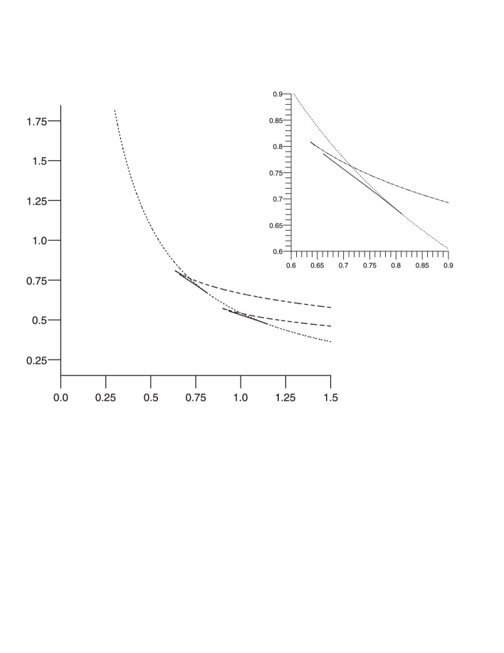
For illustration, we plot in Fig. 1 the curves in $D=7$ ($n=3$), whose asymptotic form, including numerical factors, is

$$a_{H}^{(r)}\to\frac{2^{1/12}}{j^{1/3}}\,,\qquad a_{H}^{(h)}\to\frac{2^{1/4}}{j}\,.$$ (7.15)

Figure 1: Area vs spin for fixed mass, $a_{H}(j)$, in seven dimensions. The thin curve is our result for thin black rings, valid at large $j$ and extrapolated (dashed) down to $j\sim O(1)$. The thick curve is the exact result for the MP black hole. The vertical dotted line intersects this curve at the inflection point $j=j_{\rm mem}=2^{1/4}/\sqrt{3}$, $a_{H}=\sqrt{2}$. It signals the onset at larger $j$ of membrane-like behavior for MP black holes. Eq. (7.15) gives the asymptotic form of the curves. The same qualitative features appear for all $D\geq 6$.

The ratio $\omega^{(h)}_{H}/\omega^{(r)}_{H}=2$, which holds for all $D\geq 6$, is reminiscent of the factor of 2 in Newtonian mechanics between the moment of inertia of a wheel (i.e., a ring) and a disk (i.e., a pancake) of the same mass and radius, which implies that the disk must rotate twice as fast as the wheel in order to have the same angular momentum. Irrespective of whether this is an exact analogy or not, the fact that $\omega^{(r)}_{H}<\omega^{(h)}_{H}$ is clearly expected from this sort of picture.

For the temperatures we find

$$\mathfrak{t}^{(r)}_{H}\sim j^{1/n}\ ,\ \ \mathfrak{t}^{(h)}_{H}\sim j^{2/(n-1)}\,,$$ (7.16)

so the thin black ring is colder than the MP black hole. In fact, the picture suggested above leads to the following argument: if we put a given mass in the shape of a wheel of given radius, then we get a thicker object than if we put it in the shape of a pancake of the same radius. More precisely, the spread on the rotation plane is in both cases $\sim j$, but the thickness $r_{0}$ is, for fixed mass,

$$r_{0}^{(r)}\sim j^{-1/n}\,,\qquad r_{0}^{(h)}\sim j^{-2/(n-1)}\,.$$ (7.17)

Then, the expressions in (7.16) follow immediately from the fact that the temperature is inversely proportional to the thickness $T_{H}\sim 1/r_{0}$. Moreover, observing that $T_{H}{\cal A}$ is independent of $j$ for fixed mass, the converse of this argument ‘explains’ why the black ring has higher entropy than the MP black hole of the same mass and spin.

8 Towards a complete phase diagram

The curve $a_{H}(j)$ at values of $j$ outside the domain of validity of our computation correspond to the regime where the gravitational self-attraction of the ring is important. At present, no analytical methods are known that can deal with such values $j\sim O(1)$. The precise form of the curve in this regime may require numerical solutions.

However, it is possible to complete this curve and other features of the phase diagram, at least qualitatively, by combining a number of observations and reasonable conjectures about the behavior of MP black holes at large rotation and using as input the presently known phase structure of Kaluza-Klein black holes.

8.1 GL instability of ultra-spinning MP black hole

In the ultraspinning regime in $D\geq 6$, MP black holes approach the geometry of a black membrane $\approx\mbox{${\mathbb{R}}^{2}$}\times S^{D-4}$ spread out along the plane of rotation [31]. In the previous section we have already observed that the extent of the black hole along the plane is approximately given by the rotation parameter $a$, while the ‘thickness’ of the membrane, i.e., the size of its $S^{D-4}$, is given by the parameter $r_{0}$. For $a/r_{0}$ larger than the critical value (7.7) we expect that the dynamics of these black holes is well-approximated by a black membrane compactified on a square torus $\mathbb{T}^{2}$ with side length $L\sim a$ and with $S^{D-4}$ size $\sim r_{0}$. The angular velocity of the black hole is always moderate, so it will not introduce large quantitative differences, but note that the rotational axial symmetry of the MP black holes translates into only one translational symmetry along the $\mathbb{T}^{2}$, the other one being broken.

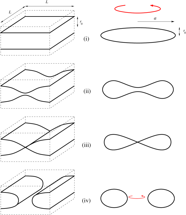
Using this analog mapping of membranes and fastly rotating MP black holes, Ref. [31] argued that the latter should exhibit a Gregory-Laflamme-type of instability. Furthermore, it is known that the threshold mode of the GL instability gives rise to a new branch of static non-uniform black strings and branes [50, 33, 34]. In correspondence with this, Ref. [31] argued that it is natural to conjecture the existence of new branches of axisymmetric ‘lumpy’ (or ‘pinched’) black holes, branching off from the MP solutions along the stationary axisymmetric zero-mode perturbation of the GL-like instability,

We intend to develop further this analogy, and draw a correspondence between the phases of black membranes and the phases of higher-dimensional black holes, as illustrated in Fig. 2. Observe that we only consider the inhomogeneities of the membrane along one of the brane directions, since the other ones do not have a counterpart for rotating black holes: they would break axial symmetry and hence would be radiated away. Other limitations of the analogy will be discussed in sec. 8.3.

Figure 2: Correspondence between phases of black membranes wrapped on a $\mathbb{T}^{2}$ of side $L$ (left) and fastly-rotating MP black holes with rotation parameter $a\sim L\geq r_{0}$ (right: must be rotated along a vertical axis): (i) Uniform black membrane and MP black hole. (ii) Non-uniform black membrane and pinched black hole. (iii) Pinched-off membrane and black hole. (iv) Localized black string and black ring.

8.2 Phase diagram of black membranes and strings on $\mathcal{M}^{D-2}\times\mathbb{T}^{2}$

Having this correspondence between the phases of the two systems, we can try to import, at least qualitatively, the known phase diagram of black membranes on $\mathcal{M}^{D-2}\times\mathbb{T}^{2}$ onto the phase diagram of rotating black objects in $\mathcal{M}^{D}$. This requires that, first, we establish the map between quantities on each side of this correspondence. Second, we must collect the available information about the former in an appropriate form.

Mapping the results for Kaluza-Klein black holes on $\mathcal{M}^{D-2}\times\mathbb{T}^{2}$ to rotating black objects in $\mathcal{M}^{D}$ requires that in both cases we choose to fix the overall scale in the same manner. For Kaluza-Klein black holes the preferred scale is usually the circumference $L$ of the asymptotic circles. For rotating black holes, instead, we have chosen the mass as the common scale to define dimensionless magnitudes. We therefore introduce for Kaluza-Klein black holes on $\mathbb{T}^{2}$ the dimensionless ‘length’ $\ell$ and dimensionless ‘horizon area’ $a_{H}$

$$\ell^{n+1}=\frac{L^{n+1}}{16\pi GM}\,,\qquad a_{H}^{n+1}=\frac{1}{4^{n+3}16\pi}\frac{{\cal A}^{n+1}}{(GM)^{n+2}}\,,$$ (8.1)

where $L$ is the side length of the square torus $\mathbb{T}^{2}$.

For unit mass, the quantities $\ell$ and $j$ measure the (linear) size of the horizon along the torus or rotation plane, respectively. Then $a_{H}(\ell)$ for KK black holes on $\mathcal{M}^{n+2}\times\mathbb{T}^{2}$ is analogous (up to constants) to $a_{H}(j)$ for rotating black holes in $\mathcal{M}^{n+4}$. More precisely, although the normalization of magnitudes in (7.8a) and (8.1) are different, the functional dependence of $a_{H}$ on $\ell$ or $j$ must be parametrically the same in both functions, at least in the regime where the analogy is precise.

What is then known about the function $a_{H}(\ell)$ for the different KK phases? Most of the information about black holes in KK spacetimes has been obtained for solutions on a KK circle instead of on $\mathbb{T}^{2}$ (see e.g. the reviews [24, 25]). However, this is enough for our purposes since we are only considering the possibility of non-uniformity along one of the torus directions. Then, phases of black membranes/localized black strings on $\mathcal{M}^{n+2}\times\mathbb{T}^{2}$ are simply obtained by adding a flat direction to the phases of black strings/localized black holes on $\mathcal{M}^{n+2}\times S^{1}$. In appendix F we briefly review what is known about these phases and provide a translation dictionary to obtain the corresponding results for phases on $\mathbb{T}^{2}$ that we use below.

For the uniform black membrane (ubm) in $4+n$ dimensions the function $a_{H}(\ell)$ has the behavior

$$a_{H}^{\rm ubm}(\ell)\sim\ell^{-\frac{2}{n-1}}\,.$$ (8.2)

This exhibits exactly the same functional form (7.14) as $a_{H}(j)$ for the MP black hole in the ultra-spinning limit. Furthermore, for the localized black string (lbs) in $4+n$ dimensions one finds

$$a_{H}^{\rm lbs}(\ell)\sim\ell^{-\frac{1}{n}}\qquad(\ell\rightarrow\infty)\,,$$ (8.3)

which shows again the same functional form (7.14) as $a_{H}(j)$ of the black ring in the large $j$ limit (the fact that we have considered a static, instead of boosted, localized black string only affects numerical factors). These results illustrate the quantitative aspects of the analogy in the large $j$, or large $\ell$, regime.

The most important application of the analogy, though, is to non-uniform membrane phases, providing information about the phases of pinched rotating black holes and how they connect to MP black holes and black rings. This is crucial, since at present these pinched black holes remain unknown. We shall develop this idea in the next subsection, focussing first on the available information.

The behavior of non-uniform black strings on $\mathcal{M}^{n+2}\times S^{1}$ has been computed numerically in [33, 34, 35, 36, 37, 38], and from the results in appendix F it follows how to translate this into results for black membranes with non-uniformity in one direction. In particular, close to the GL point the non-uniform black membrane (nubm) has

$$a_{H}^{\rm nubm}(\ell)=a_{H}^{\rm ubm}(\ell)\left[1-\frac{n^{2}(n+1)}{2(n-1)^{2}}\frac{\gamma_{n+2}}{\ell_{\rm GL}^{n+4}}(\ell-\ell_{\rm GL})^{2}+\mathcal{O}((\ell-\ell_{\rm GL})^{3})\right]\,,$$ (8.4)

where $a_{H}^{\rm ubm}(\ell)$ is the area function (8.2) of the uniform black membrane. Here, $\ell_{\rm GL}=(\mu_{{\rm GL},n+2})^{-\frac{1}{n+1}}$ is the critical GL wavelength in terms of the dimensionless GL mass $\mu_{{\rm GL},d}$, and $\gamma_{d}$ another numerically determined constant (see tables 2 and 3 of [25] respectively for the values of these for $4\leq d\leq 14$). Also, when $\gamma>0$ the non-uniform phase extends in the direction of $\ell<\ell_{\rm GL}$, while for $\gamma<0$ it goes in the opposite direction, $\ell>\ell_{\rm GL}$.

We can extract two important observations from this. First, the result (8.4) shows that the curve of the non-uniform phase is tangent to the curve of the uniform phase at the GL point, since their entropies differ only at second order away from this point. In fact, this can be derived as a consequence of the Smarr relation and the first law [25]. Second, the coefficient $\gamma_{d}$ is known to change [35] from positive to negative for $d>12$. Thus for $2\leq n\leq 10$ the non-uniform phase extends to $\ell-\ell_{\rm GL}<0$ and has less entropy than the uniform phase, while for $n\geq 11$ the non-uniform phase extends to $\ell-\ell_{\rm GL}>0$ and has higher entropy than the uniform phase.

Another relevant aspect of phases that have $SO(n+1)$ symmetry and vary along the circle direction, like the non-uniform and localized solutions, is that one can easily generate ‘copied’ phases with multiple non-uniformity or multiple localized black objects [51, 52] (see also [27, 26]). Given the exact periodicity along the circle, this is done by simply copying the solution $k$ times on the circle. Clearly, this applies also to the corresponding solutions on $\mathcal{M}^{n+2}\times\mathbb{T}^{2}$ that we are interested in. In the latter case, for any solution with given $(\ell,a_{H}$) we get a new one with

$$\tilde{\ell}=k^{\frac{n-1}{n+1}}\ell\ ,\ \ \tilde{a}_{H}=k^{-\frac{2}{n+1}}a_{H}\,.$$ (8.5)

This applies in particular to the localized black string and non-uniform black membrane phases, and, obviously, leaves invariant the curve (8.2) for the uniform black membrane.

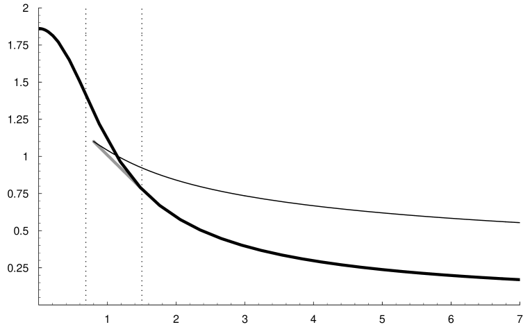
Currently, the best available data for KK phases correspond to six-dimensional KK black holes on $\mathcal{M}^{5}\times S^{1}$ (see e.g.,  Ref. [25] and references therein). We can use the dictionary in appendix F to map the known data to find the curves $a_{H}(\ell)$ for the corresponding phases on $\mathcal{M}^{5}\times\mathbb{T}^{2}$. The resulting phase diagram (based on the numerical results of Ref. [34, 36]) is depicted in Fig. 3. It includes the uniform black membrane, the black membrane with one uniform and one non-uniform direction, and the black string localized in one of the circles of $\mathbb{T}^{2}$. We have also included the $k=2$ copies obtained from these data and the map (8.5). Both the uniform black membrane phase and the localized black string phase extend to $\ell\rightarrow\infty$ where they obey the behavior (8.2) and (8.3) respectively with $n=3$.

Figure 3: $a_{H}(\ell)$ phase diagram in seven dimensions ($\mathcal{M}^{5}\times\mathbb{T}^{2}$) for Kaluza-Klein black hole phases with one uniform direction. Shown are the uniform black membrane phase (dotted), the non-uniform black membrane phase (solid) and the localized black string phase (dashed). For the latter two phases, we have also shown their $k=2$ copy. The non-uniform black membrane phase emanates from the uniform black membrane phase at the GL point $\ell_{\rm GL}=0.811$, while the $k=2$ copy starts at the 2-copied GL point $\ell_{\rm GL}^{(2)}=\sqrt{2}\ell_{\rm GL}=1.15$. The connection between the curves is shown in greater detail. The gap between the solid and dashed curves reflects the difficulty in getting numerical data close to the merger. This figure is representative for the phase diagram of phases on $\mathcal{M}^{D-2}\times\mathbb{T}^{2}$ for all $6\leq D\leq 14$.

The seven-dimensional phase diagram displayed in Fig. 3 is believed to be representative for the black membrane/localized black string phases on $\mathcal{M}^{D-2}\times\mathbb{T}^{2}$ for all $6\leq D\leq 14$. Here the lower bound is obvious since the phase diagram of KK black holes on $\mathcal{M}^{D-2}\times S^{1}$ that we are considering starts at $D=6$. On the other hand, the upper bound follows from the fact that, as explained above, there is a critical dimension $D=14$ above which the behavior of the non-uniform black string phase is qualitatively different [35].

The phase diagram for $D>14$ is much poorly known in comparison, since there are no data like fig. 3 available for the localized and non-uniform phases, only the asymptotic behaviors. We do know, however, that the curve $a_{H}(\ell)$ for non-uniform membranes must again be tangent to the curve of uniform membranes, but now it must lie above the latter, i.e., non-uniform branes have higher entropy than uniform ones. A plausible form of the phase diagram, compatible with the information that we have discussed, is presented in fig. 4. Notice that as $n$ grows larger the asymptotic curves for uniform black membranes and localized black strings, (7.12) and (7.13a), become flatter and closer. In fig. 4 these curves correspond to $D=14$ ($n=10$).

Figure 4: Expected $a_{H}(\ell)$ phase diagram for KK black hole phases with one uniform direction on $\mathcal{M}^{D-2}\times\mathbb{T}^{2}$, when $D>14$. We also show the $k=2$ copy of non-uniform phases, obtained from the main sequence using (8.5). The uniform black membrane curve (dotted) and the asymptotic form of the localized black string curves (dashed) are known exactly. Of the solid lines for non-uniform black membranes, we only know the position of the GL points where they begin, and the fact that they must be tangent to the uniform membrane curve at this point. The points of merger to the black string curves are unknown.

The phases discussed above are the presently known solutions on $\mathcal{M}^{D-2}\times\mathbb{T}^{2}$ that i) have $SO(D-3)$ symmetry; ii) have one uniform direction; and iii) are in thermal equilibrium. If one drops this last condition, there are also multi-localized black string solutions, arising from the multi-black hole configurations on $\mathcal{M}^{D-2}\times S^{1}$ obtained and studied in Ref. [26]. These do also have a counterpart for rotating black holes on $\mathcal{M}^{D}$.

8.3 Phase diagram of neutral rotating black holes on $\mathcal{M}^{D}$

The first observation based on the membrane analogy is that the phase diagram of rotating black holes should also exhibit an infinite sequence of lumpy (pinched) black holes emerging from the curve of MP black holes at increasing values of $j$. This point was made in [31] but let us revisit and elaborate on it a little more here.

It is easy to see, e.g.,  by computing the ratio between the horizon curvatures along the rotation plane and transverse to it, that at large $j$, i.e.,  small $r_{0}/a$, the black membrane is a good approximation to the MP horizon from the rotation axis $\theta=0$ down to values of the polar angle of order

$$\frac{\pi}{2}-\theta\sim\frac{r_{0}}{a}\,.$$ (8.6)

Only very close to the equatorial edge is there a significant deviation from the membrane geometry. For instance, the region $0\leq\theta\mathrel{\raisebox{-2.58334pt}{$\stackrel{{\scriptstyle\textstyle<}}{{\sim}}$}}\frac{\pi}{2}-\frac{r_{0}}{a}$ covers almost all the horizon area, and its length along $\theta$, up to terms of order $r_{0}^{2}/a^{2}$.

Let us now import the GL zero-modes of the black membrane, including the $k$-copies that appear at increasing $\ell$ according to (8.5), into the rotating black hole horizon. We must choose axially-symmetric combinations of the zero modes, so we change basis from plane waves $\exp(ik_{\rm GL}z)$ to Bessel functions. Axially symmetric modes have a profile $J_{0}(k_{\rm GL}a\sin\theta)$ [31]. The basic and simple point here is that the wavenumber, or wavelength $k_{\rm GL}^{-1}$, of the GL zero-mode remains the same in the two analogue systems, to first approximation, even if the profiles are not the same.

At large $j$ the wavelength of GL zero modes, $k_{\rm GL}^{-1}\sim r_{0}$, is much smaller than the extent $\sim a$ along which the horizon looks membrane-like, so we can fit many zeroes of $J_{0}(k_{\rm GL}a\sin\theta)$ in the horizon—this is the analogue of having a high-$k$-copy mode. Over a length $\sim r_{0}$ on the horizon, the relative corrections to the membrane metric due to finite rotation effects are of order [31]

$$\delta g_{\mu\nu}\sim\frac{r_{0}}{a}\;g_{\mu\nu}\,.$$ (8.7)

So the profile of the zero mode will be approximately given by the Bessel function down to polar angles (8.6), and only very near the equator will there appear significant changes. This modifies the boundary conditions along the horizon, relative to those for the black membrane, but by locality, the behavior of modes with much smaller wavelength than the horizon extent will not be significantly modified by edge effects.

As a consequence we can predict the existence of an infinite sequence of pinched black hole phases emanating from the MP curve at increasing values $j_{\rm GL}^{(k)}$. The argument is clearly less strong for the first few GL zero-modes, say, $k=1,2$, where $r_{0}$ and $a$ are comparable so edge effects may become important. The case for the existence of these pinched phases is more strongly made from the need to complete the black ring and black Saturn curves as we shall see below.

We can make one more prediction for the further evolution of the new branches away from the MP curve: like in the membrane case, the Smarr relation and the first law can again be used to prove that two branches of solutions coming out of the same point must be tangent in the $(j,a_{H})$ diagram. However, it is much more difficult to determine which of the branches will have larger area. In particular, the corrections computed in (8.4) enter at order $(r_{0}/L)^{n+4}$. But in the rotating black hole, where we identify $L\sim a$, these are overwhelmed by the finite-rotation corrections (8.7). So (8.4) can not reliably be imported, and in particular the analogy does not allow us to infer the existence of a critical dimension.

Main sequence

The analogy developed above suggests that the phase diagram of rotating black holes in the range $j>j_{\rm mem}$ where MP black holes behave like black membranes, is qualitatively the same as fig. 3, which describes actual membranes and other phases in $\mathcal{M}^{D-2}\times\mathbb{T}^{2}$. Thus we are naturally led to propose that fig. 1 is completed to the phase diagram in Fig. 5. At this moment we are only including the main sequence of non-uniform phases, and not the ‘copied’ phases also present in fig. 3, which will be discussed later.

Figure 5: Qualitative completion of fig. 1 using fig. 3. The gray line corresponds to the conjectured phase of pinched black holes, which branch off tangentially from the MP curve (thick) at a value $j_{\rm GL}>j_{\rm mem}$, and merge with the black ring curve (thin). At any given dimension, the phases may not display the swallowtail in fig. 3, depicted here, but may instead be smoother like fig. 4. Even if there is a cusp, the merger need not happen at it.

Several comments about this diagram are in order. The fact that $a_{H}(j=0)$ is finite for MP black holes while $a_{H}(\ell=0)\to\infty$ for uniform black membranes, is inconsequential since these regions lie at $j<j_{\rm mem}$ where the analogy breaks down. The figure shows the pinched (lumpy) rotating black hole phase as a gray line emerging tangentially from the MP black hole curve at a critical value $j_{\rm GL}$ that is currently unknown. Arguments were given in [31] to the effect that $j_{\rm GL}\mathrel{\raisebox{-2.58334pt}{$\stackrel{{\scriptstyle\textstyle>}}{{\sim}}$}}j_{\rm mem}$, consistently with the analogy. We may have the ‘swallowtail’ structure of first-order phase transitions (as depicted), or instead that of second-order phase transitions, fig. 4. But it may not be unreasonable to expect that a swallowtail appears at least for the lowest dimensions $D=6,7,\dots$, since this is in fact the same type of phase structure that appears for $D=5$.

As we move along the gray line in fig. 5 in the direction away from the MP curve, the pinch at the rotation axis of these black holes grows deeper. Eventually, as depicted in fig. 2, the horizon pinches down to zero thickness at the axis and then the solutions connect to the black ring phase. For all we know, if there is a cusp, the merger need not happen at it.

It would be interesting to study whether the merger happens through a conical geometry, like [53, 54, 55, 38] have argued for non-uniform black string/membrane phases.

Black Saturns and multi-pinch sequences

For KK phases in $\mathcal{M}^{D-2}\times\mathbb{T}^{2}$ there are copies with multiple non-uniformity. However, the implications of these configurations for the phase diagram of rotating black holes on $\mathcal{M}^{D}$ is not straightforward since the analogy becomes less precise for them. The reason is the following. The pinches on a non-uniform membrane are related by a periodic translation symmetry, and so are all exactly equivalent. However, there is no approximate translation symmetry for the pinches on the rotating black hole horizon, even as the ultra-spinning limit is approached. As we have seen, the profiles of the zero-modes, i.e., the pinches at linearized order, are approximately Bessel functions $J_{0}(k_{GL}a\sin\theta)$ away from the equator. Since these functions do not have any discrete translation symmetry along $\theta$, there is actually no limit in which we recover exactly the non-uniform copies for the system on $\mathbb{T}^{2}$. So even if the multiply-pinched phases emerging from the MP curve are, by our arguments above, a natural consequence of the analogy, their development further away from the branch-off point cannot be deduced at all from the analogy.

Nevertheless, even if the correspondence breaks down, we can still argue to infer some qualitative features. Let us proceed by increasing the number of ‘copies’. As we have seen, the most precise application of the analogy to non-uniform phases is to the main sequence (no-copy) phases. For the system on $\mathbb{T}^{2}$ these start from a GL perturbation of the membrane with a single minimum, and then evolve as in fig. 2. Even if the analogue phases (iv) are on one side straight and static, and on the other circular and rotating, their curves (7.14) and (8.3) match up to numerical factors.

Next, the first copy for the non-uniform membrane on $\mathbb{T}^{2}$ begins as a GL zero-mode perturbation of the membrane with two minima, which grows to merge with a configuration of two identical black strings localized on the torus. For the MP black hole, the analogue is the development of a circular pinch, which then grows deeper until the merger with a black Saturn configuration in thermal equilibrium. Thermal equilibrium, i.e.,  equal temperature and angular velocity on all disconnected components of the event horizon, is in fact naturally expected for solutions that merge with pinched black holes, since the temperature and angular velocity of the latter should be uniform on the horizon all the way down to the merger, and we do not expect them to jump discontinuously there. There is no reason to doubt the existence of these black Saturns, but in contrast to the two strings on $\mathbb{T}^{2}$, the two black objects in them are clearly not identical. Still, it is possible to obtain a good approximation for black Saturns in the case when the size of the central black hole is small compared to the radius of the black ring, since then the interaction between the two objects is small and, to a first approximation, one can simply combine them linearly. In five dimensions, where a comparison with exact black Saturn solutions is possible [4], this approximation has been shown to be reliable [5]. It can be readily extended to any $D\geq 5$. One then easily sees that, under the assumption of equal temperatures and angular velocities for the two black objects in the black Saturn, as $j$ is increased a larger fraction of the total mass and the total angular momentum is carried by the black ring, and less by the central black hole. Then, this black Saturn curve must asymptote to the curve of a single black ring.

Strikingly, there is a definite possibility that a second kind of black Saturn, also in thermal equilibrium, exists in $D\geq 6$, which would not have a counterpart in five dimensions. The reason is the following. If we consider MP black holes, and instead of $M$ and $J$ we fix the horizon temperature and angular velocity, then there exist two MP black holes with those values of $T_{H}$ and $\Omega_{H}$: a black hole with a rounded shape, and smaller values of both $M$ and $J$, and another one with larger $M$ and $J$ and a pancaked shape. Now, in our phase diagrams, we fix the total $M$ and $J$ of the black Saturn, but the mass and spin of each of its two constituents are not fixed separately. Instead, under thermal equilibrium we demand that the temperature and angular velocity of the black ring and the central black hole are equal. So besides the black Saturn with a small, round central black hole, that we have discussed above, it may be possible to have another one with a large, pancaked central black hole. These pancaked black Saturns do not have a counterpart in five dimensions, since pancaked black holes with large spin exist only in $D\geq 6$. To get a better idea of the properties of these configurations, we may try to regard them as made of a black ring and a MP black hole that satisfy eqs. (7.1) and (7.5), (7.6), respectively. Then, if the temperatures and angular velocities of the two objects are equal, they must have similar thickness $r_{0}$ and also similar extent along the plane of rotation, $a\sim R$. The latter means that we cannot assume that the two objects are far from each other and interact weakly, and so a simple superposition never becomes really accurate. It is thus conceivable that the black ring can not support itself under the gravitational attraction of the central black hole and so these black Saturns might not actually exist.

Nevertheless, let us assume that they do exist. In this case, even if the approximation based on eqs. (7.1) and (7.5), (7.6) may not be too accurate, it still tells us that most of the mass, angular momentum and area of the black Saturn are concentrated in the central pancaked black hole, while much less of them (by a factor $\sim r_{0}/a$) is in the very thin black ring around it. So the area curve will asymptote (from below) to the curve of a single MP black hole. The two black Saturn curves presumably bifurcate at a value $j\sim O(1)$ near the point of merger with the pinched black hole, but this could happen before, after, or at the merger point. It seems unlikely that the pancaked black Saturn phase appears there and then joins back at larger $j$ to the main-sequence MP curve, since this would appear to require a second merger to a circularly-pinched black hole. Instead, it is more plausible that the pancaked black Saturn continues to exist at larger $j$. In this case, the pancaked central black hole will presumably encounter a GL-like zero-mode from which a new branch of solutions emerges, where the central black hole develops a pinch on the rotation axis—so we will find a pinched black Saturn. We will discuss the possible mergers of this phase after we encounter it again in our subsequent discussion.

The analogy to non-uniform KK phases on $\mathbb{T}^{2}$ becomes even more inadequate when we consider the next ‘copy’, i.e., one more pinch on the rotating black hole horizon. It is certainly expected that at sufficiently large $j$ the rotating MP black hole can fit a zero-mode GL perturbation with both a central pinch and a circular pinch—so a doubly-pinched phase emanates from the curve of smooth MP black holes. However, whereas the pinches on a non-uniform membrane on $\mathbb{T}^{2}$ all evolve, by symmetry, at exactly the same rate, this will not be the case for the corresponding doubly-pinched black hole, where there is no translation symmetry along the polar direction on the horizon. It is therefore unlikely that both pinch down to zero simultaneously. We may expect that the outer, circular pinch, grows deeper faster (in phase space) than the central pinch, since the horizon is thinner away from the axis. In this case, if pinch-down to zero occurs, the pinched black hole will connect not to a black di-ring, but to a black Saturn! This provides, then, a natural way to connect to the pinched black Saturns discussed above. If so, this would prevent the pinch-down to zero of the second, central pinch, and so there would not be any merger to a di-ring. Under these assumptions, there does not appear to be any need, nor in fact much room in the phase diagram, for a black di-ring phase (the ‘analogues’ of the second-copy of localized phases on $\mathbb{T}^{2}$) that, coming from the merger to a single-horizon phase, would be in thermal equilibrium.

In fact the existence, as asymptotic curves at large $j$, of black di-rings, and in general of multi-black rings in thermal equilibrium, already seems difficult for the same reason as in five-dimensions [5]: fixing both the angular velocity and the temperature uniquely determine a black ring, so two black rings in thermal equilibrium with each other have the same radius and would actually be on top of each other. According to this, at least at large values of $j$ multi-rings are unlikely (at smaller $j$ strong gravitational effects might introduce changes). This is nicely consistent with our conclusion above that the ‘second-copy’ pinched black hole does not merge with a di-ring phase but with another phase, presumably a pinched black Saturn. The story repeats, with multiplied complication, for the subsequent multiply-pinched phases.

Summary

Figure 6: Proposal for the phase diagram of thermal equilibrium phases in $D\geq 6$. The solid lines and figures have significant arguments in their favor, while the dashed lines and figures might not exist and admit conceivable, but more complicated, alternatives. Some features have been drawn arbitrarily: at any given bifurcation and in any dimension, smooth connections like fig. 4 are possible instead of swallowtails with cusps; also, the bifurcation into two black Saturn phases may happen before, after, or right at the merger with the pinched black hole. Mergers to di-rings or multi-ring configurations that extend to asymptotically large $j$ seem unlikely. If thermal equilibrium is not imposed, the whole semi-infinite strip $0<a_{H}<a_{H}(j=0)$, $0\leq j<\infty$ is covered, and multi-rings are possible.

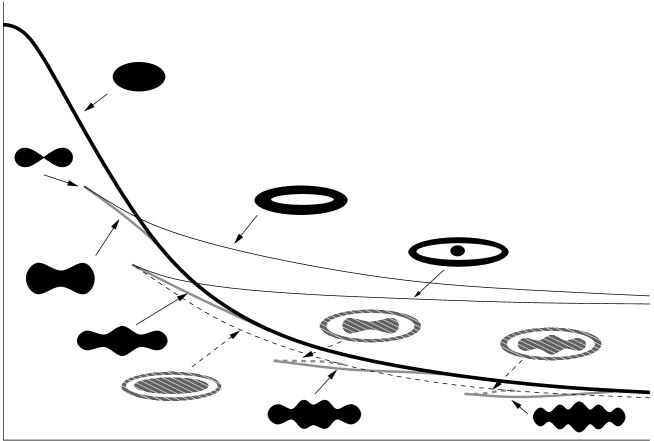
Fig. 6 gives a pictorial description of the phase diagram that we propose. The features that we believe can be argued with confidence (represented with solid lines and figures) are:

1. The black ring phase and its merger to a phase of black holes with a pinch at the rotation axis.

2. The upper black Saturn curve and its merger to a phase of black holes with a circular pinch.

3. An infinite sequence of pinched black hole phases emanating from the MP curve.

4. Any two phases that come out of the same point in the diagram must be tangent at that point. However, for any bifurcation and in any given dimension we cannot predict which of the two phases has higher or lower area near the bifurcation.

The arguments for the second point are as sound as those leading to the first one: the existence of black Saturns can be easily argued when the central black hole is small. The asymptotic value of their area at large $j$ can then be determined and proven to asymptote from below to the black ring value. The merger of these black Saturns to a pinched black hole is then natural.

By constrast, the arguments for pancaked and pinched black Saturns, and the merger of the latter to the pinched black holes that branch off the MP curve, are comparatively less compelling and presumably admit alternatives. Nevertheless, these conjectural phases provide a simple and natural way of completing the curves in the phase diagram that is consistent with all the information available.

We do not expect, at least at asymptotically large $j$, the existence of multi-black rings, with or without a central black hole, in thermal equilibrium. Then, at asymptotically infinite $j$ the only possible phases in thermal equilibrium seem to be MP black holes, black rings, and black Saturns (possibly in two varieties) with a single ring.

We stress that in the diagram of fig. 6 we have represented, of all possible multi-black hole phases, only those that can be in thermal equilibrium, i.e., where the disconnected components of the horizon all have the same temperature and angular velocity. This is natural to impose for phases where disconnected components of the horizon merge to a connected horizon.

In general, however, we expect the existence of multi-black ring configurations, possibly with a central black hole, in which the different black objects have in general different surface gravities and different angular velocities. Although they can not be in thermal equilibrium, they are perfectly valid as stationary multi-black hole configurations of General Relativity—the same remarks as in five dimensions [5] apply to this effect. Since they have additional parameters, they furnish continuous families of solutions filling up a semi-infinite strip of the plane $(j,a_{H})$. At any non-zero $j$, the maximum area is achieved by black Saturns with an almost static central black hole that carries most of the mass, and a very thin and long black ring that carries most of the angular momentum. Imposing thermal equilibrium eliminates the continuous degeneracies and yields solutions characterized by curves $a_{H}(j)$ like in fig. 6.

9 Discussion

The picture we have unveiled for phases of asymptotically flat stationary black holes in higher dimensions is in stark contrast with the four-dimensional phase diagram, which contains only the Kerr solution. The five-dimensional phase diagram for thermal equilibrium phases, fig. 2 in [5], exhibits some similarities to the conjectured phase diagram for thermal equilibrium phases depicted in fig. 6, but there are several significant differences. In five dimensions the merger between the MP and black ring curves occurs at a naked singularity with zero-area, whereas in $D\geq 6$ the pinched-down solution at the merger has finite area and the curvature remains finite on the horizon away from the pinch. It is also amusing to observe that the ‘fat black ring’ branch that is present in $D=5$ is replaced (at least to a large extent) by pinched black holes in $D\geq 6$. This is in accord with the fact that black membranes, uniform or not, do not exist in $D=5$, and with the observation in [43] that fat black rings behave in many respects like ‘drilled-through’ black holes, rather than as circular black strings. More strikingly, while in five dimensions there are only three kinds of single-black hole phases—the MP black hole and the thin and fat black rings—, in $D\geq 6$, following [31], we have been led to include an infinite number of black holes with spherical topology whose horizons have multiple concentric pinches. When they have more than one pinch, their evolution in phase space and their mergers with other thermal equilibrium phases become more speculative. We have also pointed out the possibility of two kinds of thermal-equilibrium black Saturns, only one of which has a five-dimensional counterpart.

So far we have not made almost any mention of the stability of the new solutions, although much of the rich phase structure we have found is actually due to the onset of horizon instabilities. Some instabilities, however, are not expected to give rise to new phases. For instance, black rings at large $j$ in any $D\geq 5$ are expected to suffer from a GL instability that creates ripples along the $S^{1}$ and presumably fragments the black ring into black holes flying apart [2, 39, 43]. It is not known whether this instability switches off or not at $j\sim O(1)$. For large enough $j$, MP and pinched black holes in any dimension might suffer from a similar instability creating ripples along the rotation direction. This instability might radiate away the ‘excess’ angular momentum, or perhaps more likely, break the horizon apart [31]. Additionally, if turning points of $j$ appear in the phase curve (such as the conjectural cusps in fig. 6) then, in analogy to the five-dimensional case [56, 43], we may expect, for the two branches of solutions meeting at the turning point, that the branch with the lowest area will be unstable under radial perturbations to collapse into an MP black hole. Typically, this would apply to pinched black holes, although perhaps not to all of them. If such turning-points for $j$ are absent, pinched black holes will presumably be stable to radial perturbations.

There are several natural extensions of the present work. We discuss some of them here.

A straightforward application of our methods is to study thin black rings in external gravitational potentials. For instance, we may study a thin black ring surrounding a central black hole—thus yielding a black Saturn—, or a black ring in the presence of a cosmological constant—i.e., a black ring in AdS or dS spacetime. The latter may have interesting implications in the AdS/CFT correspondence (see below for additional comments on this). Black rings with charges [58, 59] and with dipoles [60] also satisfy the zero-pressure condition (2.9) and can be analyzed with our methods. These possibilities are currently under investigation.

The general ideas in sec. 2 as well as the specific construction of the linearized solution in sec. 5 can in principle also be extended to analyze black rings with horizon $S^{1}\times S^{n+1}$ with rotation not only along $S^{1}$ but also in the $S^{n+1}$. These involve more functions in the linearized solution, but no new conceptual difficulty is envisaged. The main obstacle is that the near-horizon perturbations of a black string with a rotating $S^{n+1}$ may be quite complicated and perhaps intractable analytically for $n>1$. Nevertheless, we can anticipate that the rotation in the $S^{n+1}$ will introduce particularly rich dynamics for $n\geq 3$, since it is then possible to have ultraspinning regimes for this rotation too. In this case the $S^{n+1}$ can also develop pinches and presumably connect to phases with horizon $S^{1}\times S^{1}\times S^{n}$—and if $n\geq 4$ we can then repeat the story for this last $S^{n}$. For six-dimensional black rings $S^{1}\times S^{3}$, the $S^{3}$ can not pinch, but we may imagine replacing it with a five-dimensional black ring and thus find a horizon $S^{1}\times S^{1}\times S^{2}$.

Clearly, a daunting host of new possibilities opens up as we go higher in $D$. It seems possible to extend the basic, simple core of our ideas in sec. 2, to obtain information about the possible existence of more general blackfolds, obtained by taking a black $p$-brane with horizon topology $\mbox{${\mathbb{R}}^{p}$}\times S^{q}$ and bending ${\mathbb{R}}^{p}$ to form some compact manifold. One must then find out under which conditions a curved black $p$-brane can satisfy the equilibrium equation (2.8). Conventional approaches based on topological considerations have only found very weak restrictions in six or more dimensions [62, 63], and, not being constructive, provide scant information about the actual existence of horizons with other topologies. On the other hand, it is possible to construct time-symmetric initial data containing apparent horizons with the geometry of products of spheres [64], but given the absence of rotation, dynamical evolution should presumably drive these geometries to collapse into a single spherical black hole. Our method, instead, is constructive and uses crucially dynamical information to determine the possible horizon geometries. Notice that several qualitatively new issues must be addressed for $p>1$, since not only the topology, but also the embedding geometry of the worldvolume of a thin black $p$-brane admits much richer possibilities than in the case of a circular ring.

An alternative approach to the matched asymptotic expansion has been developed in [65]. This is a systematic low-energy (long-distance) effective expansion which gives results only in the region away from the black hole and so it does never give directly the corrections to near-horizon magnitudes, only to asymptotic magnitudes. But one can again use Smarr relations and the first law, this time to obtain the corrected area, temperature, and angular velocity. It would be interesting to develop this method to describe extended brane-like black holes such as black strings and possibly other blackfolds.

Another more indirect approach to higher-dimensional black rings in AdS has been put forward recently by Lahiri and Minwalla [66]. In a clever use of the AdS/CFT correspondence they studied stationary, axially symmetric spinning configurations of plasma in ${\cal N}=4$ SYM theory compactified to $d=3$ on a Scherk-Schwarz circle. Such configurations can be studied with the use of the relativistic Navier-Stokes equations, which describe the dynamics of the dual of the horizon, while the radial coordinate away from the horizon is holographically encoded. Thus, one works with equations that depend on one less coordinate than in the gravitational dual, and this makes them more easily tractable. The solutions to these equations correspond to large rotating black holes and black rings in the dual Scherk-Schwarz compactified AdS₅ space. Impressively, the phase diagram of these rotating fluid configurations, even if dual to black holes larger than the AdS radius, reproduces many of the qualitative features of the MP black holes and black rings in five-dimensional flat spacetime. Additional features like the existence of a maximum angular momentum for large black rings presumably reflect the fact that AdS acts like a gravitational well opposing the growth of black rings. Higher-dimensional generalizations of this setup give predictions for the phases of black holes in Scherk-Schwarz compactified AdS_D with $D>5$. Thus, ref. [66] found stationary rotating configurations of fluid that predict rotating black rings in AdS₆ and ‘pinched’ black holes that seem to support, in the AdS context, the conjecture of ‘lumpy’ black holes originally made in [31] and which we have found necessary for completing the higher-dimensional phase diagram. AdS might limit the number of possible pinches and so only a finite number of pinched plasma balls might exist in this context.

The exploration of the possible blackfolds in terms of exact analytic solutions, which has been very successful in four and five dimensions, may turn out to be a hopeless task in higher-dimensional spaces. We hope that the present paper helps to stimulate new approaches to progress further into this fascinating subject.

Appendices

Appendix A Ring-adapted coordinates for flat space

In this appendix we present a useful set of coordinate systems in flat space suitably adapted to a circular ring. We begin by writing the metric of Euclidean flat space ${\mathbb{E}}^{n+3}$ as in (4.2). A hypothetical ring located at $r_{1}=0$ and $r_{2}=R$ is an $S^{1}$ curve embedded in ${\mathbb{E}}^{n+3}$.

Let us consider now a point $\cal P$ located at radii $r_{1}$ and $r_{2}$, angle $\psi=0$ in $S^{1}$ and arbitrary angular location in $S^{n}$. The distance between $\cal P$ and the generic ring point at $r_{1}=0$, $r_{2}=R$ and angle $\psi$ is

$$L(r_{1},r_{2},\psi)=\sqrt{r_{1}^{2}+(R\cos\psi-r_{2})^{2}+R^{2}\sin^{2}\psi}\,.$$ (A.1)

Then $\nabla^{2}\left(L(r_{1},r_{2},\psi)^{-(n+1)}\right)=0$, with a delta-source at the ring point. Integrating over $\psi$ we obtain the total scalar potential at $\cal P$

$$\Sigma(r_{1},r_{2})=\frac{1}{2\pi}\int_{\psi=0}^{2\pi}L(r_{1},r_{2},\psi)^{-(n+1)}\,$$ (A.2)

such that $\nabla^{2}\Sigma=0$ with distributional sources on the ring. To obtain a coordinate system adapted on the equipotential surfaces of $\Sigma$ we define the coordinates $\rho$ and $u$ by

$$\rho^{n+1}=\frac{1}{\Sigma(r_{1},r_{2})}~{},$$ (A.3)

$$\partial_{r_{1}}u=-r_{1}^{n}r_{2}\partial_{r_{2}}\Sigma\ ,\ \ \partial_{r_{2}}u=r_{1}^{n}r_{2}\partial_{r_{1}}\Sigma~{}.$$ (A.4)

The definition of $u$ is such that it is orthogonal to $\rho$, i.e., $g_{\rho u}=0$. In these coordinates the metric is

$$ds^{2}(\mbox{${\mathbb{E}}^{n+3}$})=g_{\rho\rho}d\rho^{2}+g_{uu}du^{2}+r_{1}^{2}d\Omega_{n}^{2}+r_{2}^{2}d\psi^{2}$$ (A.5)

with

$$g_{\rho\rho}=\frac{(n+1)^{2}\Sigma^{\frac{2(n+2)}{n+1}}}{(\partial_{r_{1}}\Sigma)^{2}+(\partial_{r_{2}}\Sigma)^{2}}\ ,\ \ g_{uu}=\frac{1}{r_{1}^{2n}r_{2}^{2}\left[(\partial_{r_{1}}\Sigma)^{2}+(\partial_{r_{2}}\Sigma)^{2}\right]}~{}.$$ (A.6)

For the considerations of the main text it is useful to distinguish between the following regions of spacetime.

The far-zone: $r_{1},r_{2}\gg R$

The leading zeroth order behavior of the potential $\Sigma$ in the asymptotic region $r_{1},r_{2}\gg R$ is

$$\Sigma(r_{1},r_{2})=(r_{1}^{2}+r_{2}^{2})^{-\frac{n+1}{2}}~{}.$$ (A.7)

This implies

$$\rho=\sqrt{r_{1}^{2}+r_{2}^{2}}\ ,\ \ u=\frac{r_{1}^{n+1}}{(r_{1}^{2}+r_{2}^{2})^{\frac{n+1}{2}}}~{}.$$ (A.8)

Defining an angle $\Theta$ such that $u=(\cos\Theta)^{n+1}$ we get

$$r_{1}=\rho\cos\Theta\ ,\ \ r_{2}=\rho\sin\Theta$$ (A.9)

and

$$ds^{2}(\mbox{${\mathbb{E}}^{n+3}$})=d\rho^{2}+\rho^{2}d\Theta^{2}+\rho^{2}\cos^{2}\Theta d\Omega_{n}^{2}+\rho^{2}\sin^{2}\Theta d\psi^{2}~{}.$$ (A.10)

The near-ring-zone: $r_{1}\ll R$ and $|r_{2}-R|\ll R$

In the near-ring region it is more convenient to define a new set of coordinates $r$ and $\theta$ as

$$r(\rho)^{n}=\frac{k_{n}\rho^{n+1}}{R}\ ,\ \ u(\theta)=\mbox{const}+nk_{n}\int_{\theta^{\prime}=0}^{\theta}d\theta^{\prime}(\sin\theta^{\prime})^{n}$$ (A.11)

with

$$k_{n}\equiv\frac{\Omega_{n}}{2\Omega_{n-1}}=\frac{\Gamma(\frac{n}{2})}{2\sqrt{\pi}\Gamma(\frac{n+1}{2})}~{}.$$ (A.12)

To focus locally around the ring we take the limit

$$R\rightarrow\infty\ ,\ \ r_{1}\ \mbox{fixed}\ ,\ \ {\tilde{r}_{2}}=r_{2}-R\ \mbox{fixed}\ ,\ \ z=R\psi\ \mbox{fixed}$$ (A.13)

and expand $\Sigma$ up to first order in $1/R$. Since

$$L^{-(n+1)}=\frac{1}{(r_{1}^{2}+{\tilde{r}_{2}}^{2}+z^{2})^{\frac{n+1}{2}}}-\frac{n+1}{2R}\frac{{\tilde{r}_{2}}z^{2}}{(r_{1}^{2}+{\tilde{r}_{2}}^{2}+z^{2})^{\frac{n+3}{2}}}$$ (A.14)

we deduce that

$$\Sigma=\frac{k_{n}}{R(r_{1}^{2}+{\tilde{r}_{2}}^{2})^{\frac{n}{2}}}\left(1-\frac{{\tilde{r}_{2}}}{2R}\right)~{}.$$ (A.15)

Then

$$r=\sqrt{r_{1}^{2}+{\tilde{r}_{2}}^{2}}\left(1+\frac{{\tilde{r}_{2}}}{2nR}\right)~{},$$ (A.16)

$$u=k_{n+2}\left(\frac{r_{1}}{{\tilde{r}_{2}}}\right)^{n+1}~{}_{2}F_{1}\left(\frac{n+1}{2},\frac{n+2}{2};\frac{n+3}{2};-\frac{r_{1}^{2}}{{\tilde{r}_{2}}^{2}}\right)+\frac{k_{n}}{2R}\frac{r_{1}^{n+1}}{(r_{1}^{2}+{\tilde{r}_{2}}^{2})^{\frac{n}{2}}}~{},$$ (A.17)

$$\cos\theta=\frac{{\tilde{r}_{2}}}{\sqrt{r_{1}^{2}+{\tilde{r}_{2}}^{2}}}\left(1-\frac{1}{2n}\frac{r_{1}^{2}}{{\tilde{r}_{2}}R}\right)~{}.$$ (A.18)

The inverse coordinate transformations are

$$r_{1}=r\sin\theta-\frac{r^{2}}{2nR}\sin 2\theta\,,\qquad r_{2}={\tilde{r}_{2}}+R=R+r\cos\theta-\frac{r^{2}}{2nR}\cos 2\theta~{}.$$ (A.19)

Plugging these expressions into the metric we find the leading $1/R$ form

$$ds^{2}(\mbox{${\mathbb{E}}^{n+3}$})=\left(1+\frac{2r\cos\theta}{R}\right)dz^{2}+\left(1-\frac{2}{n}\frac{r}{R}\cos\theta\right)\left(dr^{2}+r^{2}d\theta^{2}+r^{2}\sin^{2}\theta d\Omega_{n}^{2}\right)~{}.$$ (A.20)

This metric coincides with eq. (5.2), where the adapted coordinates in the near-ring zone were deduced with a more direct approach. The method used here allows us to relate the near-ring coordinates $(r,\theta)$ to the coordinates $(r_{1},r_{2})$ valid everywhere.

Appendix B Relations among the $f_{i}$’s

Given the three sources $T_{tt}$, $T_{t\psi}$, $T_{\psi\psi}$ and the asymptotic boundary conditions, the solution to the linearized Einstein equations is determined, up to gauge transformations, by three independent functions. In (5.5) we introduced six functions $f_{i}$. Here we explain how we can easily derive one of the relations that exists among them.

To find this relation, begin by considering the problem in Cartesian coordinates in the complete, asymptotically flat spacetime (i.e., not just in the overlap zone). We have

$$\nabla^{2}\bar{h}_{tt} = -16\pi GT_{tt}\,,$$ (B.1a)

$$\nabla^{2}\bar{h}_{ti} = -16\pi GT_{ti}\,,$$ (B.1b)

$$\nabla^{2}\bar{h}_{ij} = -16\pi GT_{ij}\,,$$ (B.1c)

where the $T_{ti}$ are obtained from $T_{t\psi}$ and the $T_{ij}$ from $T_{\psi\psi}$ by simply changing coordinates. Now pass from Cartesian to bi-polar coordinates (4.2). Again we will have several non-vanishing components $\bar{h}_{\mu\nu}$. Notice, however, that

$$\bar{h}_{\Omega\Omega}=0\,$$ (B.2)

since it is not sourced by any component of the stress tensor. If we now effect the passage to adapted coordinates (5.2), the components of the metric correction will get mixed in a rather complicated fashion, but (B.2) will still hold. Going over to

$$h_{\mu\nu}=\bar{h}_{\mu\nu}-\frac{1}{n+1}g_{\mu\nu}\bar{h}\,,$$ (B.3)

all components $h_{\mu\nu}$, and hence all the $f_{i}$ in (5.5), will be non-zero, but (B.2) implies,

$$h_{\Omega\Omega}=\frac{1}{2}hg_{\Omega\Omega}\,.$$ (B.4)

This immediately implies (5.6).

Appendix C Regularity of the solutions

In this appendix we examine in detail the implications of regularity for the functions $f_{i}^{(1)}$ that appear in the overlap-zone analysis of sec. 5.2.

The equation for $f_{1}^{(1)}$ and $f_{3}^{(1)}$

The $(tt)$ and $(zz)$ equations in sec. 5.2 take the form (see (5.10)),

$$f^{\prime\prime}+n\cot\theta\,f^{\prime}-(n-1)f=0\,.$$ (C.1)

The change $y=(\sin\theta)^{\frac{n-1}{2}}f$ turns this equation into an associated Legendre equation

$$y^{\prime\prime}+\cot\theta\,y^{\prime}+\left(\ell(\ell+1)-\frac{m^{2}}{\sin^{2}\theta}\right)y=0$$ (C.2)

(often also written after setting $x=\cos\theta$) with indices $\ell=\frac{n-3}{2},\;\frac{1-n}{2}$ and $m=\pm\frac{n-1}{2}$. The two independent solutions can be taken to be the associated Legendre functions of the first and second kind, $P_{\frac{n-3}{2}}^{\frac{1-n}{2}}(\cos\theta)$ and $Q_{\frac{n-3}{2}}^{\frac{n-1}{2}}(\cos\theta)$. So the general solution of (5.10) is

$$f=(\sin\theta)^{\frac{1-n}{2}}\left(c_{1}P_{\frac{n-3}{2}}^{\frac{1-n}{2}}(\cos\theta)+c_{2}Q_{\frac{n-3}{2}}^{\frac{n-1}{2}}(\cos\theta)\right)\,.$$ (C.3)

The prefactor $(\sin\theta)^{\frac{1-n}{2}}$ tends to introduce singularities at $\theta=0,\pi$. The associated Legendre equation has solutions that are non-singular on $\theta\in[0,\pi]$ iff $\ell,m\in\mathbb{Z}$ with $0\leq m\leq\ell$ (or equivalent negative values). So in general the solutions for $f$ are singular at both $\theta=0,\pi$. Non-zero constants $c_{1}$ and $c_{2}$ can be chosen to cancel the singularities at either $\theta=0$ or $\theta=\pi$, but not at both. So regularity requires $c_{1}=c_{2}=0$, i.e.

$$f=0\,.$$ (C.4)

The equation for $f_{6}^{(1)}-f_{5}^{(1)}$

Equation (5.14) is of the form

$$f^{\prime}+(n-1)\cot\theta f-B\sin\theta=0$$ (C.5)

with $f=f_{6}^{(1)}-f_{5}^{(1)}$ and $B=\frac{n+2}{n+1}\tau$. According to (5.16) we must find solutions such that

$$f(0)=f(\pi)=0\,.$$ (C.6)

Defining $w=(\sin\theta)^{n-1}f$, eq. (C.5) becomes

$$w^{\prime}-B(\sin\theta)^{n}=0\,.$$ (C.7)

The general solution of this equation can be written in terms of the hypergeometric function ${}_{2}F_{1}(\alpha,\beta;\gamma;z)$,

$$w=k-B\cos\theta\;_{2}F_{1}\left(\frac{1}{2},\frac{1-n}{2};\frac{3}{2};\cos^{2}\theta\right)\,,$$ (C.8)

with $k$ an integration constant. Eq. (C.6) requires that $w$ vanishes at $\theta=0$ and $\theta=\pi$ faster than $\theta^{n-1}$ and $(\pi-\theta)^{n-1}$, resp. Since $\gamma-\alpha-\beta=\frac{n+1}{2}>0$, the hypergeometric function is finite at $z=\cos^{2}\theta=1$. Actually it takes the same finite value at $\theta=0$ and $\theta=\pi$, but then the factor $\cos\theta$ that multiplies it in (C.8) makes it impossible to choose $k$ so that $w$ vanishes both at $\theta=0$ and $\theta=\pi$. So (C.6) can only be achieved if $B=0$, i.e., if

$$\tau=0\,.$$ (C.9)

Appendix D Solution for ${\sf F}$ and ${\sf G}^{\prime}$

Given the solutions for ${\sf A}$ and ${\sf B}$, eqs. (6.18) with coefficients (6.19) and (6.22), it is straightforward to plug them into (6.2) and (6.14) to obtain ${\sf F}$ and ${\sf G}^{\prime}$. Computing the derivatives using

$$\frac{d}{dz}\;{}_{2}F_{1}(\alpha,\beta;\gamma;z)=\frac{\alpha\beta}{\gamma}\;{}_{2}F_{1}(1+\alpha,1+\beta;1+\gamma;z)$$ (D.1)

and working out the algebra we find

$$\frac{1}{A_{1}}{\sf F} = -r\frac{2n^{2}(n+2)-\left(3n^{3}+4n^{2}+n+4\right)\frac{r_{0}^{n}}{r^{n}}+2(n+2)\frac{r_{0}^{2n}}{r^{2n}}}{n^{2}(n+1)\left(1-\frac{r_{0}^{n}}{r^{n}}\right)\frac{r_{0}^{n}}{r^{n}}}\,_{2}F_{1}\left(-\frac{1}{n},-\frac{n+1}{n};1;1-\frac{r_{0}^{n}}{r^{n}}\right)$$ (D.2)

$$-r\frac{4(3n^{2}+6n+4)-\left(3n(n+3)^{2}+20\right)\frac{r_{0}^{n}}{r^{n}}+4\frac{r_{0}^{2n}}{r^{2n}}}{n^{2}(n+1)^{2}\left(1-\frac{r_{0}^{n}}{r^{n}}\right)}\,_{2}F_{1}\left(-\frac{1}{n},\frac{n-1}{n};1;1-\frac{r_{0}^{n}}{r^{n}}\right)$$

$$-r\frac{2\left(n^{2}-\frac{r_{0}^{n}}{r^{n}}\right)}{n^{3}}\,_{2}F_{1}\left(-\frac{1}{n},\frac{n-1}{n};2;1-\frac{r_{0}^{n}}{r^{n}}\right)$$

$$+\frac{r_{0}^{n}}{r^{n-1}}\frac{2(n-1)\left(3n^{2}+6n+4-\frac{r_{0}^{n}}{r^{n}}\right)}{n^{3}(n+1)^{2}}\,_{2}F_{1}\left(\frac{2n-1}{n},\frac{n-1}{n};2;1-\frac{r_{0}^{n}}{r^{n}}\right)\,,$$

and

$$\frac{1}{A_{1}}{\sf G}^{\prime} = \left(\frac{(n+2)\left(1-2n^{2}\frac{r^{n}}{r_{0}^{n}}\right)}{n^{2}(n+1)}-\frac{2(n-1)}{n^{2}\left(1-\frac{r_{0}^{n}}{r^{n}}\right)}\right)\,_{2}F_{1}\left(-\frac{1}{n},-\frac{n+1}{n};1;1-\frac{r_{0}^{n}}{r^{n}}\right)$$ (D.3)

$$-\frac{4\left(3n^{2}+6n+4\right)-\left(5n^{2}+11n+12\right)\frac{r_{0}^{n}}{r^{n}}+\left(2-n-n^{2}\right)\frac{r_{0}^{2n}}{r^{2n}}}{n^{2}(n+1)^{2}\left(1-\frac{r_{0}^{n}}{r^{n}}\right)}\,_{2}F_{1}\left(-\frac{1}{n},\frac{n-1}{n};1;1-\frac{r_{0}^{n}}{r^{n}}\right)$$

$$-\frac{2n^{2}-(n+2)\frac{r_{0}^{n}}{r^{n}}}{n^{3}}\,_{2}F_{1}\left(-\frac{1}{n},\frac{n-1}{n};2;1-\frac{r_{0}^{n}}{r^{n}}\right)$$

$$+\frac{r_{0}^{n}}{r^{n}}\frac{(n-1)\left(6n^{2}+12n+8-(n+2)\frac{r_{0}^{n}}{r^{n}}\right)}{n^{3}(n+1)^{2}}\,_{2}F_{1}\left(\frac{2n-1}{n},\frac{n-1}{n};2;1-\frac{r_{0}^{n}}{r^{n}}\right)\,.$$

For clarity, we have factored out the overall coefficient $A_{1}$, whose value is given in (6.22a).

Appendix E The five-dimensional black ring solution

Here we recover the known solution for a black ring in five dimensions [2, 3], in the limit of small $r_{0}/R$, using the methods developed in this paper. This is of interest not only as a check of our approach, but also because there is one significant difference with respect to the higher-dimensional ($n>1$) cases that merits special attention. It implies the existence of corrections to the physical magnitudes $\mathcal{A}$, $M$, $J$, $\kappa$, $\Omega$ at order $1/R$.

E.1 The linearized solution in ‘ring coordinates’ $(x,y)$

The five-dimensional black ring is most often written using a set of adapted coordinates $(x,y)$, in which five-dimensional Minkowski space is

$$g^{0}_{\mu\nu}dx^{\mu}dx^{\nu}=-dt^{2}+\frac{R^{2}}{(x-y)^{2}}\left[\frac{dy^{2}}{y^{2}-1}+(y^{2}-1)d\psi^{2}+\frac{dx^{2}}{1-x^{2}}+(1-x^{2})d\phi^{2}\right]\,.$$ (E.1)

See [3] for an explanation of this coordinate system. Here $-R/y$ plays the role of a radial coordinate and $\arccos(x)$ is a polar angle, but constant $y$ and constant $x$ do not coincide with constant $r$ and $\theta$ as we have defined them in this paper.

We solve the linear Einstein equations with $T_{\mu\nu}$ given by

$$T_{tt}=\frac{M}{2\pi R}\delta(-R/y)\,,\qquad T_{t\psi}=\frac{J}{2\pi R}\delta(-R/y)\,.$$ (E.2)

The ring lies at $y\to-\infty$. The linearized Einstein equations in transverse gauge (4.1) are very easy to solve for the sources (E.2). The $tt$ equation is the Laplace equation with sources on a ring, whose solution is

$$\bar{h}_{tt}=\frac{2GM}{\pi R^{2}}(x-y)$$ (E.3)

while the $t\psi$ equation is the same as we get for the $B_{t\psi}$ field of a ring of string [3],

$$\bar{h}_{t\psi}=-\frac{2GJ}{\pi R^{2}}(1+y)\,.$$ (E.4)

Then $h_{\mu\nu}=\bar{h}_{\mu\nu}-\frac{1}{3}\bar{h}g_{\mu\nu}$ is

$$h_{tt}=\frac{4GM}{3\pi R^{2}}(x-y)\,,\quad h_{t\psi}=-\frac{2GJ}{\pi R^{2}}(1+y)\,,\quad h_{ij}=g_{ij}\frac{2GM}{3\pi R^{2}}(x-y)$$ (E.5)

In principle, here $M$ and $J$ are independent quantities since their respective sources enter separately the linearized equations, but we know they must be related. We introduce a dimensionless parameter

$$\nu=\frac{2GM}{3\pi R^{2}}=\frac{\sqrt{2}GJ}{\pi R^{3}}$$ (E.6)

so

$$h_{tt}=2\nu(x-y)\,,\quad h_{t\psi}=-\sqrt{2}\nu R(1+y)\,,\quad h_{ij}=\nu(x-y)g_{ij}^{0}$$ (E.7)

This solution is not in the same gauge as in [60, 3]. To go to the latter, change coordinates

$$x=\hat{x}-\frac{\nu}{2}(\hat{x}^{2}-1)\,,\qquad y=\hat{y}-\frac{\nu}{2}(\hat{y}^{2}-1)$$ (E.8)

so that

$$g_{xx}dx^{2}=(1+\nu\hat{y})\hat{g}_{\hat{x}\hat{x}}d\hat{x}^{2}\,,\qquad g_{\phi\phi}=(1+\nu\hat{y})\hat{g}_{\phi\phi}$$ (E.9)

and correspondingly for $x\leftrightarrow y$, $\phi\to\psi$. The new solution, dropping hats, is

$$h_{tt}=2\nu(x-y)\,,\quad h_{t\psi}=-\sqrt{2}\nu R(1+y)\,,$$ (E.10a)

$$h_{\psi\psi}=(\nu x+\nu(x-y))g^{0}_{\psi\psi}\,,\quad h_{\phi\phi}=(\nu y+\nu(x-y))g^{0}_{\phi\phi}\,,$$ (E.10b)

$$h_{xx}=(\nu y+\nu(x-y))g^{0}_{xx}\,,\quad h_{yy}=(\nu x+\nu(x-y))g^{0}_{yy}\,.$$ (E.10c)

This reproduces the solution in [60, 3] to linear order in $\nu$.

E.2 The solution in $(r_{1},r_{2})$ and $(r,\theta)$ coordinates: the issue of $1/R$ corrections

The previous calculation showed how the known solution is recovered to linearized approximation around flat space. However, a puzzling fact emerges when one notices that the expressions for $\mathcal{A}$, $M$, and $J$ in the exact solution, when expanded in $\nu=r_{0}/R$, receive corrections at linear order. This would seem to contradict our general argument in section 6 that, since the perturbations to the boosted black string are of dipole type, there should not be any corrections. The resolution is instructive.

The integrals (4.4), (4.5) for the linearized potentials can be calculated explicitly (see [44]),

$$\Phi = \frac{4GM}{3\pi}\frac{1}{\sqrt{\left(r_{1}^{2}+r_{2}^{2}+R^{2}\right)^{2}-4r_{2}^{2}R^{2}}}\,,$$ (E.11a)

$$A = \frac{2GJ}{\pi R^{2}}\left(\frac{r_{1}^{2}+r_{2}^{2}+R^{2}}{\sqrt{\left(r_{1}^{2}+r_{2}^{2}+R^{2}\right)^{2}-4r_{2}^{2}R^{2}}}-1\right)\,.$$ (E.11b)

The relation between the coordinates $(r_{1},r_{2})$ and $(x,y)$ used in the previous section, can be found in [3]. It is then straightforward to check that (E.11) yield the same solution (in transverse gauge) as the linearized solution of the previous section. This solution can be expanded now in the overlap zone $r_{0}\ll r\ll R$, using the change of coordinates (A.19) and the relation (2.11) between parameters. We find

$$\Phi = \frac{r_{0}}{r}\left(1+O\left(\frac{r_{0}}{r}\right)+O\left(\frac{r^{2}}{R^{2}}\right)\right)\,,$$ (E.12)

$$A = R\frac{\sqrt{2}r_{0}}{r}\left(1+\frac{r(\cos\theta-1)}{R}+O\left(\frac{r_{0}}{r}\right)+O\left(\frac{r^{2}}{R^{2}}\right)\right)\,.$$ (E.13)

Then, to the appropriate order in the overlap zone,

$$g_{tt} = -1+\frac{2r_{0}}{r}\,,$$ (E.14a)

$$g_{tz} = -\frac{\sqrt{2}r_{0}}{r}\left(1+\frac{r(\cos\theta-1)}{R}\right)\,,$$ (E.14b)

$$g_{zz}=1+\frac{r_{0}}{r}\left(1+\frac{2r}{R}\cos\theta\right)+\frac{2r}{R}\cos\theta\,,$$ (E.14c)

$$g_{rr}=1+\frac{r_{0}}{r}\left(1-\frac{2r\cos\theta}{R}\right)-\frac{2r\cos\theta}{R}\,,$$ (E.14d)

$$g_{\theta\theta}=r^{2}\left[1+\frac{r_{0}}{r}\left(1-\frac{2r\cos\theta}{R}\right)-\frac{2r\cos\theta}{R}\right]\,,$$ (E.14e)

$$g_{\phi\phi}=r^{2}\sin^{2}\theta\left[1+\frac{r_{0}}{r}\left(1-\frac{2r\cos\theta}{R}\right)-\frac{2r\cos\theta}{R}\right]\,.$$ (E.14f)

This solution must now be compared to the one we obtained, also in transverse gauge, in section 5, eqs. (5.21) with $n=1$, where we solved the equations directly in the overlap zone. That solution, in fact, provided the basis for our claim that only perturbations of dipole type affect the near-horizon geometry. Hence, the origin of the discrepancy must be visible there. Indeed, comparing the solutions we find that all terms in (5.21) with $n=1$ agree with (E.14) except for $g_{tz}$: in (E.14b) there is a term $\propto r_{0}/R$ of monopole type, i.e., independent of $\theta$, which is absent in (5.21b).

The difference between (5.21b) and (E.14b) is pure gauge, since we can obtain the latter from the former by making

$$t\to t-\frac{\sqrt{2}\,r_{0}}{R}z\,,$$ (E.15)

which is indeed a gauge transformation involving a monopole term. However, this does not mean that the difference is physically irrelevant. The discrepant monopole term at order $1/R$ shows up as a constant in $A$ in (E.12), and so it can be traced back to the choice of integration constant in (E.11). This was chosen to make $A$ vanish at the $\psi$-rotation axis $r_{2}=0$, as is required for the one-form $Ad\psi$ to be well-defined. So this condition removes the freedom to change $t\to t+k\psi=t+\frac{k}{R}z$, although this is not evident when working in the overlap zone. In other words, regularity at the rotation axis demands that we change (5.21b) (for $n=1$) to the regular gauge (E.15). As a consequence, the monopole perturbation in (E.14b), even if gauge, is physical. This is an example of how a gauge degree of freedom becomes physical due to boundary conditions.

Since this perturbation changes the monopolar part of the solution, it induces corrections of order $1/R$ in the physical magnitudes $\mathcal{A}$, $M$, $J$, $\kappa$, $\Omega$, with the correct values to reproduce the exact results to linear order in $r_{0}/R$. Such an effect, however, is absent in six or more dimensions, where the field $A$ falls faster away from the source.

E.3 The near-horizon solution

The analysis in sec. 6 simplifies considerably in the case $n=1$ and allows us to be fully explicit, since

$$u_{1}=3r-2r_{0}\,,\qquad u_{2}=r_{0}\,,$$ (E.16)

and $A_{1}=-4/3$, $A_{2}=-14/3$, $B_{1}=-2/3$, $B_{2}=-4/3$. Then

$${\sf A}(r)=-4r-2r_{0}\,,\qquad{\sf B}(r)=-2r\,,$$ (E.17)

and

$${\sf F}(r)=4r+4r_{0}+\frac{12r^{2}}{r_{0}}-\frac{4r^{2}}{r-r_{0}}\,,\qquad{\sf G}^{\prime}(r)=-2+\frac{8r}{r-r_{0}}+\frac{12r}{r_{0}}\,.$$ (E.18)

So

$$a(r)=-4r-2r_{0}+2c(r)\,,\qquad b(r)=-2r+c(r)\,,$$ (E.19)

and

$$f(r) = 4r+4r_{0}+\frac{12r^{2}}{r_{0}}-\frac{4r^{2}}{r-r_{0}}+\frac{rc(r)}{r-r_{0}}-\frac{4r}{r_{0}}c(r)-\frac{2r^{2}}{r_{0}}c^{\prime}(r)\,,$$ (E.20a)

$$g^{\prime}(r) = -2+\frac{8r}{r-r_{0}}+\frac{12r}{r_{0}}-\frac{2c(r)}{r-r_{0}}-\frac{4c(r)}{r_{0}}-\frac{2r}{r_{0}}c^{\prime}(r)\,.$$ (E.20b)

Boundary conditions at the horizon and at large $r$ require that the function $c(r)$ takes the form

$$c(r)=2r+r_{0}+\frac{r_{0}^{2}}{r}+\frac{r_{0}^{3}}{r^{2}}\,\tilde{c}(r)\,,$$ (E.21)

where the gauge-dependent function $\tilde{c}(r)$ is an analytic function of $1/r$ with $\tilde{c}(r_{0})=0$. The value $c(r_{0})=4r_{0}$ guarantees that $f$ and $g^{\prime}$ are regular at $r=r_{0}$ in spite of the fact that ${\sf F}$ and ${\sf G}^{\prime}$ are singular there.

In order to make a choice of gauge, let us impose $g(r)=f(r)$. Then (E.20) require that $\tilde{c}$ solves

$$2r^{2}(r-r_{0})^{2}\tilde{c}^{\prime\prime}(r)-r(r-r_{0})(2r-r_{0})\tilde{c}^{\prime}(r)+r_{0}^{2}\;\tilde{c}(r)=0\,,$$ (E.22)

which can be transformed into an associated Legendre equation. The only solution with the prescribed behavior at the boundaries is

$$\tilde{c}(r)=0\,.$$ (E.23)

Then

$$f(r)=g(r)=-2r+r_{0}\,.$$ (E.24)

The solution in [2], to leading order in $r_{0}/R$, is in fact in this gauge.

Finally, in order to illustrate the fact that the distortion of the $S^{2}$ at the horizon, $g(r_{0})$, is gauge-dependent and so can take any arbitrary value (at least to leading order in $1/R$), choose instead

$$\tilde{c}(r)=c_{1}\left(1-\frac{r_{0}}{r}\right)$$ (E.25)

with constant $c_{1}$ (of course this makes $f\neq g$ in general). $g^{\prime}$ is easily integrated, and the asymptotic behavior $g(r)+2r\to 0$ at $r\to\infty$ fixes the integration constant. Then we find that $g(r_{0})=(2c_{1}-1)r_{0}$. So the sign of the distortion of the $S^{2}$ at the horizon is arbitrary, and it can even remain perfectly round.

Appendix F KK phases on $\mathbb{T}^{2}$ from phases on $S^{1}$

In this appendix we show how to translate the known results for KK black holes on the circle (${\it i.e.,\,}$ on $\mathcal{M}^{n+2}\times S^{1}$) to the corresponding results for KK black holes on the torus (${\it i.e.,\,}$ on $\mathcal{M}^{n+2}\times\mathbb{T}^{2}$), which are used in section 8.

New dimensionless quantities

We first recall that for KK black holes in $D$ dimensions, the typical dimensionless quantities that are used are the dimensionless mass $\mu$, temperature $\mathfrak{t}$, and entropy $\mathfrak{s}$ defined by

$$\mu=\frac{16\pi G}{L^{D-3}}\;M\ ,\ \ \mathfrak{s}=\frac{16\pi G}{L^{D-2}}\;S\ ,\ \ \mathfrak{t}=LT\ .$$ (F.1)

These quantities were originally introduced in [67, 68] for black holes on a KK circle of circumference $L$, but we may similarly use these definitions for KK black holes in $D$ dimensions with a square torus of side lengths $L$.

Instead of these, we now introduce the following new dimensionless quantities, more suitable for the application in this paper, by defining

$$\ell=\mu^{-\frac{1}{D-3}}\ ,\ \ a_{H}=\mu^{-\frac{D-2}{D-3}}\mathfrak{s}\ ,\ \ \mathfrak{t}_{H}=\mu^{\frac{1}{D-3}}\mathfrak{t}\,.$$ (F.2)

In the KK black hole literature, entropy plots are typically given as $\mathfrak{s}(\mu)$. Instead of these we then use (F.2) to consider the area function $a_{H}(\ell)$, which is obtained as

$$a_{H}(\ell)=\ell^{D-2}\mathfrak{s}(\ell^{-D+3})\,.$$ (F.3)

Map from circle to torus compactification

In the following we use hatted quantities to refer to KK black holes on $\mathcal{M}^{n+1}\times S^{1}$ and unhatted quantities when referring to KK black holes on $\mathcal{M}^{n+2}\times\mathbb{T}^{2}$. Note that in the latter case the definitions (F.2) for $\ell$, $a_{H}$ reduce to those in (8.1), and that the definition of $\mathfrak{t}_{H}$ is up to constants identical to the one in (7.8b).

Suppose we are given an entropy function $\hat{\mathfrak{s}}(\hat{\mu})$ for a phase of KK black holes on $\mathcal{M}^{n+2}\times S^{1}$. Any such phase lifts trivially to a phase of KK black holes on $\mathcal{M}^{n+2}\times\mathbb{T}^{2}$ that is uniform in one of the torus directions. We want to know how we get the function $a_{H}(l)$ for the latter in terms of $\hat{\mathfrak{s}}(\hat{\mu})$ of the former. It is not difficult to see that in terms of our original dimensionless quantities we have the simple mapping

$$\mu=\hat{\mu}\ ,\ \ \mathfrak{s}=\hat{\mathfrak{s}}\ ,\ \ \mathfrak{t}=\hat{\mathfrak{t}}\,.$$ (F.4)

It then follows from (F.2) and (F.3) that the area function $a_{H}(\ell)$ of KK black holes on $\mathcal{M}^{n+2}\times\mathbb{T}^{2}$ is obtained via the mapping relation

$$a_{H}(\ell)=\ell^{n+2}\hat{\mathfrak{s}}(\ell^{-n-1})\,.$$ (F.5)

Application to known phases

Using now the entropy function of the uniform black string in $\mathcal{M}^{n+2}\times S^{1}$

$$\hat{\mathfrak{s}}_{\rm uni}(\hat{\mu})\sim\hat{\mu}^{\frac{n}{n-1}}$$ (F.6)

we get from (F.5) the result (8.2) for $a_{H}^{\rm ubm}(\ell)$ of the uniform black membrane. Furthermore, using that for small $\mu$ (or equivalently large $\ell$) the entropy of the localized black hole in $\mathcal{M}^{n+2}\times S^{1}$ is

$$\hat{\mathfrak{s}}_{\rm loc}(\hat{\mu})\sim\hat{\mu}^{\frac{n+1}{n}}$$ (F.7)

we find via the map (F.5) the result (8.3) for $a_{H}^{\rm lbs}(\ell)$ of the localized black string in the large $\ell$ limit.

For the non-uniform string in $\mathcal{M}^{n+2}\times S^{1}$ dimensions we know that (see e.g. Eq.(3.16) in [25])

$$\frac{\hat{\mathfrak{s}}_{\rm nu}(\hat{\mu})}{\hat{\mathfrak{s}}_{\rm uni}(\hat{\mu})}=1-\frac{n^{2}}{2(n+1)(n-1)^{2}}\frac{\gamma_{n+2}}{\hat{\mu}_{{\rm GL},n+2}}(\hat{\mu}-\hat{\mu}_{{\rm GL},n+2})^{2}+\mathcal{O}((\hat{\mu}-\hat{\mu}_{{\rm GL},n+2})^{3})\ ,$$ (F.8)

where $\hat{\mathfrak{s}}_{\rm uni}(\hat{\mu})$ is the entropy of the uniform black string and $\hat{\mu}_{{\rm GL},d}$, $\gamma_{d}$ can e.g. be found in Tables 2,3 of the review [25]. The result (8.4) for the black membrane on $\mathcal{M}^{n+2}\times\mathbb{T}^{2}$ with non-uniformity in one direction then follows again using (F.8) and the map (F.5).

It is also known that the localized black hole and non-uniform black string phase on $\mathcal{M}^{n+2}\times S^{1}$ have ’copied’ phases with multiple non-uniformity or multiple localized black objects [51, 52]. In particular, the copies (denoted with a tilde) are obtained from the original phases using

$$\tilde{\hat{\mu}}=\frac{\hat{\mu}}{k^{n-1}}\ ,\ \ \tilde{\hat{\mathfrak{s}}}=\frac{\hat{\mathfrak{s}}}{k^{n}}\ ,\ \ \tilde{\hat{\mathfrak{t}}}=k\hat{\mathfrak{t}}\ ,$$ (F.9)

where $k$ is a positive integer denoting how many times the solution is copied. Using the relation (F.4) and the definitions (F.2) then shows that the corresponding copied phases of KK black holes on the torus obey the transformation rule (8.5).

Finally, we give the explicit mapping used to convert the known results for KK black holes on $\mathcal{M}^{5}\times S^{1}$ to obtain the phase diagram in Fig. 3 of KK black holes on $\mathcal{M}^{5}\times\mathbb{T}^{2}$. We start with the six-dimensional numerical data that are known for the non-uniform and localized phase [36], which have been converted to plots of points $(\hat{\mu},\hat{\mathfrak{s}})$ (see e.g. [25]). Using (F.4), (F.2) these data are then easily transformed to curves in an $a_{H}(\ell)$ phase diagram for phases in seven dimensions with a torus, according to

$$(\ell,a_{H})=(\hat{\mu}^{-1/4},\hat{\mu}^{-5/4}\hat{\mathfrak{s}})\,.$$ (F.10)

References

- [1] R. C. Myers and M. J. Perry, “Black holes in higher dimensional space-times,” Ann. Phys. 172 (1986) 304.
- [2] R. Emparan and H. S. Reall, “A rotating black ring in five dimensions,” Phys. Rev. Lett. 88 (2002) 101101, hep-th/0110260.
- [3] R. Emparan and H. S. Reall, “Black rings,” Class. Quant. Grav. 23 (2006) R169, hep-th/0608012.
- [4] H. Elvang and P. Figueras, “Black saturn,” JHEP 05 (2007) 050, hep-th/0701035.
- [5] H. Elvang, R. Emparan, and P. Figueras, “Phases of five-dimensional black holes,” JHEP 05 (2007) 056, hep-th/0702111.
- [6] H. Iguchi and T. Mishima, “Black di-ring and infinite nonuniqueness,” Phys. Rev. D75 (2007) 064018, hep-th/0701043.
- [7] J. Evslin and C. Krishnan, “The black di-ring: An inverse scattering construction,” arXiv:0706.1231 [hep-th].
- [8] V. A. Belinsky and V. E. Zakharov, “Integration of the Einstein equations by the inverse scattering problem technique and the calculation of the exact soliton solutions,” Sov. Phys. JETP 48 (1978) 985–994.
- [9] V. A. Belinsky and V. E. Zakharov, “Stationary gravitational solitons with axial symmetry,” Sov. Phys. JETP 50 (1979) 1.
- [10] V. Belinski and E. Verdaguer, “Gravitational solitons,”. Cambridge, UK: Univ. Pr. (2001) 258 p.
- [11] A. A. Pomeransky, “Complete integrability of higher-dimensional Einstein equations with additional symmetry, and rotating black holes,” Phys. Rev. D73 (2006) 044004, hep-th/0507250.
- [12] A. A. Pomeransky and R. A. Sen’kov, “Black ring with two angular momenta,” hep-th/0612005.
- [13] H. Elvang and M. J. Rodríguez, “Bicycling black rings,”.
- [14] P.-J. De Smet, “On stationary metrics in five dimensions,” gr-qc/0306026.
- [15] A. Coley, R. Milson, V. Pravda, and A. Pravdova, “Classification of the Weyl tensor in higher-dimensions,” Class. Quant. Grav. 21 (2004) L35–L42, gr-qc/0401008.
- [16] A. Coley and N. Pelavas, “Classification of higher dimensional spacetimes,” Gen. Rel. Grav. 38 (2006) 445–461, gr-qc/0510064.
- [17] V. Pravda, “On the algebraic classification of spacetimes,” J. Phys. Conf. Ser. 33 (2006) 463–468, gr-qc/0512087.
- [18] Y. Morisawa and D. Ida, “A boundary value problem for the five-dimensional stationary rotating black holes,” Phys. Rev. D69 (2004) 124005, gr-qc/0401100.
- [19] S. Hollands and S. Yazadjiev, “Uniqueness theorem for 5-dimensional black holes with two axial killing fields,” arXiv:0707.2775 [gr-qc].
- [20] T. Harmark, “Stationary and axisymmetric solutions of higher-dimensional general relativity,” Phys. Rev. D70 (2004) 124002, hep-th/0408141.
- [21] T. Harmark and P. Olesen, “On the structure of stationary and axisymmetric metrics,” Phys. Rev. D72 (2005) 124017, hep-th/0508208.
- [22] R. Emparan and H. S. Reall, “Generalized Weyl solutions,” Phys. Rev. D65 (2002) 084025, hep-th/0110258.
- [23] S. Giusto and A. Saxena, “Stationary axisymmetric solutions of five dimensional gravity,” arXiv:0705.4484 [hep-th].
- [24] B. Kol, “The phase transition between caged black holes and black strings: A review,” Phys. Rept. 422 (2006) 119–165, hep-th/0411240.
- [25] T. Harmark, V. Niarchos, and N. A. Obers, “Instabilities of black strings and branes,” Class. Quant. Grav. 24 (2007) R1–R90, hep-th/0701022.
- [26] O. J. C. Dias, T. Harmark, R. C. Myers, and N. A. Obers, “Multi-black hole configurations on the cylinder,” arXiv:0706.3645 [hep-th].
- [27] T. Harmark, “Small black holes on cylinders,” Phys. Rev. D69 (2004) 104015, hep-th/0310259.
- [28] D. Gorbonos and B. Kol, “A dialogue of multipoles: Matched asymptotic expansion for caged black holes,” JHEP 06 (2004) 053, hep-th/0406002.
- [29] D. Karasik, C. Sahabandu, P. Suranyi, and L. C. R. Wijewardhana, “Analytic approximation to 5 dimensional black holes with one compact dimension,” Phys. Rev. D71 (2005) 024024, hep-th/0410078.
- [30] D. Gorbonos and B. Kol, “Matched asymptotic expansion for caged black holes: Regularization of the post-Newtonian order,” Class. Quant. Grav. 22 (2005) 3935–3960, hep-th/0505009.
- [31] R. Emparan and R. C. Myers, “Instability of ultra-spinning black holes,” JHEP 09 (2003) 025, hep-th/0308056.
- [32] R. Gregory and R. Laflamme, “Black strings and -branes are unstable,” Phys. Rev. Lett. 70 (1993) 2837–2840, hep-th/9301052.
- [33] S. S. Gubser, “On non-uniform black branes,” Class. Quant. Grav. 19 (2002) 4825–4844, hep-th/0110193.
- [34] T. Wiseman, “Static axisymmetric vacuum solutions and non-uniform black strings,” Class. Quant. Grav. 20 (2003) 1137–1176, hep-th/0209051.
- [35] E. Sorkin, “A critical dimension in the black-string phase transition,” Phys. Rev. Lett. 93 (2004) 031601, hep-th/0402216.
- [36] H. Kudoh and T. Wiseman, “Connecting black holes and black strings,” Phys. Rev. Lett. 94 (2005) 161102, hep-th/0409111.
- [37] B. Kleihaus, J. Kunz, and E. Radu, “New nonuniform black string solutions,” JHEP 06 (2006) 016, hep-th/0603119.
- [38] E. Sorkin, “Non-uniform black strings in various dimensions,” Phys. Rev. D74 (2006) 104027, gr-qc/0608115.
- [39] J. L. Hovdebo and R. C. Myers, “Black rings, boosted strings and Gregory-Laflamme,” Phys. Rev. D73 (2006) 084013, hep-th/0601079.
- [40] D. Kastor, S. Ray, and J. Traschen, “The first law for boosted Kaluza–Klein black holes,” JHEP 06 (2007) 026, arXiv:0704.0729 [hep-th].
- [41] B. Carter, “Essentials of classical brane dynamics,” Int. J. Theor. Phys. 40 (2001) 2099–2130, gr-qc/0012036.
- [42] H. Elvang and R. Emparan, “Black rings, supertubes, and a stringy resolution of black hole non-uniqueness,” JHEP 11 (2003) 035, hep-th/0310008.
- [43] H. Elvang, R. Emparan, and A. Virmani, “Dynamics and stability of black rings,” JHEP 12 (2006) 074, hep-th/0608076.
- [44] R. Emparan, D. Mateos, and P. K. Townsend, “Supergravity supertubes,” JHEP 07 (2001) 011, hep-th/0106012.
- [45] O. Lunin, J. M. Maldacena, and L. Maoz, “Gravity solutions for the D1-D5 system with angular momentum,” hep-th/0212210.
- [46] T. Harmark and N. A. Obers, “Black holes on cylinders,” JHEP 05 (2002) 032, hep-th/0204047.
- [47] B. Kol, “The power of action: ’The’ derivation of the black hole negative mode,” hep-th/0608001.
- [48] B. Kol, “Perturbations around backgrounds with one non-homogeneous dimension,” hep-th/0609001.
- [49] I. Racz and R. M. Wald, “Extension of space-times with Killing horizon,” Class. Quant. Grav. 9 (1992) 2643–2656.
- [50] R. Gregory and R. Laflamme, “Hypercylindrical black holes,” Phys. Rev. D37 (1988) 305.
- [51] G. T. Horowitz, “Playing with black strings,” hep-th/0205069.
- [52] T. Harmark and N. A. Obers, “Phase structure of black holes and strings on cylinders,” Nucl. Phys. B684 (2004) 183–208, hep-th/0309230.
- [53] B. Kol, “Topology change in general relativity and the black-hole black-string transition,” hep-th/0206220.
- [54] T. Wiseman, “From black strings to black holes,” Class. Quant. Grav. 20 (2003) 1177–1186, hep-th/0211028.
- [55] B. Kol and T. Wiseman, “Evidence that highly non-uniform black strings have a conical waist,” Class. Quant. Grav. 20 (2003) 3493–3504, hep-th/0304070.
- [56] G. Arcioni and E. Lozano-Tellechea, “Stability and critical phenomena of black holes and black rings,” Phys. Rev. D72 (2005) 104021, hep-th/0412118.
- [57] H. K. Kunduri, J. Lucietti, and H. S. Reall, “Do supersymmetric anti-de Sitter black rings exist?,” JHEP 02 (2007) 026, hep-th/0611351.
- [58] H. Elvang, “A charged rotating black ring,” hep-th/0305247.
- [59] H. Elvang, R. Emparan, D. Mateos, and H. S. Reall, “A supersymmetric black ring,” Phys. Rev. Lett. 93 (2004) 211302, hep-th/0407065.
- [60] R. Emparan, “Rotating circular strings, and infinite non-uniqueness of black rings,” JHEP 03 (2004) 064, hep-th/0402149.
- [61] A. Dabholkar, N. Iizuka, A. Iqubal, A. Sen and M. Shigemori, “Spinning strings as small black rings,” JHEP 0704 (2007) 017 [arXiv:hep-th/0611166].
- [62] C. Helfgott, Y. Oz, and Y. Yanay, “On the topology of black hole event horizons in higher dimensions,” JHEP 02 (2006) 025, hep-th/0509013.
- [63] G. J. Galloway and R. Schoen, “A generalization of Hawking’s black hole topology theorem to higher dimensions,” Commun. Math. Phys. 266 (2006) 571–576, gr-qc/0509107.
- [64] F. Schwartz, “Existence of outermost apparent horizons with product of spheres topology,” arXiv:0704.2403 [gr-qc].
- [65] Y.-Z. Chu, W. D. Goldberger, and I. Z. Rothstein, “Asymptotics of -dimensional Kaluza-Klein black holes: Beyond the Newtonian approximation,” JHEP 03 (2006) 013, hep-th/0602016.
- [66] S. Lahiri and S. Minwalla, “Plasmarings as dual black rings,” arXiv:0705.3404 [hep-th].
- [67] T. Harmark and N. A. Obers, “New phase diagram for black holes and strings on cylinders,” Class. Quantum Grav. 21 (2004) 1709–1724, hep-th/0309116.
- [68] T. Harmark and N. A. Obers, “New phases of near-extremal branes on a circle,” JHEP 09 (2004) 022, hep-th/0407094.