Associated production of graviton with $e^{+}e^{-}$ pair via photon-photon collisions at a linear collider

Abstract

We investigate the process $\gamma\gamma\to e^{+}e^{-}G_{n}~{}$at the future International Linear Collider(ILC), where $G_{n}$ is the Kaluza-Klein graviton in the Large Extra Dimension Model. When the fundamental energy scale is of a few ${\rm TeV}$, the cross section of this process can reach several hundred $fb$ at a photon-photon collider with $\sqrt{s}=500\sim 1000~{}GeV$, and the cross section in J=2 polarized photon collision mode is much larger than that in J=0 polarized photon collision mode. We present strategies to distinguish the graviton signal from numerous $SM$ backgrounds, and find that the graviton signal with extra dimensions $\delta=3$ can be detected when ${\rm M_{S}}\leq 2.67(1.40)~{}{\rm TeV}$ and $\gamma\gamma$ c.m.s. energy $\sqrt{s}=1000(500)~{}{\rm GeV}$ in unpolarized photon collision mode, while the detecting upper limit can be increased to 2.79(1.44) ${\rm TeV}$ in $+-$ ($\lambda_{1}=1$, $\lambda_{2}=-1$) polarized photon collision mode(with photon polarization efficiency $P_{\gamma}=0.9$).

PACS: 04.50.+h, 11.10.Kk, 11.25.Mj, 12.60.-i, 13.85.Qk, 13.88.+e

I Introduction

The hierarchy problem of the standard model($SM$) strongly suggests new physics at TeV scale, and the idea of extra dimensions($ED$) [1, 2, 3, 4, 5, 6] might provide a solution to this problem. The large extra dimension model($LED$, also called $ADD$ model)[1] is the most promising one among the various extra dimension models. It introduces a fundamental scale ${\rm M_{S}}$ in D (D=4+$\delta$) dimension, which is at the TeV scale, to unify the gravitational and gauge interactions. The usual Plank scale ${\rm M_{P}=1/\sqrt{G_{N}}\sim 1.22\times 10^{19}~{}GeV}$ (where $G_{N}$ is Newton’s constant) is related to ${\rm M_{S}}$ through

$${\rm M_{P}^{2}\sim M_{S}^{2+\delta}~{}R^{\delta}}$$ (1.1)

where $\delta$ is the number of extra dimensions, and $R/2\pi$ is the radius of the compactified space. The fundamental scale ${\rm M_{S}}$ can be at TeV scale if R is large enough, which is at the same order with electro-weak scale, thus the hierarchy problem is settled naturally.

From Eq.(1.1) we can estimate the value of $R$. If we set ${\rm M_{S}=1~{}TeV}$ and $\delta=1$, we have $R\sim 10^{13}cm$, which is obviously ruled out since it would modify Newton’s law of gravity at solar-system distances. For $\delta=2$, there exists $R\sim 1mm$. The latest torsion-balance experiments predict that an extra dimension must have a size $R\leq 44\mu m$[7], so $\delta=2$ must be ruled out too. When $\delta\geq 3$, where $R\sim 1nm$, it is possible to detect graviton signal at high energy colliders.

The large extra dimension model becomes an attractive extension of the $SM$ because of its possible testable consequences. As Arkani-Hamed, Dimopoulos, and Dvali[1] proposed, the $SM$ particles exist in the usual (3+1)-dimensional space, while gravitons can propagate in a higher-dimensional space. The picture of a massless graviton propagating in D-dimensions is equal to the picture that numerous massive Kaluza-Klein gravitons propagating in 4 dimensions. So we can expect that even though the gravitational interactions in the 4 space-time dimensions are suppressed by a factor of $1/{\rm M_{P}}$, it can be compensated by these numerous KK-states. So in either the case that real graviton emission or the case virtual graviton exchange, it is shown [8, 9] that, after summing over the KK-states, the Plank mass ${\rm M_{P}}$ cancels out of the cross section, and we can obtain an interaction strength comparable to the electroweak strength.

The CERN Large Hadron Collider(LHC) and the planned International Linear Collider(ILC) both provide ideal grounds for testing $SM$ and probing possible physics beyond $SM$. However, the ILC has more advantage in testing extra dimensions. Even though the LHC and ILC have comparable search reaches for the direct KK graviton production, the LHC is hampered by theoretical ambiguities due to a break-down of the effective theory when the parton-level center-of-mass energy exceeds ${\rm M_{S}}$[10]. Furthermore, the ILC has cleaner environment than LHC, so it’s much easier to separate the ED signals. In the first stage of the ILC, the center-of-mass energy will reach $500~{}GeV$ and the luminosity, ${\cal L}$, will be 500 $fb^{-1}$ for the fist four years running. The second phase foresees an energy upgrade to about 1 TeV and a luminosity to one ${\rm ab^{-1}}$ in $3-4$ years running. ILC can also be operated in $\gamma\gamma$ and $e\gamma$ modes, where high energy photon beams can be obtained and easily polarized via laser back-scattering of the $e^{+}e^{-}$ beams.

Since gravitons interact with detectors weakly, they are not detectable and will give rise to missing energy, so the suggested graviton signal at LC would be associated production of graviton with $SM$ particles. The most frequently discussed processes at LC are associated production of graviton with a photon ($e^{+}e^{-}\to\gamma G_{n}$) [8, 9, 11, 12], a fermion pair ($e^{+}e^{-}\to e^{+}e^{-}G_{n}$) [13, 14], a Z boson ($e^{+}e^{-}\to ZG_{n}$)[15], or a fermion at $e\gamma$ mode ($e\gamma\to fG_{n}$)[14]. Generally $e^{+}e^{-}$ collider has the advantage that the luminosity is higher than $\gamma\gamma$ collider, for example, ${\cal L}_{\gamma\gamma}\sim 0.15-0.2~{}{\cal L}_{e^{+}e^{-}}$ or even $0.3-0.5~{}{\cal L}_{e^{+}e^{-}}$(through reducing emittance in the damping rings)[16], but the polarization technique for photon is much simpler than electron. And through calculation we find that the W-induced $SM$ background can be reduced after polarization. Furthermore, $\gamma\gamma\to l^{+}l^{-}$ ($l=e,\mu$) is the best process for the measurement of the $\gamma\gamma$ luminosity[17], so it is convenient to select events with missing energy from these beam calibration processes. For these reasons we studied the associated production of graviton with an $e^{+}e^{-}$ pair at a LC in $\gamma\gamma$ collision mode, i.e., the process $\gamma\gamma\to e^{+}e^{-}G_{n}~{}$. The paper is arranged as follows: in section II, we present the analytical and numerical calculation of the cross section. The signal analysis and background elimination strategies are given in section III. Finally, a short summary is given.

II Cross Section Calculations

II.1 Analytical Calculations

We denote the process of a graviton production associated with $e^{+}e^{-}$ pair as:

$$\gamma(p_{1},\lambda_{1},\nu_{1})\gamma(p_{2},\lambda_{2},\nu_{2})\to G_{n}(k_{3},\lambda_{s},\mu_{1},\mu_{2})e^{-}(k_{4})e^{+}(k_{5})$$ (2.1)

where $p_{i}$ and $k_{i}$ are the momenta of the incoming photons and outgoing particles respectively, $\lambda_{1,2}$, $\lambda_{s}$ are the polarizations of incoming photons and final graviton, and $\nu_{i}$, $\mu_{i}$ are the Lorentz indices of the photons and graviton respectively. There are 14 Feynman diagrams contributing to this process at the tree-level, which are representatively shown in Fig.1. The possible corresponding Feynman diagrams created by exchanging the initial photons and the graviton radiated from final positron also involved in our calculation. Fig.1(a) gives the Feynman diagram where a graviton emitted from a vertex, and there are four such kind of diagrams involved. Fig.1(b) represents a graviton emitted from one of the initial photons via triple vertex, and there are 4 such kind of diagrams. Fig.1(c) represents a graviton emission from the final electrons/positron, and there are also 4 diagrams included. Fig.1(d) shows the diagram that a graviton emission from the electron propagator, and there are two such diagrams. The Feynman diagrams mediated by a graviton is not figured in Fig.1 and also not included in our calculation because of their neglectable contributions within the energy regions considered in this paper.

Figure 1: Representative diagrams for the process $\gamma\gamma\to e^{+}e^{-}G_{n}~{}$

In our calculation we consider both the spin-0 and spin-2 graviton emission processes, and find that in the case of scalar graviton emission, only the electron-mass dependent terms give contributions to the amplitude, just like in the case $f\bar{f}\to V+G_{n}$, which was mentioned in Ref.[9]. So we are only interested in the spin-2 component of the Kaluza-Klein(KK) states. We use the Feynman rules presented in Refs.[8, 9] to calculate the amplitude of process $\gamma\gamma\to e^{+}e^{-}G_{n}~{}$.

The gravitational coupling $\kappa\equiv\sqrt{16\pi G_{N}}$ can be expressed in terms of the fundamental scale ${\rm M_{S}}$ and the size of the compactified space R by

$$\kappa^{2}R^{\delta}=16\pi(4\pi)^{\delta/2}\Gamma(\delta/2)M_{S}^{-(\delta+2)}$$ (2.2)

Here we give the amplitudes for the representative diagrams shown in Fig.1(a-d), separately.

$${\cal M}_{a} = \frac{ie^{2}\kappa}{4}\frac{1}{(k_{5}-p_{2})^{2}}\epsilon_{\nu_{1}}(p_{1})\epsilon_{\nu_{2}}(p_{2})\epsilon_{\mu_{1}\mu_{2}}(k_{3})\bar{u}(k_{4})(\gamma_{\mu_{2}}\eta_{\mu_{1}\nu_{1}}+\gamma_{\mu_{1}}\eta_{\mu_{2}\nu_{1}}-2\gamma_{\nu_{1}}\eta_{\mu_{1}\mu_{2}})$$ (2.3)

$$(\hbox to0.0pt{\hbox to7.83125pt{\hfil/\hfil}\hss}p_{2}-\hbox to0.0pt{\hbox to8.32085pt{\hfil/\hfil}\hss}k_{5})\gamma_{\nu_{2}}v(k_{5}),$$

$${\cal M}_{b} = \frac{ie^{2}\kappa}{2}\frac{1}{(p_{1}-k_{3})^{2}}\frac{1}{(k_{5}-p_{2})^{2}}\epsilon_{\nu_{1}}(p_{1})\epsilon_{\nu_{2}}(p_{2})\epsilon_{\mu_{1}\mu_{2}}(k_{3})\bar{u}(k_{4})\gamma_{\alpha}(\hbox to0.0pt{\hbox to7.83125pt{\hfil/\hfil}\hss}p_{2}-\hbox to0.0pt{\hbox to8.32085pt{\hfil/\hfil}\hss}k_{5})\gamma_{\nu_{2}}v(k_{5})$$ (2.4)

$$\bigg{\{}\frac{1}{2}\eta_{\mu_{1}\mu_{2}}\bigg{[}-p_{1\alpha}(p_{1}-k_{3})_{\nu_{1}}+p_{1}\cdot(p_{1}-k_{3})\eta_{\nu_{1}\alpha}\bigg{]}-\eta_{\nu_{1}\alpha}p_{1\mu_{1}}(p_{1}-k_{3})_{\mu_{2}}$$

$$+\eta_{\mu_{1}\nu_{1}}\bigg{[}-p_{1}\cdot(p_{1}-k_{3})\eta_{\mu_{2}\alpha}+p_{1\alpha}(p_{1}-k_{3})_{\mu_{2}}\bigg{]}-\eta_{\mu_{1}\alpha}p_{1\mu_{2}}(p_{1}-k_{3})_{\nu_{1}}$$

$$+\frac{1}{2}\eta_{\mu_{2}\mu_{1}}\bigg{[}-p_{1\alpha}(p_{1}-k_{3})_{\nu_{1}}+p_{1}\cdot(p_{1}-k_{3})\eta_{\nu_{1}\alpha}\bigg{]}-\eta_{\nu_{1}\alpha}p_{1\mu_{2}}(p_{1}-k_{3})_{\mu_{1}}$$

$$+\eta_{\mu_{2}\nu_{1}}\bigg{[}-p_{1}\cdot(p_{1}-k_{3})\eta_{\mu_{1}\alpha}+p_{1\alpha}(p_{1}-k_{3})_{\mu_{1}}\bigg{]}+\eta_{\mu_{2}\alpha}p_{1\mu_{1}}(p_{1}-k_{3})_{\nu_{1}}\bigg{\}},$$

$${\cal M}_{c} = -\frac{ie^{2}\kappa}{8}\frac{1}{(k_{3}+k_{4})^{2}}\frac{1}{(p_{2}-k_{5})^{2}}\epsilon_{\nu_{1}}(p_{1})\epsilon_{\nu_{2}}(p_{2})\epsilon_{\mu_{1}\mu_{2}}(k_{3})\bar{u}(k_{4})\bigg{[}\gamma_{\mu_{2}}(k_{3}+2k_{4})_{\mu_{1}}+$$ (2.5)

$$\gamma_{\mu_{1}}(k_{3}+2k_{4})_{\mu_{2}}-2\eta_{\mu_{1}\mu_{2}}(\hbox to0.0pt{\hbox to8.32085pt{\hfil/\hfil}\hss}k_{3}+2\hbox to0.0pt{\hbox to8.32085pt{\hfil/\hfil}\hss}k_{4})\bigg{]}(\hbox to0.0pt{\hbox to8.32085pt{\hfil/\hfil}\hss}k_{3}+\hbox to0.0pt{\hbox to8.32085pt{\hfil/\hfil}\hss}k_{4})\gamma_{\nu_{1}}(\hbox to0.0pt{\hbox to7.83125pt{\hfil/\hfil}\hss}p_{2}-\hbox to0.0pt{\hbox to8.32085pt{\hfil/\hfil}\hss}k_{5})\gamma_{\nu_{2}}v(k_{5}),$$

$${\cal M}_{d} = -\frac{ie^{2}\kappa}{8}\frac{1}{(p_{1}-k_{4})^{2}}\frac{1}{(p_{2}-k_{5})^{2}}\epsilon_{\nu_{1}}(p_{1})\epsilon_{\nu_{2}}(p_{2})\epsilon_{\mu_{1}\mu_{2}}(k_{3})\bar{u}(k_{4})\gamma_{\nu_{1}}(\hbox to0.0pt{\hbox to8.32085pt{\hfil/\hfil}\hss}k_{4}-\hbox to0.0pt{\hbox to7.83125pt{\hfil/\hfil}\hss}p_{1})\bigg{[}\gamma_{\mu_{2}}(k_{3}$$ (2.6)

$$+2k_{4}-2p_{1})_{\mu_{1}}+\gamma_{\mu_{1}}(k_{3}+2k_{4}-2p_{1})_{\mu_{2}}-2\eta_{\mu_{1}\mu_{2}}(\hbox to0.0pt{\hbox to8.32085pt{\hfil/\hfil}\hss}k_{3}+2\hbox to0.0pt{\hbox to8.32085pt{\hfil/\hfil}\hss}k_{4}-2\hbox to0.0pt{\hbox to7.83125pt{\hfil/\hfil}\hss}p_{1})\bigg{]}(\hbox to0.0pt{\hbox to7.83125pt{\hfil/\hfil}\hss}p_{2}-\hbox to0.0pt{\hbox to8.32085pt{\hfil/\hfil}\hss}k_{5})$$

$$\gamma_{\nu_{2}}v(k_{5}).$$

The amplitudes for other diagrams can be easily obtained by changing the corresponding momenta in these expressions.

The spin-averaged amplitude squared for the process is expressed as follow:

$$\overline{\sum_{spins}}|{\cal M}|^{2}=\frac{1}{4}\sum_{spins}\left(\sum_{i=1}^{14}{\cal M}_{i}\right)^{{\dagger}}\left(\sum_{i=1}^{14}{{\cal M}_{i}}\right)$$ (2.7)

where ${\cal M}_{i}$ represents the amplitude for the $i$th Feynman diagram. The bar over summation means taking average over initial photon spin states. By taking the summation over the polarizations of the spin-2 graviton tensors wave functions, we have [8, 9]:

$$\sum_{\lambda_{s}=1}^{5}\epsilon_{\mu\nu}(k,\lambda_{s})\epsilon^{*}_{\alpha\beta}(k,\lambda_{s})=P_{\mu\nu\alpha\beta}(k).$$ (2.8)

where $P_{\mu\nu\alpha\beta}$ is:

$$P_{\mu\nu\alpha\beta} = \frac{1}{2}\left(\eta_{\mu\alpha}\eta_{\nu\beta}+\eta_{\mu\beta}\eta_{\nu\alpha}-\eta_{\mu\nu}\eta_{\alpha\beta}\right)$$ (2.9)

$$-\frac{1}{2m^{2}}\left(\eta_{\mu\alpha}{k_{\nu}k_{\beta}}+\eta_{\nu\beta}{k_{\mu}k_{\alpha}}+\eta_{\mu\beta}{k_{\nu}k_{\alpha}}+\eta_{\nu\alpha}{k_{\mu}k_{\beta}}\right)$$

$$+\frac{1}{6}\left(\eta_{\mu\nu}+\frac{2}{m^{2}}k_{\mu}k_{\nu}\right)\left(\eta_{\alpha\beta}+\frac{2}{m^{2}}k_{\alpha}k_{\beta}\right).$$

In practical experiments, the contributions of the different Kaluza-Klein modes have to be summed up. For not too large extra dimensions $\delta$, the mass spacing of these KK-states is much smaller than the physical scale, so it is convenient to replaced the summation over the KK-states by a continuous integration:

$$\sigma=\sum_{n}\sigma_{m}\to\int_{0}^{\sqrt{s}}\rho(m)~{}\sigma_{m}~{}dm,$$ (2.10)

where $\rho(m)$ is the density of states, which is

$$\rho(m)=\frac{2R^{\delta}m^{\delta-1}}{(4\pi)^{\delta/2}\Gamma(\delta/2)}=\frac{32\pi m^{\delta-1}}{\kappa^{2}M_{S}^{\delta+2}}.$$ (2.11)

$\sigma_{m}$ in Eq.(2.10) is the cross section for a definite KK-state, and it can be expressed as the integration over the phase space of three-body final states:

$$\sigma_{m} = \frac{(2\pi)^{4}}{4|\vec{p}_{1}|\sqrt{s}}\int d\Gamma_{3}\overline{\sum_{spins}}|{\cal M}|^{2}.$$ (2.12)

The integration is performed over the three-body phase space of final particles $e^{+}e^{-}G_{n}$. The phase-space element $d\Gamma_{3}$ is defined by

$${d\Gamma_{3}}=\delta^{(4)}\left(p_{1}+p_{2}-\sum_{i=3}^{5}k_{i}\right)\prod_{j=3}^{5}\frac{d^{3}\textbf{{k}}_{j}}{(2\pi)^{3}2E_{j}}.$$ (2.13)

In the process of numerical calculation, the integration over the mass of the KK-states and over the phase space can be done at the same time.

II.2 Numerical Results

In this subsection we present the numerical results of the total cross section for the process $\gamma\gamma\to e^{+}e^{-}G_{n}~{}$. The value of the fine structure constant $\alpha$ is taken as $1/128$ [20]. In the calculations for this process with TeV scale colliding energy we ignore the masses of electron and positron. To remove the singularities which arise when the final massless electron/positron is collinear with the photon beam, we set a small cut on the angle between electron/positron and one of the incoming photons, which is $2^{\circ}<\theta_{e\gamma}<178^{\circ}$.

The incoming $\gamma$ beams have five polarization modes: $+~{}+$, $+~{}-$, $-~{}+$, $-~{}-$ and unpolarized collision modes, for example, the notation of $+~{}-$ represents helicities of the two initial photons being $\lambda_{1}=1$ and $\lambda_{2}=-1$. In Table 1 we give the total cross sections of the graviton emitting process accompanied with an $e^{+}e^{-}$ pair considered in this paper, with different numbers of extra dimensions, $\gamma-\gamma$ c.m.s. energy, and photon polarization modes. The polarization efficiency of photon $P_{\gamma}$($P_{\gamma}\equiv\frac{N_{+}-N_{-}}{N_{+}+N_{-}}$) is assumed to be 0.9. Since the cross sections of the $+~{}-$ and $-~{}+$ photon polarizations (i.e., J=2) are equal, and also the cross sections of the $+~{}+$ and $-~{}-$ photon polarizations (i.e., J=0) are the same, we only give the total cross sections in three cases: $+~{}-$, $+~{}+$ and unpolarized photons.

Table 1: Total cross sections for the process $\gamma\gamma\to e^{+}e^{-}G_{n}~{}$, with and without photon polarization. ${\rm M_{S}}$ is set to be 1 TeV, the polarization efficiency $P_{\gamma}=0.9$, and the cross sections are in $fb$.

$\sqrt{s}$ [GeV]		$\delta=3$	$\delta=4$	$\delta=5$	$\delta=6$
	unpol.	46.46	13.92	4.692	1.700
500	$+~{}-$	60.01	19.35	6.853	2.576
	$+~{}+$	32.91	8.493	2.532	0.821
	unpol.	371.7	222.7	150.1	108.8
1000	$+~{}-$	480.8	309.6	219.3	164.9
	$+~{}+$	262.6	135.8	80.93	52.75

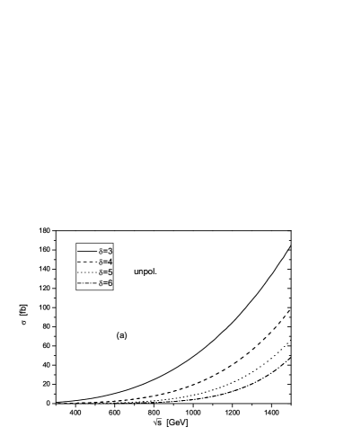
From Table 1 we can see that the cross section can reach several hundred $fb$ when the $\gamma-\gamma$ c.m.s. energy is 1 TeV. The larger the number of extra dimensions is, the smaller the cross section becomes. It is obvious that the cross sections in the case with + - polarized incoming photons are much larger than those in the case in + + polarized photon-photon collision. This is because the spin of the emitted graviton is 2, so it is much easier for J=2 initial states to generate a spin-2 graviton. This feature becomes more evident when the number of extra dimensions becomes larger. When $\delta=6$, the cross section with the + - polarized photons can reach three times of that with the + + polarized photons. We also find that the cross sections at $\sqrt{s}=1~{}{\rm TeV}$ are much larger than those at $\sqrt{s}=500~{}GeV$. To show the relationship between the cross section and the $\gamma-\gamma$ c.m.s energy more clearly, we depict two curves for the production rate of the process $\gamma\gamma\to e^{+}e^{-}G_{n}~{}$as the function of $\sqrt{s}$ in Fig.2, with ${\rm M_{S}=1.5~{}TeV}$ and the incoming photons being unpolarized and + - polarized($P_{\gamma}$=0.9), respectively. Since the perturbative theory is only applicable when $\sqrt{s}\leq{\rm M_{S}}$, we take the $\sqrt{s}<1.5~{}{\rm TeV}$ in Fig.2. The figure shows that the cross sections go up quickly with the increment of $\sqrt{s}$, because there are more KK-states contribute to the cross section. And the cross section is rather small at low $\sqrt{s}$ because of phase space suppression. At the same time we can see that the $+~{}-$ polarization photon beams can strongly enhance the cross section.

Figure 2: The cross section for process $\gamma\gamma\to e^{+}e^{-}G_{n}~{}$as the functions of $\gamma\gamma$ colliding energy $\sqrt{s}$, with ${\rm M_{S}=1.5~{}TeV}$. (a) for the unpolarized photon-photon collision, (b) for + - polarized photon-photon collision with $P_{\gamma}=0.9$.

III Signal analysis

Since graviton interacts with materials weakly, an emitted graviton cannot be detected in experiment. Therefore, in the measurement of the process $\gamma\gamma\to e^{+}e^{-}G_{n}~{}$the existence of a graviton manifests as the phenomenon of missing energy. The signature for this process is:

$$\gamma\gamma\to e^{+}e^{-}+missing~{}energy.$$ (3.1)

So the processes of the form $\gamma\gamma\to e^{+}e^{-}(neutrinos)$, where the neutrinos can be of any generation, are $SM$ background which can effect the discrimination of the graviton. The main $SM$ background processes at the lowest order for the signal of $\gamma\gamma\to e^{+}e^{-}G_{n}~{}$are:

$$\gamma\gamma\to e^{+}e^{-}$$ (3.2)

$$\gamma\gamma\to e^{+}e^{-}Z\to e^{+}e^{-}(\nu\bar{\nu})$$ (3.3)

$$\gamma\gamma\to W^{+}W^{-}\to(e^{+}\nu_{e})(e^{-}\bar{\nu_{e}})$$ (3.4)

$$\gamma\gamma\to\tau^{+}\tau^{-}\to(e^{+}\nu_{e}\bar{\nu_{\tau}})(e^{-}\bar{\nu_{e}}\nu_{\tau})$$ (3.5)

All these processes contribute a formidable background to the graviton signal of $\gamma\gamma\to e^{+}e^{-}G_{n}~{}$. However, a reasonable set of kinematic cuts enable us to distinguish the suggested signal from the backgrounds. Firstly, the electron-positron pair in the process (3.2) are collinear, so we can remove the $\gamma\gamma\to e^{-}e^{+}$ background totally by putting a cut on the angle between the final electron and positron. The contributions from $\gamma\gamma\to e^{+}e^{-}Z$ can be expressed as:

$$\sigma_{e^{+}e^{-}Z} = \sigma(\gamma\gamma\to e^{+}e^{-}Z)\times Br(Z\to\nu\bar{\nu})$$ (3.6)

$$= \sigma(\gamma\gamma\to e^{+}e^{-}Z)\times 20.0\%$$

$$= \cases{10.65~{}fb~{}~{}~{}~{}~{}(for~{}\sqrt{s}=500~{}GeV);\cr 4.17~{}fb~{}~{}~{}~{}~{}(for~{}\sqrt{s}=1000~{}GeV).}$$ (3.7)

The primary dominant backgrounds should be the $\gamma\gamma\to W^{+}W^{-}$ and $\gamma\gamma\to\tau^{+}\tau^{-}$ processes, which are called as WW- and $\tau\tau$-background respectively in the following discussion. Their contributions are given by

$$\sigma_{WW} = \sigma(\gamma\gamma\to W^{+}W^{-})\times\left(Br(W\to e\nu_{e})\right)^{2}$$ (3.8)

$$= \sigma(\gamma\gamma\to W^{+}W^{-})\times(10.75\%)^{2}$$

$$= \cases{1011~{}fb~{}~{}~{}~{}~{}(for~{}\sqrt{s}=500~{}GeV)\cr 1019~{}fb~{}~{}~{}~{}~{}(for~{}\sqrt{s}=1000~{}GeV).}$$ (3.9)

$$\sigma_{\tau\tau} = \sigma(\gamma\gamma\to\tau^{+}\tau^{-})\times\left(Br(\tau\to e\nu_{e}\nu_{\tau})\right)^{2}$$ (3.10)

$$= \sigma(\gamma\gamma\to\tau^{+}\tau^{-})\times(17.84\%)^{2}$$

$$= \cases{243.1~{}fb~{}~{}~{}~{}~{}(for~{}\sqrt{s}=500~{}GeV)\cr 62.36~{}fb~{}~{}~{}~{}~{}(for~{}\sqrt{s}=1000~{}GeV).}$$ (3.11)

We developed an event generator program for the process $\gamma\gamma\to e^{+}e^{-}G_{n}~{}$and $\gamma\gamma\to e^{+}e^{-}Z$, and the WW- and $\tau\tau$-background events are generated by adopting Pythia package[18]. In Fig.3 we depict the Monte Carlo distributions of the open angle between electron and positron $\theta_{ee}$ for the signal process $\gamma\gamma\to e^{+}e^{-}G_{n}~{}$and background processes($\gamma\gamma\to e^{+}e^{-}Z$, $\gamma\gamma\to W^{+}W^{-}$ and $\gamma\gamma\to\tau\tau$) separately, with the $\gamma\gamma$ colliding energy $\sqrt{s}=1~{}{\rm TeV}$. The $\theta_{ee}$ distributions for the signal process $\gamma\gamma\to e^{+}e^{-}G_{n}~{}$, $\gamma\gamma\to e^{+}e^{-}Z$, WW- and $\tau\tau$-background processes at $\sqrt{s}=500~{}{\rm GeV}$ have the similar line-shapes with the corresponding ones at $\sqrt{s}=1000~{}{\rm GeV}$ as shown in Fig.3. The back-to-back feature of the final $e^{+}e^{-}$ pair for the main background processes is shown evidently in Fig.3, especially for the process $\gamma\gamma\to\tau\tau$. If we put a suitable cut on the open angle between the electron and positron $\theta_{ee}^{cut}$, it is possible to remove the background events including also the $\gamma\gamma\to e^{+}e^{-}$ process from the signals of $\gamma\gamma\to e^{+}e^{-}G_{n}~{}$at $\sqrt{s}=1000~{}{\rm GeV}$. But in the case of $\sqrt{s}=500~{}{\rm GeV}$, the $\theta_{ee}^{cut}$ is not enough to eliminate WW-background process. In Fig.4 we show the simulating distributions of the missing invariant mass of the signal process $\gamma\gamma\to e^{+}e^{-}G_{n}~{}$and the WW-background process with extra dimensions $\delta=3$, $\sqrt{s}=500~{}GeV$ and ${\rm M_{S}=1~{}TeV}$ after applying $CUT1$ which is introduced below, and find that an extra missing invariant mass cut can reduce more WW-background events.

Figure 3: Distributions of the open angel between the electron and positron for the signal process when extra dimensions $\delta=3$ and the background processes. The $\gamma\gamma$ c.m.s. energy is 1 TeV and ${\rm M_{S}}$ is set to be 1 TeV.

Figure 4: Distributions of the missing invariant mass of the signal process and the WW-background process after applying $CUT1$ when extra dimensions $\delta=3$. The $\gamma\gamma$ c.m.s. energy is $500~{}GeV$ and ${\rm M_{S}}$ is set to be 1 TeV.

From the above discussion we choose the off-line event selection criterions as follows:

1. To take into account the detector acceptance, firstly, we demand that the angle between electron(positron) and the photon beam should be in the range $5^{\circ}<\theta_{e\gamma}<175^{\circ}$. Secondly, the transverse momentum of the electron(positron) should satisfy $p_{T}^{e}>5~{}{\rm GeV}$. We also demand that the electron(positron) energy $E_{e}>1GeV$. To separate the electron and positron tracks, we demand that the open angle between electron and positron $\theta_{ee}$ should be large than $5^{\circ}$. On the other hand, to eliminate the WW, $\tau\tau$, $\gamma\gamma\to e^{+}e^{-}$ and $e^{+}e^{-}Z$ background, we set a more strict cut on $\theta_{ee}$, i.e., $5^{\circ}<\theta_{ee}<\theta_{ee}^{cut}=90^{\circ}$. We denote these cuts as $CUT1$ set, which are expressed as

   $$5^{\circ}<\theta_{e\gamma}<175^{\circ},~{}p_{T}^{e}>5~{}GeV,~{}E_{e}>1~{}GeV,~{}{\rm and}~{}5^{\circ}<\theta_{ee}<\theta_{ee}^{cut}=90^{\circ}$$

2. For $\sqrt{s}=500~{}{\rm GeV}$, a cut on the missing invariant mass is needed, which is denoted as $CUT2$:

   $$M_{miss}<400~{}GeV$$

Taking the photon integrated luminosity to be ${\cal L}=100^{-1}fb$, we present in Table 2 the event numbers of the signal process with $\delta=3$ and ${\rm M_{S}=1~{}TeV}$ and the background processes after each step of cut, the event selection efficiency after cuts, and the significance of signal over background. Here the event selection efficiency is defined as the event numbers after cuts divided by the event numbers before any cut. The significance of signal over background is defined as

$$SB = \frac{N_{signal}}{\sqrt{N_{background}}}=\frac{\sigma_{S}^{CUT}\cdot{\cal L}_{\gamma\gamma}}{\sqrt{\sigma_{B}^{CUT}\cdot{\cal L}_{\gamma\gamma}}}$$

$$= \frac{\sigma_{S}^{CUT}}{\sqrt{\sigma_{B}^{CUT}}}\cdot\sqrt{{\cal L}_{\gamma\gamma}}$$

Table 2: Event selection on background and signal($\delta=3$) with unpolarization case.

	$\sqrt{s}=500GeV$				$\sqrt{s}=1000GeV$
	$e^{+}e^{-}G_{n}$	WW	$\tau\tau$	$e^{+}e^{-}Z$	$e^{+}e^{-}G_{n}$	WW	$\tau\tau$	$e^{+}e^{-}Z$
N before cut	4646	101100	24310	1065	37170	101900	6236	417
N after $CUT1$	1805	5402	0	86	17790	649	0	31
N after $CUT2$	1616	3427	0	86	/	/	/	/
efficiency $\epsilon$	34.8%	3.39%	0%	8.08%	47.9%	0.64%	0%	7.43%
SB	27.26				682.2

Here we have discussed the case of unpolarized photons. In Section II we show that the cross section for the signal process with $J=2$ polarized photons is much larger than that with $J=0$ photons. On the contrary, we find that with the incoming photon polarizations, the cross section for the primary $SM$ background process $\gamma\gamma\to W^{+}W^{-}$ is suppressed in the colliding case with $J=2$. So it will be much easier to eliminate $SM$ backgrounds in case of $J=2$ collision mode. Using the similar signal analysis procedure with above, we obtain the data with $+-$ polarized case(with $P_{\gamma}=0.9$), and list them in Table 3.

Table 3: Event selection on background and signal($\delta=3$),with $+-$ polarized photon beams($P_{\gamma}=0.9$).

	$\sqrt{s}=500GeV$				$\sqrt{s}=1000GeV$
	$e^{+}e^{-}G_{n}$	WW	$\tau\tau$	$e^{+}e^{-}Z$	$e^{+}e^{-}G_{n}$	WW	$\tau\tau$	$e^{+}e^{-}Z$
N before cut	5926	96159	38271	1340	47400	99065	10299	480
N after $CUT1$	2104	5152	0	59	21524	631	0	19
N after $CUT2$	1782	3268	0	59	/	/	/	/
efficiency $\epsilon$	30.1%	3.40%	0%	4.40%	45.4%	0.64%	0%	3.96%
SB	30.89				844.2

Notice that the data in Table 2 and Table 3 are obtained by taking ${\rm M_{S}=1~{}TeV}$. The cross section of the signal process is proportional to $1/M_{S}^{\delta+2}$(see Eq.(2.10-2.11)), so the SB value is proportional to $1/M_{S}^{\delta+2}$, too. If we suppose that the signature can be detected only when $SB\geq 5$ in experiment, then we can reach the conclusion that in the case of $\sqrt{s}=1~{}{\rm TeV}$, $\delta=3$ and unpolarized photon beams, graviton signal can be detected when ${\rm M_{S}}\leq 2.67~{}{\rm TeV}$, while in the case of $\sqrt{s}=500~{}{\rm GeV}$, the graviton signal can be detected only when ${\rm M_{S}}\leq 1.40~{}{\rm TeV}$. These limits are increased to 2.79 ${\rm TeV}$(when $\sqrt{s}=1~{}{\rm TeV}$) and 1.44 ${\rm TeV}$(when $\sqrt{s}=500~{}{\rm GeV}$) in $+-$ polarized photon collision mode with $P_{\gamma}=0.9$, respectively.

IV Summary

In this paper we calculate the cross sections for the process $\gamma\gamma\to e^{+}e^{-}G_{n}~{}$in different polarized photon collision modes, and present some strategies to discriminate the graviton signal from numerous $SM$ backgrounds.

At the stage of ILC with $\sqrt{s}=1~{}{\rm TeV}$, the cross section for the process $\gamma\gamma\to e^{+}e^{-}G_{n}~{}$can reach several hundred $fb$. Because the spin of the emitted graviton is 2, the $\gamma\gamma$ collision with $J=2$ strongly enhances the production rate of process $\gamma\gamma\to e^{+}e^{-}G_{n}~{}$, especially when the number of extra dimensions is large. Of course, the cross section increases with the increment of c.m.s. energy $\sqrt{s}$, due to more KK-states exist which contribute to the cross section. Another effect of the $LED$ shown in this paper is that the cross section decreases when the number of extra dimensions $\delta$ goes up.

For the case of $\delta=3$, we present some strategies to select graviton signals from the numerous $SM$ backgrounds. Because most of the $e^{+}e^{-}$ pair of the background processes are back-to-back, taking cut on the open angle between electron and positron can reduce the backgrounds efficiently. With our suggested event selection criterions, we can reach rather high $SB$ value. We conclude that by adopting an unpolarized $\gamma\gamma$ collision machine with $\sqrt{s}=1~{}{\rm TeV}$ in the case of $\delta=3$ and ${\cal L}=100fb^{-1}$, the graviton signal can be detected when ${\rm M_{S}}\leq 2.67~{}{\rm TeV}$, while in the case of $\sqrt{s}=500~{}{\rm GeV}$, the graviton signal can be detected only when ${\rm M_{S}}\leq 1.40~{}{\rm TeV}$. If we adopt a $\gamma\gamma$ collider machine in $+-$ polarized photon collision mode, the detecting upper limits on the fundamental scale can be improved up to 2.79 ${\rm TeV}$ when $\sqrt{s}=1~{}{\rm TeV}$, and 1.44 ${\rm TeV}$ when $\sqrt{s}=0.5~{}{\rm TeV}$.

Acknowledgments: This work was supported in part by the National Natural Science Foundation of China, the Education Ministry of China and a special fund sponsored by Chinese Academy of Sciences.

References

• [1] N. Arkani-Hamed, S. Dimopoulos and G. R. Dvali, Phys. Lett. B 429 (1998) 263 [arXiv:hep-ph/9803315]; I. Antoniadis, N. Arkani-Hamed, S. Dimopoulos and G. R. Dvali, Phys. Lett. B 436 (1998) 257 [arXiv:hep-ph/9804398]; N. Arkani-Hamed, S. Dimopoulos and G. R. Dvali, Phys. Rev.  D 59, 086004 (1999) [arXiv:hep-ph/9807344].
• [2] J. D. Lykken, Phys. Rev.  D 54, 3693 (1996) [arXiv:hep-th/9603133].
• [3] E. Witten, Nucl. Phys.  B 471, 135 (1996) [arXiv:hep-th/9602070].
• [4] P. Horava and E. Witten, Nucl. Phys.  B 460, 506 (1996) [arXiv:hep-th/9510209]; Nucl. Phys.  B 475, 94 (1996) [arXiv:hep-th/9603142].
• [5] I. Antoniadis, Phys. Lett.  B 246, 377 (1990).
• [6] L. Randall and R. Sundrum, Phys. Rev. Lett.  83, 3370 (1999) [arXiv:hep-ph/9905221]; Phys. Rev. Lett.  83, 4690 (1999) [arXiv:hep-th/9906064].
• [7] D. J. Kapner, T. S. Cook, E. G. Adelberger, J. H. Gundlach, B. R. Heckel, C. D. Hoyle and H. E. Swanson, Phys. Rev. Lett.  98, 021101 (2007) [arXiv:hep-ph/0611184].
• [8] G. F. Giudice, R. Rattazzi and J. D. Wells, Nucl. Phys.  B 544, 3 (1999) [arXiv:hep-ph/9811291].
• [9] T. Han, J. D. Lykken and R. J. Zhang, Phys. Rev.  D 59, 105006 (1999) [arXiv:hep-ph/9811350].
• [10] G. Weiglein et al. [LHC/LC Study Group], Phys. Rept.  426, 47 (2006) [arXiv:hep-ph/0410364].
• [11] E. A. Mirabelli, M. Perelstein and M. E. Peskin, Phys. Rev. Lett.  82, 2236 (1999) [arXiv:hep-ph/9811337].
• [12] M. Besancon, arXiv:hep-ph/9909364.
• [13] S. Dutta, P. Konar, B. Mukhopadhyaya and S. Raychaudhuri, Phys. Rev.  D 68, 095005 (2003) [arXiv:hep-ph/0307117].
• [14] D. Atwood, S. Bar-Shalom and A. Soni, Phys. Rev.  D 61, 116011 (2000) [arXiv:hep-ph/9909392].
• [15] K. m. Cheung and W. Y. Keung, Phys. Rev.  D 60, 112003 (1999) [arXiv:hep-ph/9903294].
• [16] V. I. Telnov, “Physics options at the ILC. GG6 summary at Snowmass2005,” arXiv:physics/0512048; V. I. Telnov, Acta Phys. Polon.  B 37, 633 (2006) [arXiv:physics/0602172].
• [17] A. V. Pak, D. V. Pavluchenko, S. S. Petrosyan, V. G. Serbo and V. I. Telnov, Nucl. Phys. Proc. Suppl.  126, 379 (2004) [arXiv:hep-ex/0301037].
• [18] T. Sjostrand et al., High-energy-physics event generation with pythia 6.1, Computer Phys. Commun. 135(2001)238 [hep-ph/0010017]
• [19] S. Eidelman, et al., Phys. Lett. B592(2004)1.
• [20] K.Hagiwara et al, Phys.ReV.D66(2002)1.