Constraining the geometry of the neutron star RX J1856.5$-$3754

Abstract

RX J1856.5$-$3754 is one of the brightest, nearby isolated neutron stars, and considerable observational resources have been devoted to its study. In previous work, we found that our latest models of a magnetic, hydrogen atmosphere matches well the entire spectrum, from X-rays to optical (with best-fitting neutron star radius $R\approx 14$ km, gravitational redshift $z_{g}\sim 0.2$, and magnetic field $B\approx 4\times 10^{12}$ G). A remaining puzzle is the non-detection of rotational modulation of the X-ray emission, despite extensive searches. The situation changed recently with XMM-Newton observations that uncovered 7 s pulsations at the $\approx 1\%$ level. By comparing the predictions of our model (which includes simple dipolar-like surface distributions of magnetic field and temperature) with the observed brightness variations, we are able to constrain the geometry of RX J1856.5$-$3754, with one angle $<6^{\circ}$ and the other angle $\approx 20-45^{\circ}$, though the solutions are not definitive given the observational and model uncertainties. These angles indicate a close alignment between the rotation and magnetic axes or between the rotation axis and the observer. We discuss our results in the context of RX J1856.5$-$3754 being a normal radio pulsar and a candidate for observation by future X-ray polarization missions such as Constellation-X or XEUS.

1 Introduction

Seven candidate isolated, cooling neutron stars (INSs) have been identified by the ROSAT All-Sky Survey (see Kaspi, Roberts, & Harding 2006; Haberl 2007; van Kerkwijk & Kaplan 2007, for recent reviews). These objects share the following properties: (1) high X-ray to optical flux ratios of $\log(f_{\rm X}/f_{\rm optical})\sim 4-5.5$, (2) soft X-ray spectra that are well described by blackbodies with $kT\sim 50-100$ eV, (3) relatively steady X-ray flux over long timescales, and (4) lack of radio pulsations.

For the particular INS RX J1856.5$-$3754, X-ray and optical/UV data can be well-fit by two corresponding blackbody spectra: the X-ray spectrum by a blackbody with $kT^{\infty}_{\rm X}=63$ eV and emission size $R^{\infty}_{\rm X}=5.1\,(d/\mbox{140 pc})$ km, and the optical/UV spectrum by a blackbody with $kT^{\infty}_{\rm opt}=26$ eV, and $R^{\infty}_{\rm opt}=21.2\,(d/\mbox{140 pc})$ km (Burwitz et al. 2001; van Kerkwijk & Kulkarni 2001a; Drake et al. 2002; see also Pavlov, Zavlin, & Sanwal 2002; Trümper et al. 2004; Walter 2004), where $T^{\infty}=T_{\rm eff}/(1+z_{g})$, $R^{\infty}=R^{\rm em}(1+z_{g})$, $R^{\rm em}$ is the physical size of the emission region, and $d$ is the distance. The gravitational redshift $z_{g}$ is given by $(1+z_{g})=(1-2GM/Rc^{2})^{-1/2}$, where $M$ and $R$ are the mass and radius of the NS, respectively. The high temperature, small area X-ray blackbody suggests a small hot spot on the NS surface, while the optical blackbody with $R^{\infty}_{\rm opt}$ is the remaining large, cool surface.

Even though blackbody spectra fit the data, one expects NSs to possess atmospheres of either heavy elements (due to debris from the progenitor) or light elements (due to gravitational settling or accretion). The lack of any significant spectral features in the X-ray spectrum argues against a heavy element atmosphere (Burwitz et al. 2001, 2003), whereas non-magnetic or fully-ionized magnetic hydrogen atmosphere spectra do not provide a good fit (Pavlov et al. 1996; Pons et al. 2002; Burwitz et al. 2001, 2003). For the last case, it is important to note that, since $kT\sim\mbox{tens of}$ eV for RX J1856.5$-$3754 and the ionization energy of hydrogen at $B=10^{12}$ G is 160 eV, the presence of neutral atoms must be accounted for in the magnetic hydrogen atmosphere models; the opacities are sufficiently different from the fully ionized opacities that they can change the atmosphere structure and continuum flux (Ho et al. 2003; Potekhin et al. 2004), which can affect fitting of the observed spectra (see, e.g., Ho et al. 2007).

Another issue that may argue against the two-temperature blackbody model is the the non-detection, until recently, of X-ray pulsations due to the rotation of the NS (down to the 1.3% level; Drake et al. 2002; Ransom, Gaensler, & Slane 2002; Burwitz et al. 2003; Zavlin 2007). As discussed in the important work by Braje & Romani (2002), very low rotational pulsations could be due to a very close alignment between the rotation and magnetic axes and/or an unfavorable viewing geometry. Assuming blackbody emission, they find this is possible in $\sim 5\%$ of viewing geometries (with $R=14$ km). However, more realistic atmosphere emission can lead to enhancement of pulsations, as well as an energy-dependence of the pulsations (see below).

Thus there existed three major observational and theoretical inconsistencies: (1) the inferred emission size from blackbody fits are either much smaller ($R^{\infty}\sim 5$ km from the X-ray data) or much larger ($R^{\infty}\sim 20$ km from the optical/UV data) than the canonical NS radius of $10-12$ km, even after correcting for the redshift, (2) blackbodies fit the spectrum much better than realistic atmosphere models, and (3) strong upper limits on X-ray pulsations suggest RX J1856.5$-$3754 may have a largely uniform temperature over the entire NS surface. In response to these problems, we applied our latest magnetic, partially-ionized hydrogen atmosphere models and obtained a good fit to the entire multi-wavelength spectrum of RX J1856.5$-$3754 (Ho et al. 2007; hereafter H07). Besides using the more realistic atmosphere, the fit requires a smaller emission size $R^{\rm em}\approx 14$ km (as compared to the blackbody models); if interpreted as emission from the entire NS, the size can be satisfied by a stiff but standard equation of state (see, e.g., Lattimer & Prakash 2007). Furthermore, we found geometries that produce pulsations near the observed limits. Because of observational uncertainties and the computationally tedious task of constructing a complete grid of models, the results may not be unique. Nevertheless, our model represents the most self-consistent picture for explaining all the observations of RX J1856.5$-$3754.

Very recently, XMM-Newton observations uncovered pulsations from RX J1856.5$-$3754 with a period of 7 s (pulse amplitude $\approx 1\%$) and an upper limit on the period derivative; by assuming vacuum magnetic dipole braking, this implies $B<10^{14}$ G (Tiengo & Mereghetti 2007; hereafter TM07). The detection of pulsations allows us to constrain the geometry (i.e., two angles $\alpha$ and $\zeta$, where $\alpha$ is the angle between the rotation and magnetic axes and $\zeta$ is the angle between the rotation axis and the direction to the observer) through a comparison of the observed brightness variations ($\equiv$ light curves) with those implied by the model of H07; the latter are obtained by computing the (rotation) phase-dependent spectra from the entire NS surface.

Spectra from the whole NS surface are necessarily model-dependent (see, e.g., Zavlin et al. 1995; Zane et al. 2001; Ho & Lai 2004; Zane & Turolla 2006), as the magnetic field and temperature distributions over the NS surface are unknown. Magnetic field variations over the surface will induce surface temperature variations (Greenstein & Hartke 1983). Furthermore, radiation from the surface of a magnetic NS with an atmosphere differs significantly from that implied by isotropic blackbody emission: the emission depends on the direction of the local surface magnetic field (Shibanov et al. 1992; Pavlov et al. 1994). Indeed, there have been recent works attempting to fit magnetic atmosphere spectra to observations of NSs other than RX J1856.5$-$3754. Lloyd et al. (2003) fit the spectrum and light curve of PSR 0656+14, while Zavlin & Pavlov (2004), using a different model, do the same for PSR B0950+08. Zane & Turolla (2006), using the method of Lloyd et al. (2003) to produce an extensive library of light curves for fully ionized hydrogen atmospheres, fit the light curves of several INSs.

An outline of the paper is as follows. In Section 2, we describe the model used to produce light curves of RX J1856.5$-$3754. Light curves for arbitrary angles ($\alpha,\zeta$) are discussed in Section 3. The observations and fits to the observations are shown in Section 4. We summarize and discuss our results in Section 5.

2 Model for Neutron Star Emission

We adopt a relatively simple model (see also Zavlin et al. 1995; Lloyd et al. 2003) for the surface magnetic field $B$ and effective temperature $T_{\rm eff}$ distributions: we assume the surface is symmetric (in $B$ and $T_{\rm eff}$) about the magnetic equator and divide the hemisphere into four magnetic colatitudinal regions. We generate (local) atmosphere models (see H07, and references therein, for details; see Zavlin & Pavlov 2002, for a review of atmosphere modeling) for each region with the parameters given in Table 1, where $\Theta_{B}$ is the angle between the local magnetic field and the surface normal. Emission from any point within a colatitudinal region is given by the atmosphere model for that region. Note that the magnetic field distribution is roughly dipolar. The phase-resolved spectra and light curves from the entire NS surface is then calculated by the method described below (see the analogous formalism in Pavlov & Zavlin 2000). We assume $M=1.4M_{\odot}$ and $R=14$ km (see H07). This implies $z_{g}=0.2$, and all energies quoted in this work have been redshifted from the local NS frame by this factor.

Table 1: Parameters for Neutron Star Surface

magnetic colatitude	$B$	$\Theta_{B}$	$T_{\rm eff}$
(deg)	($10^{12}$ G)	(deg)	($10^{5}$ K)
0$-$10	6	0	7
10$-$40	5	30	6
40$-$70	4	60	5
70$-$90	3	90	4

The observed emission from a local region (e.g., the hot magnetic polar cap) of a rotating NS depends on two angles: the angle $\alpha$ between the rotation and magnetic pole axes and the angle $\zeta$ between the rotation axis and the line-of-sight to the observer. In the coordinate frame $\mathbf{x}$, where $\hat{\mathbf{z}}$ is the direction to the observer and the spin axis $\mathbf{\Omega}_{\rm s}$ is in the $\hat{\mathbf{x}}\hat{\mathbf{z}}$-plane, the polar angle $\theta_{m}$ and azimuthal angle $\phi_{m}$ of the magnetic pole $\mathbf{m}$ are given by

$$\cos\theta_{m} = \cos\phi_{\rm p}\sin\alpha\sin\zeta+\cos\alpha\cos\zeta$$ (1)

$$\tan\phi_{m} = \frac{\sin\phi_{\rm p}\sin\alpha}{\cos\phi_{\rm p}\sin\alpha\cos\zeta-\cos\alpha\sin\zeta},$$ (2)

respectively (see Figure 1). $\phi_{\rm p}$ ($=\Omega_{\rm s}t$) is the rotation phase. Note that the light curves are symmetric under the interchange of $\alpha$ and $\zeta$, since the brightness depends only on the angle $\theta_{m}$ between the magnetic and line-of-sight axes. At the emission-point P [=P($\theta,\phi$)] on the NS surface (see Figure 1), the direction of the local magnetic field $\mathbf{B}$ (assuming a magnetic dipole geometry) is given by

$$\cos\Theta_{B}=\cos(\phi_{m}-\phi)\sin\theta\sin\theta_{m}+\cos\theta\cos\theta_{m}$$ (3)

$$\tan\phi_{k}=\frac{\sin(\phi_{m}-\phi)\sin\theta_{m}}{\cos(\phi_{m}-\phi)\cos\theta\sin\theta_{m}-\sin\theta\cos\theta_{m}}.$$ (4)

$\phi_{k}$ is the azimuthal angle between $\mathbf{B}$ and the photon wavevector $\mathbf{k}$ and is defined in the coordinate frame $\mathbf{x}_{\rm n}$, where $\hat{\mathbf{z}}_{\rm n}$ is the direction of the surface normal and $\mathbf{k}$ is in the $\hat{\mathbf{x}}_{\rm n}\hat{\mathbf{z}}_{\rm n}$-plane.

Figure 1: Coordinate axes and angles used to describe the pulsed emission. The observer is in the $\hat{\mathbf{z}}$-direction. The dashed line indicates the position of the magnetic pole $\mathbf{m}$ as the neutron star rotates about $\mathbf{\Omega}_{\rm s}$.

To determine the flux spectrum $F_{E}$ for a given rotation phase, we first compile a table of specific intensities $I_{E}(\theta_{k},\phi_{k})$, where $\theta_{k}$ is the angle between $\mathbf{k}$ and $\hat{\mathbf{z}}_{\rm n}$. $I_{E}$ are computed from atmosphere models described in H07; these models depend on the local effective temperature and magnetic field direction $\Theta_{B}$ and strength (see Table 1). The flux spectrum can then be calculated from

$$F_{E}=\left(\frac{R^{\infty}}{d}\right)^{2}\frac{1}{(1+z_{g})^{3}}\int_{0}^{2\pi}d\phi_{k}\int_{0}^{1}d\mu_{k}\,\mu_{k}I_{E}(\theta_{k},\phi_{k}),$$ (5)

where $\mu_{k}=\cos\theta_{k}$. In the absence of the bending of the path of light due to gravity, the polar angles of the emission-point and the photon wavevector are the same, i.e., $\theta=\theta_{k}$. Gravitational light-bending causes more of the NS surface to be visible (for $M=1.4M_{\odot}$ and $R=14$ km, $\theta\leq 115^{\circ}$ as compared to $\leq 90^{\circ}$ without light-bending). We use the approximate relation between $\theta$ and $\theta_{k}$ given in Beloborodov (2002)

$$\cos\theta=\frac{\cos\theta_{k}-2GM/c^{2}R}{1-2GM/c^{2}R},$$ (6)

which deviates from the exact relation given in Pechenick, Ftaclas, & Cohen (1983) by $\lesssim 1\%$ for our chosen $M$ and $R$. The light curves are then computed by integrating the photon count spectra over the energy range of the XMM-Newton observations (see TM07): 0.15$-$1.2 keV for the total X-ray spectrum, 0.15$-$0.26 keV for the soft band, and 0.26$-$1.2 keV for the hard band.

3 Results

Figure 2 shows the light curves of our NS model for various geometries ($\alpha,\zeta$). We also plot the analytic light curves from Beloborodov (2002) for isotropic emission from two antipodal hot spots (see Zavlin & Pavlov 1998; Bogdanov, Rybicki, & Grindlay 2006, for examples of pulse profiles from non-magnetic hydrogen atmosphere hot spots). We refer to the region at magnetic colatitude 0$-$10^∘ as the primary magnetic polar cap and the opposite pole as the secondary cap. The classification scheme (for isotropically-emitting hot caps) is defined in Beloborodov (2002): (I) only the primary cap is visible, and the pulse profile is purely sinusoidal with a single peak, (II) the secondary cap is seen around pulse minimum due to relativistic light-bending, which reduces the strength of the modulation, (III) the primary cap is not seen during a segment of the rotation, and (IV) both spots are seen at all phases and thus there is no modulation. Relativistic light-bending allows $\theta\leq 115^{\circ}$ to be visible; thus, e.g., for (20^∘,80^∘), one pole will not be seen during a portion of the rotation.

Figure 2: Light curves for different geometries ($\alpha,\zeta$): class I with (20^∘,30^∘), class II with (30^∘,60^∘), class III with (60^∘,80^∘), and class IV with (10^∘,80^∘). $\alpha$ is the angle between the spin and magnetic axes, and $\zeta$ is the angle between the spin axis and the line-of-sight. The four classes are defined in Beloborodov (2002). The solid lines are for the magnetic model described in the text [dashed line is for (50^∘,50^∘)], while the dotted lines are analytic light curves (scaled arbitrarily in amplitude) for isotropic emission from two antipodal hot spots (see Beloborodov 2002).

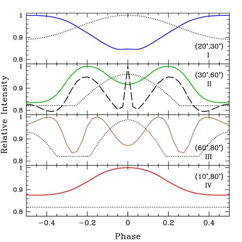
Several important features are evident from a comparison of magnetic atmosphere emission to that of isotropic emission. The ($\theta_{k},\phi_{k}$)-angular-dependence of the radiation (or beam pattern) manifests as a narrow “pencil-beam” along the direction of the magnetic field and a broad “fan-beam” at intermediate angles (see Pavlov et al. 1994; Lloyd 2003, for beam patterns and spectra at various $\Theta_{B}$ and $\phi_{k}$). As discussed in Pavlov et al. (1994), the pencil-beam is the result of the lower opacity at $\theta_{k}\lesssim(E/E_{B})^{1/2}$, where $E_{B}=\hbar eB/m_{\rm e}c=11.6\,(B/10^{12}\mbox{ G})$ keV is the electron cyclotron energy; the width of the pencil-beam is thus $\sim(E/E_{B})^{1/2}$, and the radiation is more strongly beamed at higher magnetic fields. For our case with $B\sim 4\times 10^{12}$ G, the width is $\sim 6^{\circ}$. This narrow beam is seen in the (50^∘,50^∘)-light curve plotted in Figure 2, which is the only instance shown that has the observer’s line-of-sight exactly crossing the magnetic cap and coinciding with the peak of the isotropic emission. Also evident is the fan-beam (most obvious in the light curves of classes II and III), which occur on either side of the magnetic cap and can increase the number of light-curve peaks. In addition, the anisotropic beam pattern (combined with the surface temperature variation) can produce an apparent phase shift compared to isotropic emission and modulation when an isotropic beam pattern suggests none (c.f. class IV).

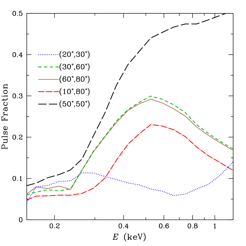
Figure 3 shows the pulse fractions, $PF=(C_{\rm max}-C_{\rm min})/(C_{\rm max}+C_{\rm min})$, where $C$ is the count spectrum, as a function of energy for various geometries. The energy-dependence of the light curves and pulse fractions is due to the energy-dependent beam patterns and the surface temperature and magnetic field variations. As noted in Zavlin et al. (1995), the pulse fraction is lower at low energies since the beam pattern is more isotropic. Phase shifts between the peak of the low and high-energy light curves can also occur.

Figure 3: Pulse fractions as a function of energy for different geometries ($\alpha,\zeta$) = (20^∘,30^∘), (30^∘,60^∘), (60^∘,80^∘), (10^∘,80^∘), (50^∘,50^∘). $\alpha$ is the angle between the spin and magnetic axes, and $\zeta$ is the angle between the spin axis and the line-of-sight.

4 Comparison to RX J1856.5$-$3754

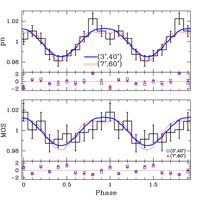
TM07 discovered 7 s pulsations in the 2006 October 24 observations of RX J1856.5$-$3754 made by the EPIC-pn and MOS cameras on XMM-Newton. These observations cover the energy range 0.15$-$1.2 keV. The pn light curve, with a pulse fraction of 1.6%$\pm$0.2%, is shown in Figure 4 and found to have no significant difference when divided into soft and hard energies; the MOS light curve is also shown in Figure 4 and found to be statistically consistent with no pulsations (TM07).

Figure 4: Energy-integrated (0.15$-$1.2 keV) light curves of RX J1856.5$-$3754. Histograms are the pn (top) and MOS (bottom) observations (see Fig. 1 of TM07). Solid and dotted lines are the models with ($3^{\circ}$,$40^{\circ}$) and ($7^{\circ}$,$60^{\circ}$), respectively, along with the fit deviations [i.e., (data-model)/$\sigma$] in the corresponding lower panels. Two rotation periods are shown for clarity.

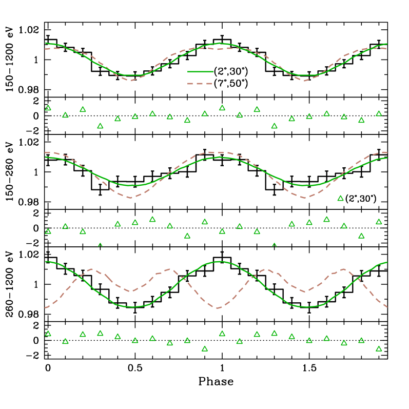
As a result of this discovery, TM07 analyzed previous XMM-Newton observations and found light curves that are consistent between the different observations; therefore these data were added together to obtain better statistics. Furthermore, when divided into soft (0.15$-$0.26 keV) and hard (0.26$-$1.2 keV) energy bands, the summed light curves demonstrate some energy-dependence, i.e., pulse fractions of $1.17\%\pm 0.08\%$ (0.15$-$1.2 keV), $0.88\%\pm 0.11\%$ (0.15$-$0.26 keV), and $1.5\%\pm 0.11\%$ (0.26$-$1.2 keV; see TM07). The light curves are shown in Figure 5.

Figure 5: Light curves of RX J1856.5$-$3754 for different energy ranges: 0.15$-$1.2 keV (top), 0.15$-$0.26 keV (middle), and 0.26$-$1.2 keV (bottom). Histograms are the light curves obtained by summing together all the XMM-Newton observations (see Fig. 4 of TM07). The solid lines are the model with ($2^{\circ}$,$30^{\circ}$), along with the fit deviations [i.e., (data-model)/$\sigma$] in the corresponding lower panels, while the dashed lines are the model with ($7^{\circ}$,$50^{\circ}$). Two rotation periods are shown for clarity.

Several characteristics of the observed light curves suggest possible values of $\alpha$ and $\zeta$: (1) the $\approx 1$% amplitude of the pulsations, (2) a single peak (or two peaks close in phase, as may be the case for the pn light curve in Figure 4) per rotation, and (3) no significant energy-dependence for the single observation (Figure 4) and small energy-dependence for the combined data (Figure 5). These characteristics imply the secondary cap is not a major contributor to the brightness variation (i.e., not class III) and small values of $\alpha$ or $\zeta$. Large $|\alpha-\zeta|$ are also implied since otherwise the pulsations would be strong with a narrow peak when the cap becomes aligned with the direction to the observer (a similar argument is made by Braje & Romani 2002 from the non-detection of RX J1856.5$-$3754 in the radio).

We compare the light curves generated from our model first to the single (2006 October 24) XMM-Newton observation and then to the summed data. To avoid the computational tedious task of computing light curves for a continuous distribution in the angles $\alpha$ and $\zeta$, we select specific values of ($\alpha,\zeta$), compute the light curve, and fit the model light curves to the observational data. The phase and normalization of the model light curves are arbitrary and are varied to minimize $\chi^{2}$. We restrict ourselves to integer values of ($\alpha,\zeta$) since the uncertainties in our model (see H07 and Section 5.1) and small variations between the data (c.f. Figures 4 and 5) do not warrant more detailed fits.

We obtain good fits to the 2006 October 24 observation with $\alpha$ and $\zeta$ of $\approx 2-9^{\circ}$ and $\sim 20-70^{\circ}$. Table 2 shows some of our fit results, where the pn data is fit with a model light curve and then the MOS data is fit using the same model light curve and phase alignment. Figure 4 illustrates two sample fits. These fits confine the allowed parameter space of ($\alpha,\zeta$). Furthermore, the light curves from this observation do not show significant differences when divided into soft and hard energies, whereas the model light curves with $\zeta\gtrsim 50^{\circ}$ show noticeably different hard-band pulsations. Therefore, the energy-(in)dependence of the data argues for $\zeta<50^{\circ}$.

Table 2: Fits to 2006 October 24 Light Curves

$\alpha^{({\rm a})}$	$\zeta^{({\rm a})}$	$\chi^{2}$/dof
(deg)	(deg)	pn(b)	MOS(c)
3	20	11.8/8	8.12/9
3	30	11.4/8	8.36/9
3	40	10.4/8	6.72/9
9	50	9.94/8	9.92/9
7	60	8.31/8	9.25/9
2	70	11.2/8	7.48/9

Notes:
(a) $\alpha$ and $\zeta$ are interchangeable.
(b) 10 phase bins $-$ 2 fit parameters (phase and normalization) = 8 dof
(c) The phase alignment from the pn fit is used.

Finally, we fit the (energy-dependent) light curves obtained by adding together the various XMM-Newton observations. Table 3 shows some of the results, where the total (0.15$-$1.2 keV) data is fit with a model light curve and then the soft (0.15$-$0.26 keV) and hard-band (0.26$-$1.2 keV) data is fit using the same phase alignment. The more stringent constraints on ($\alpha,\zeta$) are due to the better statistics and energy-dependence of the combined data. The model with ($\alpha,\zeta$)=($2^{\circ},30^{\circ}$) is shown in Figure 5.

Table 3: Fits to Combined Light Curves

$\alpha^{({\rm a})}$	$\zeta^{({\rm a})}$	$\chi^{2}$/dof
(deg)	(deg)	0.15$-$1.2 keV(b)	0.15$-$0.26 keV(c)	0.26$-$1.2 keV(c)
2	20	4.88/8	12.2/9	9.42/9
2	25	5.42/8	9.95/9	7.07/9
2	30	4.43/8	10.4/9	3.88/9
2	35	5.10/8	9.36/9	4.27/9
2	40	8.34/8	9.85/9	6.25/9
4	45	6.93/8	16.7/9	9.49/9

Notes:
(a) $\alpha$ and $\zeta$ are interchangeable.
(b) 10 phase bins $-$ 2 fit parameters (phase and normalization) = 8 dof
(c) The phase alignment from the 0.15$-$1.2 keV fit is used.

Figure 6: Pulse fractions as a function of $\zeta$ (or $\alpha$) for different $\alpha$ (or $\zeta$). The horizontal lines indicate the pulse fractions from TM07 using data from the 2006 October 24 observation and the combined observations; the shaded areas indicate the 1$\sigma$ uncertainty region.

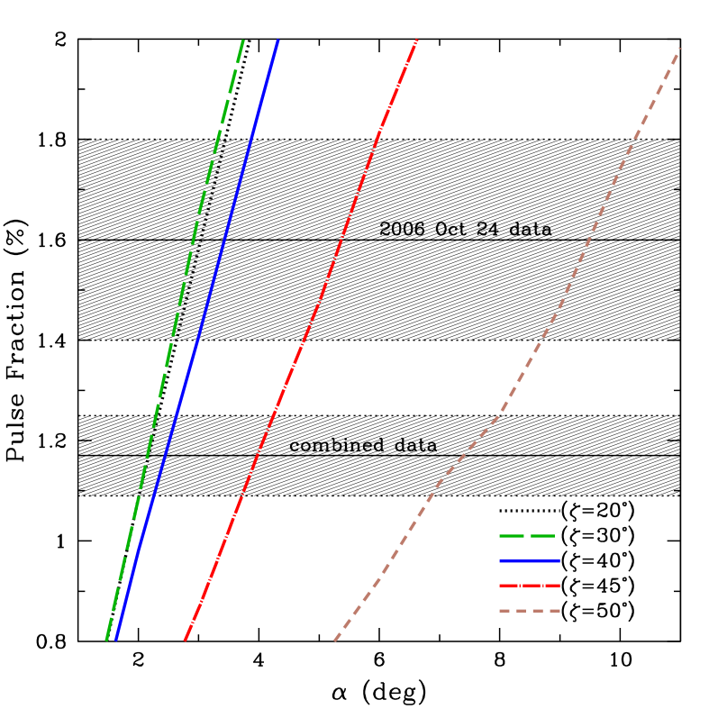
As an illustration of our fit results, we show in Figure 6 the ranges allowed by the 1$\sigma$ uncertainty in the measured pulse fractions and the pulse fractions of the model light curves as a function of $\alpha$ and $\zeta$. Only model light curves whose pulse fractions lie in the shaded regions can fit (within the uncertainties) the observed light curves. However, matching the pulse fraction is a necessary but not sufficient condition. As discussed above, the pulse shape and energy-dependence also serve as constraints. For example, it appears from Figure 6 that ($7^{\circ},50^{\circ}$) should fit the combined light curve. But the shape of the model light curve for this case is too broad and shows large differences when divided into soft and hard-energy bands (see Figure 5).

5 Discussion

In previous work (Ho et al. 2007), we successfully fit the multi-wavelength spectrum of RX J1856.5$-$3754 with our model of radiation from a magnetic neutron star containing a partially-ionized hydrogen atmosphere. With the recent discovery of rotational modulation of the X-ray emission (Tiengo & Mereghetti 2007), we use the light curves predicted by our model (which includes relatively simple surface distributions of the magnetic field and temperature) to constrain the geometry of RX J1856.5$-$3754. In particular, we find angles of $<6^{\circ}$ and $\approx 20-45^{\circ}$: one is the angle $\alpha$ between the rotation and magnetic axes and the other is the angle $\zeta$ between the rotation axis and the direction to the observer. Since the light curves with ($\alpha,\zeta$) are equivalent to those with ($\zeta,\alpha$), this implies that either the rotation and magnetic axes are closely aligned or we are essentially seeing down the spin axis of the neutron star (see also Braje & Romani 2002). We also note the following: (1) The model used here and described in Ho et al. (2007) assumes the high X-ray energy emission arises from a condensed iron surface below the hydrogen atmosphere. The emission properties of the condensed surface have been studied by Brinkmann (1980); Turolla, Zane, & Drake (2004); Pérez-Azorín, Miralles, & Pons (2005); van Adelsberg et al. (2005). (2) Though it would present an observational challenge, our model predicts optical pulsations with a singly-peaked sinusoid and pulse fractions of $\approx 0.1-0.5\%$. (3) Other members of the neutron star population RX J1856.5$-$3754 is thought to belong to show varying degrees of pulsations, some with a single peak (per rotation) and others with double peaks. Analyses of these sources will be presented in future work.

5.1 Changes in Surface Distributions of $B$ and $T_{\rm eff}$

We point out an uncertainty in our model that is difficult to quantify but will affect the light curves and thus the quality of the fits and the angles ($\alpha,\zeta$) inferred. We assume dipolar-like distributions of the magnetic field and temperature over the surface of the neutron star (see Table 1). If the size of each magnetic colatitudinal region is varied, the strength of the pulsations will change. For the geometries that best fit the observations, a $\pm 5^{\circ}$ change in the size of the the region described by $B=4\times 10^{12}$ G, $\Theta_{B}=60^{\circ}$, and $T_{\rm eff}=5\times 10^{5}$ K can result in a $\lesssim 0.002$ change in the pulse fraction, which is on the order of the observational errors. In addition, if the distributions are described by an offset dipole or if quadrupolar components are added on top of the dipole, then the shape and strength of the pulsations will, in general, be different.

5.2 RX J1856.5$-$3754 as a Normal Radio Pulsar?

One set of our solutions ($\alpha<6^{\circ}$) indicates a very close alignment between the rotation and magnetic axes. Observational evidence from studies of radio pulsars may also indicate the alignment of the rotation and magnetic axes on a timescale of $\sim 10^{7}$ y (Lyne & Manchester 1988; Tauris & Manchester 1998). For example, Tauris & Manchester (1998; see also Zhang, Jiang, & Mei 2003, and references therein) find the observed distribution of $\alpha$ peaks around $30-50^{\circ}$; after correcting for beaming, they find $\alpha$ decreases with time, with an average $\alpha\approx 40^{\circ}$ for pulsars younger than $10^{6.5}$ y. Thus both our solutions ($\alpha<6^{\circ}$ and $\alpha\approx 20-45^{\circ}$) fit within this scenario, given the $\sim 5\times 10^{5}$ y age of RX J1856.5$-$3754 (Kaplan, van Kerkwijk, & Anderson 2002; Walter & Lattimer 2002),

In spite of its non-detection at radio frequencies (Brazier & Johnston 1999), suppose RX J1856.5$-$3754 is a normal radio pulsar. The size of the radio beam $\rho$ is estimated to be $\rho\approx 5-6^{\circ}(P/\mbox{1 s})^{-1/2}=2^{\circ}$ (see, e.g., Rankin 1993; Gould 1994). Our results allow the radio beam to miss our line-of-sight, with the ($\alpha\approx 20-45^{\circ},\zeta<6^{\circ}$)-solution having a easier chance for this to occur. In addition, if RX J1856.5$-$3754 is losing rotational energy by magnetic dipole radiation, the spindown rate is $\dot{P}=10^{-15}\mbox{ s s${}^{-1}$}(B/\mbox{10${}^{12}$ G})^{2}(P/\mbox{1 s})^{-1}=5\times 10^{-15}\mbox{ s s${}^{-1}$}$, which is well below the $\dot{P}<1.9\times 10^{-12}\mbox{ s s${}^{-1}$}$ obtained by Tiengo & Mereghetti (2007). This spindown rate (and $\sim 5\times 10^{5}$ y age) implies that RX J1856.5$-$3754 must have been born at roughly its current spin period if no significant change in $\dot{P}$ (or $B$) occurred over its lifetime. Also, an H$\alpha$ nebula was found around RX J1856.5$-$3754 and has an estimated luminosity of $\dot{E}_{\rm bow}=8\times 10^{32}$ ergs s^-1 (van Kerkwijk & Kulkarni 2001b); the dipole spindown luminosity of RX J1856.5$-$3754 is insufficient in powering this relativistic wind. However, it is important to note in the above considerations that, given its spin period and magnetic field, RX J1856.5$-$3754 falls below the death line for radio pulsars; the death line being the region in $P-B$-space (or $P-\dot{P}$) where pulsars no longer emit in the radio (see, e.g., Sturrock 1971; Chen & Ruderman 1993; Harding, Muslimov, & Zhang 2002).

5.3 X-ray Polarization

In the presence of magnetic fields typical of isolated neutron stars such as RX J1856.5$-$3754 ($B\ga 10^{12}$ G), radiation propagates in two polarization modes: the ordinary mode is polarized parallel to the $\mathbf{k}$-$\mathbf{B}$ plane, while the extraordinary mode is polarized perpendicular to the $\mathbf{k}$-$\mathbf{B}$ plane (see, e.g., Mészáros 1992). Because the extraordinary mode opacity is greatly suppressed compared to the ordinary mode opacity [by a factor $\sim(E/E_{B})^{2}$; Lodenquai et al. 1974; Mészáros 1992], the extraordinary mode photons escape from deeper, hotter layers of the atmosphere than the ordinary mode photons, and the emergent radiation is linearly polarized to a high degree (as high as 100%; Gnedin & Sunyaev 1974; Mészáros et al. 1988; Pavlov & Zavlin 2000). Measurements of X-ray polarization, particularly when phase-resolved and measured in different energy bands, could provide unique constraints on the magnetic field strength and geometry and the compactness of the neutron star (Mészáros et al. 1988; Pavlov & Zavlin 2000; Heyl, Shaviv, & Lloyd 2003; Lai & Ho 2003). As noted previously, light curves of the total flux with ($\alpha,\zeta$) are equivalent to those with ($\zeta,\alpha$). Thus the results presented in this work could be satisfied equally with an interchange of these two angles. However, the light curves of the polarized light for the two sets of angles are distinctly different (Pavlov & Zavlin 2000), with the ordinary mode spectra showing greater phase variability since the outer atmosphere layers are more sensitive to magnetic field orientation (Ventura et al. 1993). For our case, the polarization is essentially 100% in one polarization, and the position angle (in the plane of the sky) of the linear polarization would undergo small changes as the star rotates for the case with ($2^{\circ},30^{\circ}$), while the position angle would rotate $360^{\circ}$ for the case with ($30^{\circ},2^{\circ}$). Propagation effects, such as those discussed in Heyl & Shaviv (2000, 2002); Heyl et al. (2003); Lai & Ho (2003), would need to be taken into account, but sources like RX J1856.5$-$3754 could be studied by possible future X-ray polarization instruments, such as Constellation-X, XEUS, and the Extreme Physics Explorer (Bellazzini et al. 2006; Elvis 2006; Jahoda et al. 2007).

References

- [Bellazzini et al.(2006)] Bellazzini, R., et al. 2006, preprint (astro-ph/0609571)
- [Beloborodov(2002)] Beloborodov, A.M. 2002, ApJL, 566, L85
- [Bogdanov et al.(2006)] Bogdanov, S., Rybicki, G.B., & Grindlay, J.E. 2006, ApJ, submitted (astro-ph/0612791)
- [Braje & Romani(2002)] Braje, T.M. & Romani, R.W. 2002, ApJ, 580, 1043
- [Brazier & Johnston(1999)] Brazier, K.T.S. & Johnston, S. 1999, MNRAS, 305, 671
- [Brinkmann(1980)] Brinkmann, W. 1980, A&A, 82, 352
- [Burwitz et al.(2003)] Burwitz, V., Haberl, F., Neuhäuser, R., Predehl, P., Trümper, J., & Zavlin, V.E. 2003, A&A, 399, 1109
- [Burwitz et al.(2001)] Burwitz, V., Zavlin, V.E., Neuhäuser, R., Predehl, P., Trümper, J., & Brinkman, A.C. 2001, A&A, 379, L35
- [Chen & Ruderman(1993)] Chen, K. & Ruderman, M. 1993, ApJ, 402, 264
- [Drake et al.(2002)] Drake, J.J., et al. 2002, ApJ, 572, 996
- [Elvis(2006)] Elvis, M. 2006, in Space Telescopes and Instrumentation II: Ultraviolet to Gamma Ray, eds. M.J.L. Turner & G. Hasinger, Proceedings of the SPIE, 6266, 62660Q
- [Gnedin & Sunyaev(1974)] Gnedin, Yu.N. & Sunyaev, R.A. 1974, A&A, 36, 379
- [Gould(1994)] Gould, D.M. 1994, Ph.D. thesis, Univ. Manchester
- [Greenstein & Hartke(1983)] Greenstein, G. & Hartke, G.J. 1983, ApJ, 271, 283
- [Haberl(2007)] Haberl, F. 2007, Ap&SS, 308, 181
- [Harding et al.(2002)] Harding, A.K., Muslimov, A.G., & Zhang, B. 2002, ApJ, 576, 366
- [Heyl & Shaviv(2000)] Heyl, J.S. & Shaviv, N.J. 2000, MNRAS, 311, 555
- [Heyl & Shaviv(2002)] Heyl, J.S. & Shaviv, N.J. 2002, Phys. Rev. D, 66, 023002
- [Heyl et al.(2003)] Heyl, J.S. Shaviv, N.J., & Lloyd, D. 2003, MNRAS, 342, 134
- [Ho et al.(2007)] Ho, W.C.G., Kaplan, D.L., Chang, P., van Adelsberg, M., & Potekhin, A.Y. 2007, MNRAS, 375, 821 (H07)
- [Ho & Lai(2004)] Ho, W.C.G. & Lai, D. 2004, ApJ, 607, 420
- [Ho et al.(2003)] Ho, W.C.G., Lai, D., Potekhin, A.Y., & Chabrier, G. 2003, ApJ, 599, 1293
- [Jahoda et al.(2007)] Jahoda, K., Black, K., Deines-Jones, P., Hill, J.E., Kallman, T., Strohmayer, T., & Swank, J. 2007, preprint (astro-ph/0701090)
- [Kaplan et al.(2002)] Kaplan, D.L., van Kerkwijk, M.H., & Anderson, J. 2002, ApJ, 571, 447
- [Kaspi et al.(2006)] Kaspi, V.M., Roberts, M.S.E., & Harding, A.K. 2006, in Compact Stellar X-ray Sources, eds. W.H.G. Lewin & M. van der Klis (Cambridge: Cambridge University Press), p.279
- [Lai & Ho(2003)] Lai, D. & Ho, W.C.G. 2003, Phys. Rev. Lett., 91, 071101
- [Lattimer & Prakash(2007)] Lattimer, J.M. & Prakash, M. 2007, Phys. Rep., 442, 109
- [Lloyd(2003)] Lloyd, D.A. 2003, MNRAS, submitted (astro-ph/0303561)
- [Lloyd et al.(2003)] Lloyd, D.A., Perna, R., Slane, P., Nicastro, F., & Hernquist, L. 2003, ApJ, submitted (astro-ph/0306235)
- [Lodenquai et al.(1974)] Lodenquai, J., Canuto, V., Ruderman, M., & Tsuruta, S. 1974, ApJ, 190, 141
- [Lyne & Manchester(1988)] Lyne, A.G. & Manchester, R.N. 1988, MNRAS, 234, 477
- [Mészáros(1992)] Mészáros, P. 1992, High-Energy Radiation from Magnetized Neutron Stars (Chicago: University of Chicago Press)
- [Mészáros et al.(1988)] Mészáros, P., Novick, R., Chanan, G.A., Weisskopf, M.C., Szentgyörgyi, A. 1988, ApJ, 324, 1056
- [Pavlov et al.(1994)] Pavlov, G.G., Shibanov, Yu.A., Ventura, J., & Zavlin, V.,E. 1994, A&A, 289, 837
- [Pavlov & Zavlin(2000)] Pavlov, G.G. & Zavlin, V.E. 2000, ApJ, 529, 1011
- [Pavlov et al.(2002)] Pavlov, G.G., Zavlin, V.E., & Sanwal, D. 2002, in Proc. 270 WE-Heraeus Seminar on Neutron Stars, Pulsars, and Supernova Remnants, eds. Becker, W., Lesch, H., & Trümper, J., (MPE Rep. 278; Garching: MPI), p.273
- [Pavlov et al.(1996)] Pavlov, G.G., Zavlin, V.E., Trümper, J., & Neuhäuser, R. 1996, ApJL, 472, L33
- [Pechenick et al.(1983)] Pechenick, K.R., Ftaclas, C., & Cohen, J.M. 1983, ApJ, 274, 846
- [Pérez-Azorín et al.(2005)] Pérez-Azorín, J.F., Miralles, J.A., & Pons, J.A. 2005, A&A, 433, 275
- [Pons et al.(2002)] Pons, J.A., Walter, F.M., Lattimer, J.M., Prakash, M., Neuhäuser, R., & An, P. 2002, ApJ, 564, 981
- [Potekhin et al.(2004)] Potekhin, A.Y., Lai, D., Chabrier, G., & Ho, W.C.G. 2004, ApJ, 612, 1034
- [Rankin(1993)] Rankin, J.M. 1993, ApJ, 405, 285
- [Ransom et al.(2002)] Ransom, S.M., Gaensler, B.M., & Slane, P.O. 2002, ApJL, 570, L75
- [Shibanov et al.(1992)] Shibanov, Yu.A., Zavlin, V.E., Pavlov, G.G., & Ventura, J. 1992, A&A, 266, 313
- [Sturrock(1971)] Sturrock, P.A. 1971, ApJ, 164, 529
- [Tauris & Manchester(1998)] Tauris, T.M. & Manchester, R.N. 1998, MNRAS, 298, 626
- [Tiengo & Mereghetti(2007)] Tiengo, A. & Mereghetti, S. 2007, ApJL, 657, L101 (TM07)
- [Trümper et al.(2004)] Trümper, J.E., Burwitz, V., Haberl, F., & Zavlin, V.E. 2004, Nucl. Phys. B (Proc. Suppl.), 132, 560
- [Turolla et al.(2004)] Turolla, R., Zane, S., & Drake, J.J. 2004, ApJ, 603, 265
- [van Adelsberg et al.(2005)] van Adelsberg, M., Lai, D., Potekhin, A.Y., & Arras, P. 2005, ApJ, 628, 902
- [van Kerkwijk & Kaplan(2007)] van Kerkwijk, M.H. & Kaplan, D.L. 2007, Ap&SS, 308, 191
- [van Kerkwijk & Kulkarni(2001a)] van Kerkwijk, M.H. & Kulkarni, S.R. 2001a, A&A, 378, 986
- [van Kerkwijk & Kulkarni(2001b)] van Kerkwijk, M.H. & Kulkarni, S.R. 2001b, A&A, 380, 221
- [Ventura et al.(1993)] Ventura, J., Shibanov, Yu.A., Zavlin, V.E., & Pavlov, G.G. 1993,, in Isolated Pulsars, ed. K.A. van Riper, R. Epstein, & C. Ho (Cambridge: Cambridge University Press), p.168
- [Walter(2004)] Walter, F.M. 2004, J. Phys. G, 30, S461
- [Walter & Lattimer(2002)] Walter, F.M. & Lattimer, J.M. 2002, ApJL, 576, L145
- [Zane & Turolla(2006)] Zane, S. & Turolla, R. 2006, MNRAS, 366, 727
- [Zane et al.(2001)] Zane, S., Turolla, R., Stella, L., & Treves, A. 2001, ApJ, 560, 384
- [Zavlin(2007)] Zavlin, V.E. 2007, Ap&SS, 308, 297
- [Zavlin & Pavlov(1998)] Zavlin, V.E. & Pavlov, G.G. 1998, A&A, 329, 583
- [Zavlin & Pavlov(2002)] Zavlin, V.E. & Pavlov, G.G. 2002, in Proc. 270 Heraeus Seminor on Neutron Stars, Pulsars and Supernova Remnants, ed. W. Becker, H. Lesch, & J. Trümper (MPE Rep. 278; Garching: MPE), p.273
- [Zavlin & Pavlov(2004)] Zavlin, V.E. & Pavlov, G.G. 2004, ApJ, 616, 452
- [Zavlin et al.(1995)] Zavlin, V.E., Pavlov, G.G., Shibanov, Yu.A., & Ventura, J. 1995, A&A, 297, 441
- [Zhang et al.(2003)] Zhang, L., Jiang, Z.-J., & Mei, D.-C. 2003, PASJ, 55, 461