Strong coupling theory of the interlayer tunneling model
for high temperature superconductors

Abstract

The interlayer pair tunneling model of Anderson et al. is generalized to include the strong coupling effects associated with in-plane interactions. The equations for the superconducting transition temperature $T_{c}$ are solved numerically for several models of electron-optical phonon coupling. The nonmagnetic in-plane impurity scattering suppresses $T_{c}$ in all cases considered, and it is possible to obtain a fair agreement with experiments for a reasonable choice of parameters. For the anisotropic electron-phonon coupling proposed by Song and Annett we find that the interlayer pair tunneling can stabilize the d${}_{x^{2}-y^{2}}$-wave superconducting state with a high $T_{c}$. Moreover, in this case there is a possibility of an impurity induced crossover from the d${}_{x^{2}-y^{2}}$-wave state stabilized by the interlayer tunneling to the s-wave state at a low impurity concentration. We also calculate the isotope effect associated with the in-plane oxygen optic mode and its dependence on the strength of the interlayer pair tunneling. Small positive values of the isotope exponent are obtained for strengths of pair tunneling that give high transition temperatures.

I Introduction

One of the theories for high-$T_{c}$ copper-oxide superconductors is the interlayer pair tunneling (ILPT) model first proposed by Wheatly, Hsu and Anderson [1] and later refined by Chakravarty, Sudbø, Anderson and Strong [2, 3, 4, 5]. Recently, Chakravarty and Anderson [6] gave an indirect justification of this model based on a non-Fermi liquid form of the normal state electron propagator. In the ILPT-model the pairing in the individual copper oxygen layers is enhanced and sustained by the pair tunneling between the layers within the unit cell. The specific symmetry of the component of the order parameter resulting from in-plane interactions is not an essential feature of the model, although in the original work [2] it was assumed that this component has s-wave symmetry. In this paper we generalize the BCS-like form of the ILPT-model given by Chakravarty et al. to include the retardation (i. e. the strong coupling) effects resulting from in-plane interactions. This generalization is necessary in order to obtain a more realistic dependence of $T_{c}$ and other quantities characterizing the superconducting state on the interaction parameters [7]. Moreover, the strong coupling form of the interlayer pair tunneling model is suitable for including the effect of in-plane nonmagnetic impurity scattering. The dependence of $T_{c}$ on impurity concentration [8, 9, 10, 11] is considered to be an important indicator of the symmetry of the order parameter in oxide superconductors and of the underlying pairing mechanism [12, 13].

The self-energy equations derived in this paper are valid for any kind of in-plane pairing interaction within the one-boson exchange approximation. In our numerical work, however, we consider only the case when the in-plane pairing arises from electron coupling to optical phonons. This was motivated by the fact that the ILPT-mechanism is novel enough that its consequences should be examined first when the in-plane pairing is caused by the conventional electron-phonon interaction before more exotic in-plane interaction models are considered. Also, Song and Annett [14] recently derived an effective single-band Hubbard-type Hamiltonian for CuO₂ planes which includes the electron-phonon coupling to oxygen breathing modes. The electron-phonon matrix element squared is proportional to $\sin^{2}((k_{x}-k_{x}^{\prime})/2)+\sin^{2}((k_{y}-k_{y}^{\prime})/2)$, where ${\bf k}$ and ${\bf k}^{\prime}$ are the electron momenta. With this form of coupling Song and Annett initially predicted that the order parameter with d${}_{x^{2}-y^{2}}$-wave symmetry would lead to a higher transition temperature than the order parameter with s-wave symmetry, because in the former case the on-site Coulomb repulsion $U$ becomes ineffective. Subsequently, they found this prediction to be erroneous, which we independently confirmed during the course of this study. We found, however, that the d${}_{x^{2}-y^{2}}$-wave state could be stabilized by the interlayer tunneling.

The rest of the paper is organized as follows. In Section II we give in some detail the derivation of the interlayer tunneling contribution to the electron self-energy in the superconducting state and list the well known results for the self-energy parts arising from in-plane interactions. In addition, we summarize the $T_{c}$-equations for the case of pairing induced by electron-optic phonon coupling. Section III contains our numerical results for the transition temperature as a function of increasing disorder and the oxygen isotope exponent, and finally in Section IV we give conclusions.

II Theory

A Self-energy due to interlayer pair tunneling

In the ILPT-model it is assumed that in the superconducting state the quasiparticle picture is approximately valid for motion within a layer, while the coherent motion of quasiparticles from layer to layer within the unit cell is blocked [2, 3]. The part of the Hamiltonian which describes the interlayer pair tunneling for two layers per unit cell [2, 5] is

$$H_{J}=-\sum_{\bf k}T_{J}({\bf k})[c_{{\bf k}\uparrow}^{(1){\dagger}}c_{-{\bf k}\downarrow}^{(1){\dagger}}c_{-{\bf k}\downarrow}^{(2)}c_{{\bf k}\uparrow}^{(2)}+H.c.]\>,$$ (1)

where $c_{{\bf k}\uparrow}^{(i){\dagger}}$ is an electron creation operator for the state of two-dimensional momentum ${\bf k}$ and spin $\uparrow$ in the layer $(i)$, and

$$T_{J}({\bf k})=\frac{t_{\bot}^{2}}{16t}[\cos(k_{x}a)-\cos(k_{y}a)]^{2}\>,$$ (2)

as suggested by band structure calculations [15]. Here, $t_{\bot}$ characterizes the high energy single-electron coherent hopping from layer to layer, and is estimated to be between 0.1 eV and 0.15 eV [2]. The parameter $t$ enters the tight-binding dispersion for the electron motion within a layer

$$\varepsilon_{\bf k}=-2t[\cos(k_{x}a)+\cos(k_{y}a)]-4t^{\prime}\cos(k_{x}a)\cos(k_{y}a)-\mu\>$$ (3)

where $\mu$ is the chemical potential and $a$ is the lattice constant. To find the contribution to the anomalous electron self-energy from the Hamiltonian (1), it is convenient to rewrite $H_{J}$ in the Nambu formalism [16]. Introducing the Nambu fields

$\displaystyle\Psi_{\bf k}^{(i)}=\left(\begin{array}[]{c}c_{{\bf k}\uparrow}^{(i)}\\ c_{-{\bf k}\downarrow}^{(i){\dagger}}\end{array}\right)\>,\Psi_{\bf k}^{(i){\dagger}}=(c_{{\bf k}\uparrow}^{(i){\dagger}}\>\>\>c_{-{\bf k}\downarrow}^{(i)})$

the Hamiltonian (1) could be written as

$$H_{J}=-\sum_{\bf k}\frac{T_{J}({\bf k})}{2}[\Psi_{\bf k}^{(1){\dagger}}\hat{\tau}_{1}\Psi_{\bf k}^{(1)}\Psi_{\bf k}^{(2){\dagger}}\hat{\tau}_{1}\Psi_{\bf k}^{(2)}+\Psi_{\bf k}^{(1){\dagger}}\hat{\tau}_{2}\Psi_{\bf k}^{(1)}\Psi_{\bf k}^{(2){\dagger}}\hat{\tau}_{2}\Psi_{\bf k}^{(2)}]\>,$$ (4)

where $\hat{\tau}_{1}$ and $\hat{\tau}_{2}$ are the two off-diagonal Pauli matrices [16]. This expression looks like the sum of two two-body interaction Hamiltonians with the interaction line $-T_{J}({\bf k})\delta_{{\bf k},{\bf k^{\prime}}}\delta_{{\bf q},0}$ and with the interaction vertices $\hat{\tau}_{1}$ and $\hat{\tau}_{2}$, respectively [16]. Since the ILPT-model does not consider correlations of the type $-\langle T_{\tau}(\Psi_{\bf k}^{(1)}(\tau)\Psi_{\bf k}^{(2){\dagger}}(0))\rangle$, where $T_{\tau}$ is the Wick’s time-ordering operator, we consider only the contribution to the electron Nambu self-energy arising from the Hartree-type diagrams shown in Fig. 1. The contribution of these two diagrams to the irreducible Nambu electron self-energy in layer (1) is

$$\hat{\Sigma}_{J}^{(1)}({\bf k})=-\frac{T_{J}({\bf k})}{2}T\sum_{m}\left[\hat{\tau}_{1}{\rm Tr}\{\hat{\tau}_{1}\hat{G}^{(2)}({\bf k},i\omega_{m})\}+\hat{\tau}_{2}{\rm Tr}\{\hat{\tau}_{2}\hat{G}^{(2)}({\bf k},i\omega_{m})\}\right]\>,$$ (5)

where $T$ is the temperature in energy units, $\hat{G}^{(2)}({\bf k},i\omega_{m})$ is the Nambu $2\times 2$ electron Green’s function for layer (2) at wave vector ${\bf k}$ and the fermion Matsubara frequency $i\omega_{m}$, ${\rm Tr}\{\cdots\}$ is the trace, and the overall minus sign arises from one closed fermion loop. With the usual form for the total irreducible electron Nambu self-energy in layer $i$

$$\hat{\Sigma}^{(i)}({\bf k},i\omega_{n})=i\omega_{n}\left(1-Z^{(i)}({\bf k},i\omega_{n})\right)\hat{\tau}_{0}+\phi^{(i)}({\bf k},i\omega_{n})\hat{\tau}_{1}+\bar{\phi}^{(i)}({\bf k},i\omega_{n})\hat{\tau}_{2}+\chi^{(i)}({\bf k},i\omega_{n})\hat{\tau}_{3}\>,$$ (6)

where $Z^{(i)}$ is the renormalization function, $\phi^{(i)}$ and $\bar{\phi}^{(i)}$ are the real and imaginary parts, respectively, of the pairing self-energy, and $\chi^{(i)}$ is the part of diagonal self-energy which is even in $i\omega_{n}$, Eq. (5) takes the form

$$\hat{\Sigma}_{J}^{(1)}({\bf k})=T_{J}({\bf k})T\sum_{m}\frac{\phi^{(2)}({\bf k},i\omega_{m})\hat{\tau}_{1}+\bar{\phi}^{(2)}({\bf k},i\omega_{m})\hat{\tau}_{2}}{(\omega_{m}Z^{(2)}({\bf k},i\omega_{m}))^{2}+(\varepsilon_{{\bf k}}^{(2)}+\chi^{(2)}({\bf k},i\omega_{m}))^{2}+|\phi^{(2)}({\bf k},i\omega_{m})+i\bar{\phi}^{(2)}({\bf k},i\omega_{m})|^{2}}\>.$$ (7)

It should be noted that the interlayer pair tunneling does not lead to any frequency dependence in the self-energy, but contributes directly only to the pairing (i. e. off-diagonal) self-energy and, as emphasized in [2], the resulting self-energy is local in ${\bf k}$. Moreover, in the weak coupling approximation for in-plane interactions $Z^{(2)}=1$, $\chi^{(2)}=0$ and $\phi^{(2)}$ and $\bar{\phi}^{(2)}$ do not depend on Matsubara frequency, and the sum in (7) could be easily performed using contour integration [16]. One finds

$$\hat{\Sigma}_{J}^{(1)}({\bf k})=T_{J}({\bf k})\left(\phi^{(2)}({\bf k})\hat{\tau}_{1}+\bar{\phi}^{(2)}({\bf k})\hat{\tau}_{2}\right)\frac{1}{E_{\bf k}}\tanh\left(\frac{E_{\bf k}}{2T}\right)\>,$$ (8)

where $E_{\bf k}=\sqrt{\left(\varepsilon_{{\bf k}}^{(2)}\right)^{2}+|\phi^{(2)}({\bf k})+i\bar{\phi}^{(2)}({\bf k})|^{2}}$, which is the same result (with $\bar{\phi}^{(2)}$ gauged away) as that obtained by Chakravarty, Sudbø, Anderson and Strong [2].

B Self-energy due to in-plane interactions

The precise form of the self-energy due to in-plane interactions depends on the model used and we will restrict ourselves to the case where the pairing interaction is due to one-boson (e. g. phonon or spin-fluctuation) exchange. The electron-phonon contribution to the self-energy is [16, 7, 17]

$$\hat{\Sigma}_{ep}^{(i)}({\bf k},i\omega_{n})=-\frac{T}{N^{2}}\sum_{{\bf k}^{\prime},\lambda,m}|g_{{\bf k}-{\bf k}^{\prime},\lambda}|^{2}D_{\lambda}({\bf k}-{\bf k}^{\prime},i\omega_{n}-i\omega_{m})\hat{\tau}_{3}\hat{G}^{(i)}({\bf k}^{\prime},i\omega_{m})\hat{\tau}_{3}\>,$$ (9)

where $N^{2}$ is the number of lattice sites, $g_{{\bf k}-{\bf k}^{\prime},\lambda}$ is the electron-phonon matrix element for the momentum transfer ${\bf k}-{\bf k}^{\prime}$ and the phonon polarization $\lambda$, $D_{\lambda}({\bf k}-{\bf k}^{\prime},i\nu_{m})$ is the corresponding phonon propagator at the boson Matsubara frequency $i\nu_{m}$, and $\hat{G}^{(i)}$ is the electron propagator for the layer $i$. An analogous expression is obtained for the self-energy due to the exchange of antiferromagnetic spin-fluctuations, except that $|g|^{2}D$ is replaced by the spin-fluctuation propagator and the Pauli matrix $\hat{\tau}_{3}$ by the unit $2\times 2$ matrix [18].

In the case of phonon-mediated superconductivity one can include the effect of short-range Coulomb repulsion within an effective single band Hubbard model for copper-oxygen planes [14]. The resulting contribution to the electron self-energy is

$$\hat{\Sigma}_{c}^{(i)}=-U\frac{T}{N^{2}}\sum_{{\bf k}^{\prime},m}\hat{\tau}_{3}\hat{G}_{od}^{(i)}({\bf k}^{\prime},i\omega_{m})\hat{\tau}_{3}\>,$$ (10)

where $U$ is the on-site Coulomb repulsion and $\hat{G}_{od}^{(i)}$ is the off-diagonal part of the electron Nambu Green’s function [17].

Finally we consider the effect of in-plane electron-impurity scattering. We will not consider all the possible effects of electron-impurity scattering in two-dimensional superconductors (e. g.  the enhancement of the Coulomb repulsion [19]), but will confine ourselves to the simplest treatment using either the second Born approximation or the t-matrix approximation. In the second Born approximation and assuming a constant electron-impurity matrix element $V_{i}=\langle{\bf k}|V_{N}|{\bf k}^{\prime}\rangle$, where $V_{N}$ is the change in the crystal potential due to nonmagnetic impurity, the electron self-energy resulting from scattering off impurities is

$$\hat{\Sigma}_{i}(i\omega_{n})=\frac{n_{i}V_{i}^{2}}{N^{2}}\sum_{{\bf k}}\hat{\tau}_{3}\hat{G}^{(i)}({\bf k},i\omega_{n})\hat{\tau}_{3}\>,$$ (11)

while in the t-matrix approximation the self-energy is given by

$$\hat{\Sigma}_{i}(i\omega_{n})=\frac{n_{i}V_{i}^{2}}{N^{2}}\sum_{{\bf k}}\hat{\tau}_{3}\hat{G}^{(i)}({\bf k},i\omega_{n})\hat{\tau}_{3}\left[\hat{\tau}_{0}-\frac{V_{i}}{N^{2}}\sum_{{\bf k}}\hat{G}^{(i)}({\bf k},i\omega_{n})\hat{\tau}_{3}\right]^{-1}\>.$$ (12)

C $T_{c}$-equations for the case of pairing due to electron-optic phonon coupling

We consider the case where the in-plane pairing is mediated by an optic phonon of energy $\Omega_{E}$. Near $T_{c}$ the pairing self-energies become infinitesimal and the self-energy equations could be linearized as described, for example, in [17, 18]. Assuming that the electron self-energies in each of the two layers are identical (e. g. $\phi^{(1)}({\bf k},i\omega_{n})=\phi^{(2)}({\bf k},i\omega_{n})=\phi({\bf k},i\omega_{n})$) and defining

$$u({\bf k},n)=\frac{\phi({\bf k},i\omega_{n})}{\sqrt{(\omega_{n}Z({\bf k},i\omega_{n}))^{2}+(\varepsilon_{\bf k}+\chi({\bf k},i\omega_{n}))^{2}}}\>,$$ (13)

the $T_{c}$-equation reduces to the eigenvalue problem of a real symmetric matrix

$$u({\bf k},n)=\sum_{{\bf k^{\prime}},m}K({\bf k},n;{\bf k^{\prime}},m)u({\bf k^{\prime}},m)\>.$$ (14)

The matrix $K$ consists of several parts associated with various interactions

$$K=K_{ep}+K_{J}+K_{c}+K_{i}\>.$$ (15)

The electron-phonon contribution is

$$K_{ep}({\bf k},n;{\bf k^{\prime}},m)=\frac{T}{N^{2}}\sum_{\lambda}\left|g_{{\bf k},{\bf k^{\prime}},\lambda}\right|^{2}\frac{2\Omega_{E}}{(\omega_{n}-\omega_{m})^{2}+\Omega_{E}^{2}}S({\bf k},n)S({\bf k^{\prime}},m)\>,$$ (16)

where

$$S({\bf k},n)=\frac{1}{\sqrt{\left(\omega_{n}Z({\bf k},i\omega_{n})\right)^{2}+\left(\varepsilon_{\bf k}+\chi({\bf k},i\omega_{n})\right)^{2}}}\>.$$ (17)

The interlayer pair tunneling contribution is

$$K_{J}({\bf k},n;{\bf k^{\prime}},m)=\delta_{{\bf k},{\bf k^{\prime}}}TT_{J}({\bf k^{\prime}})S({\bf k},n)S({\bf k^{\prime}},m)\>,$$ (18)

while the contribution due to on-site Coulomb repulsion is

$$K_{c}({\bf k},n;{\bf k^{\prime}},m)=-\frac{T}{N^{2}}US({\bf k},n)S({\bf k^{\prime}},m)\>.$$ (19)

Treating the in-plane impurity scattering in the second Born approximation gives

$$K_{i}({\bf k},n;{\bf k^{\prime}},m)=\frac{n_{i}V_{i}^{2}}{N^{2}}\delta_{n,m}S({\bf k},n)S({\bf k^{\prime}},m)\>,$$ (20)

while the t-matrix approximation gives

$$K_{i}({\bf k},n;{\bf k^{\prime}},m)=\frac{n_{i}V_{i}^{2}}{N^{2}}\delta_{n,m}S({\bf k},n)S({\bf k^{\prime}},m)/D(n)\>,$$ (21)

where

$$D(n)=\left\{\left[1+\frac{V_{i}}{N^{2}}\sum_{{\bf q}}\left(\varepsilon_{{\bf q}}+\chi({\bf q},i\omega_{n})\right)S({\bf q},n)^{2}\right]^{2}+\left[\frac{V_{i}}{N^{2}}\sum_{{\bf q}}\omega_{n}Z({\bf q},i\omega_{n})S({\bf q},n)^{2}\right]^{2}\right\}\>.$$ (22)

At a given temperature the functions $Z({\bf k},i\omega_{n})$, $\chi({\bf k},i\omega_{n})$ and the chemical potential $\mu$ (see Eq. (3)) are determined self-consistently by solving a set of equations

$$Z({\bf k},i\omega_{n}) = 1+Z_{ep}({\bf k},i\omega_{n})+Z_{i}({\bf k},i\omega_{n})$$ (23)

$$\chi({\bf k},i\omega_{n}) = \chi_{ep}({\bf k},i\omega_{n})+\chi_{i}({\bf k},i\omega_{n})$$ (24)

together with the equation representing the particle number conservation [20]

$${\sf n} = \frac{1}{2}+\frac{2T}{N^{2}}\sum_{{\bf k}}\sum_{n=1}^{\infty}Re\{G_{1,1}({\bf k},i\omega_{n})\}$$ (25)

$$= \frac{1}{2}-\frac{2T}{N^{2}}\sum_{{\bf k}}\sum_{n=1}^{\infty}\left(\varepsilon_{{\bf k}}+\chi({\bf k},i\omega_{n})\right)S({\bf k},n)^{2}\>,$$ (26)

where ${\sf n}$ is the band filling factor and $G_{1,1}$ is the $(1,1)$-component of the electron Nambu Green’s function. In Eqs. (23-24) $Z_{ep}$ and $\chi_{ep}$ are given by

$$Z_{ep}({\bf k},i\omega_{n}) = \frac{T}{\omega_{n}N^{2}}\sum_{{\bf k^{\prime}},m}\sum_{\lambda}\left|g_{{\bf k},{\bf k^{\prime}},\lambda}\right|^{2}\frac{2\Omega_{E}}{(\omega_{n}-\omega_{m})^{2}+\Omega_{E}^{2}}\omega_{m}Z({\bf k},i\omega_{m})S({\bf k^{\prime}},i\omega_{m})^{2}$$ (27)

$$\chi_{ep}({\bf k},i\omega_{n}) = -\frac{T}{N^{2}}\sum_{{\bf k^{\prime}},m}\frac{2\Omega_{E}}{(\omega_{n}-\omega_{m})^{2}+\Omega_{E}^{2}}\left(\varepsilon_{{\bf k^{\prime}}}+\chi({\bf k^{\prime}},i\omega_{m})\right)S({\bf k^{\prime}},m)^{2}$$ (28)

while $Z_{i}$ and $\chi_{i}$ are given by

$$Z_{i}({\bf k},i\omega_{n}) = \frac{n_{i}V_{i}^{2}}{N^{2}}\sum_{{\bf k^{\prime}}}Z({\bf k^{\prime}},i\omega_{n})S({\bf k^{\prime}},n)^{2}$$ (29)

$$\chi_{i}({\bf k},i\omega_{n}) = -\frac{n_{i}V_{i}^{2}}{N^{2}}\sum_{{\bf k^{\prime}}}\left(\varepsilon_{{\bf k^{\prime}}}+\chi({\bf k^{\prime}},i\omega_{n})\right)S({\bf k^{\prime}},n)^{2}$$ (30)

in the second Born approximation, and by

$$Z_{i}({\bf k},i\omega_{n}) = \frac{n_{i}V_{i}^{2}}{D(n)N^{2}}\sum_{{\bf k^{\prime}}}Z({\bf k^{\prime}},i\omega_{n})S({\bf k^{\prime}},n)^{2}$$ (31)

$$\chi_{i}({\bf k},i\omega_{n}) = -\frac{n_{i}V_{i}^{2}}{D(n)}\Biggl{[}V_{i}\left(\frac{1}{N^{2}}\sum_{{\bf q}}\omega_{n}Z({\bf q},i\omega_{n})S({\bf q},n)^{2}\right)^{2}\Biggr{.}$$ (33)

$$\Biggl{.}\mbox{}+\frac{1}{N^{2}}\sum_{{\bf q}}\left(\varepsilon_{{\bf q}}+\chi({\bf q},i\omega_{n})\right)S({\bf q},n)^{2}\left(1+\frac{V_{i}}{N^{2}}\sum_{{\bf q}}\left(\varepsilon_{{\bf q}}+\chi({\bf q},i\omega_{n})\right)S({\bf q},n)^{2}\right)\Biggr{]}$$

in the t-matrix approximation. The transition temperature $T_{c}$ is determined as the highest temperature at which the largest eigenvalue of matrix $K$ is equal to $1$ (see Eq. (14)).

III Numerical Results

In the numerical calculations we have taken (for definiteness) the same band parameters as those in the work of Chakravarty et al.; namely $t=0.25$ eV and $t^{\prime}/t=-0.45$. The band filling factor was set at ${\sf n}=0.375$ corresponding to $0.75$ electrons per cell. In Fig. 2 we show the density of states $N(E)$ for these parameters obtained by adapting the tetrahedron method [21] to a $400\times 400$ square lattice. We assumed that the electrons couple to an optic phonon of energy $\Omega_{E}=62$ meV (i. e. $500\>cm^{-1}$) [14]. Two models for the electron-phonon matrix element were considered. In the first model, which we will refer to as the isotropic model, the momentum-independent $\left|g_{{\bf k},{\bf k^{\prime}},\lambda}\right|^{2}$ was assumed

$$\sum_{\lambda}\left|g_{{\bf k},{\bf k^{\prime}},\lambda}\right|^{2}=\left|g\right|^{2}\>,$$ (34)

and the value of $\left|g\right|^{2}$ was chosen such that the electron-phonon mass renormalization parameter $\lambda\approx 0.5$ . In the second model, which we will refer to as the anisotropic model, the momentum dependence of $\left|g_{{\bf k},{\bf k^{\prime}},\lambda}\right|^{2}$ was taken to have the form given by Song and Annett [14]

$$\sum_{\lambda}\left|g_{{\bf k},{\bf k^{\prime}},\lambda}\right|^{2}=\frac{\left|g\right|^{2}}{2}\left[\sin^{2}(\frac{k_{x}-k_{x}^{\prime}}{2})+\sin^{2}(\frac{k_{y}-k_{y}^{\prime}}{2})\right]\>,$$ (35)

with the same value of $\left|g\right|^{2}$ as in (32), so that the maximum in (33) is equal to $\left|g\right|^{2}$ in the isotropic model. Because the interlayer pair tunneling contribution to the kernel in the $T_{c}$-equation (14) is local in ${\bf k}$, Eq. (19), the calculations had to be performed in ${\bf k}$-space except when considering isotropic in-plane interaction with $T_{J}=0$. In this case it is possible to convert the ${\bf k}$-sums into integrals over the electron energies and use the electronic density of states calculated for a large ($400\times 400$) lattice. The results for $T_{J}=0$ and isotropic in-plane interaction served as a check of the accuracy of the results obtained from the calculations in ${\bf k}$-space. Due to memory size restrictions on the computers that were available to us (4 processor SGI R4400 and Fujitsu VPX240/10) the largest lattice size that we could consider was $64\times 64$. We found that it is absolutely critical to add and subtract the noninteracting form of the band filling factor ${\sf n}$ to the expression Eq. (25) and to evaluate the added part as $\int dEN(E)/(\exp((E-\mu)/T)+1)$. Otherwise, the truncation of the sum over the Matsubara frequencies in (25) and the finite lattice size could lead to an error in $T_{c}$ as great as $55\%$ in the case of isotropic in-plane interaction with $T_{J}=0$. This error in $T_{c}$ is largely due to error in the chemical potential $\mu$ which leads to an incorrect value for the density of states near $\mu$. We found that this trick of adding and subtracting leads to values of $T_{c}$ that are accurate to better than $5\%$ for the largest lattice size that we could consider. The largest eigenvalue of the matrix $K$ in (14) was obtained using the power method [22] and due to the simple structure of the sums over the Matsubara frequencies in (25-31) there was no need to use the fast Fourier transform technique of Serene and Hess [23]. The resulting code vectorized $93$-$97\%$ on Fujitsu VPX240/10.

A $T_{c}$ suppression by in-plane impurity scattering

We first consider the isotropic model of electron-phonon interaction and, naturally, assume the s-wave symmetry of the pairing self-energy. Fig. 3 illustrates the suppression of $T_{c}$ by in-plane impurity scattering obtained within the Born approximation for four different values of the interlayer pair tunneling parameter $T_{J}=t_{\bot}^{2}/t$ (Eq. (2)), and with the on-site Coulomb repulsion $U=0$. It should be stated from the outset that with the strong coupling effects (i. e. renormalization) one needs a larger value of $T_{J}$ to achieve a transition temperature of about 100$K$ with no disorder than in the BCS-like treatment [2, 24] (here the electron phonon mass renormalization parameter is $\lambda=0.48$ as deduced from the value of Z at the first Matsubara frequency and $\Omega_{E}=62$). In the Born approximation the impurity scattering is parametrized by $n_{i}V_{i}^{2}$, and we plot $T_{c}$ as a function of this quantity. If we take $1/2\tau_{i}\equiv\pi N(E_{F})n_{i}V_{i}^{2}$, where $N(E_{F})$ is the band electronic density of states at the Fermi level, as the measure of the elastic scattering rate, the range shown in Fig. 3 corresponds to about $110meV$; with $V_{i}=t=250meV$ the maximum value of $n_{i}V_{i}^{2}$ in Fig. 3 is obtained for the in-plane impurity concentration $n_{i}=0.48$ per cell. The overall shapes of the curves in Fig. 3 are similar to the results obtained by Bang [24] in the BCS-type of treatment using the circular Fermi surface and $T_{J}(\bf{k})\propto|\cos 2\phi|$, where $\phi$ gives the position of $\bf{k}$ on the Fermi surface. However, we find that $T_{c}$ is suppressed at a much slower rate than what was obtained by Bang in the Born limit [24]. At first, it is surprising that we get a drop in $T_{c}$ with increasing $n_{i}V_{i}^{2}$ for $T_{J}=0$. In this case there is no gap anisotropy which could be washed out by the impurity scattering leading to the suppression of $T_{c}$. Also, the structure in $N(E)$ within a range $\pm\Omega_{E}$ around the Fermi level does not seem to be significant enough (see the inset in Fig. 2) for the smearing caused by the elastic scattering rate $1/2\tau_{i}=O(\Omega_{E})$ to have any significant effect on $T_{c}$. We checked the result for $T_{J}=0$ by converting the ${\bf k}$-sums into integrals over electronic energies, as discussed at the beginning of this section, and found the same result. Upon inspection we found that with increasing $n_{i}V_{i}^{2}$ there is a slight shift in the chemical potential to the region of lower density of states. Although the reduction of the density of states at the chemical potential is small, the exponential dependence of $T_{c}$ on the interaction parameters presumably leads to the observed decrease in $T_{c}$ for $T_{J}=0$. Note that the rate of suppression is greater for increased $T_{J}$. The reason for this trend has been discussed by Bang [24].

Next we consider the effect of in-plane disorder in the t-matrix approximation. The results are shown in Fig. 4 for $T_{J}=90meV$. We plot $T_{c}$ as a function of the in-plane impurity concentration $n_{i}$ for several values of the impurity scattering potential parameter $V_{i}$. Note that for $V_{i}=t=250meV$ the t-matrix approximation (solid line) and the Born approximation (dots) give very similar results as one would expect in the limit of small $V_{i}$ (see Eqs. (11-12)). Increasing $V_{i}$ leads to a more rapid suppression of $T_{c}$ with increasing impurity concentration, and the unitary limit is reached by $V_{i}=6t$–$8t$ with $U=0$. Note, however, the change in curvature of $T_{c}$ versus $n_{i}$ as $V_{i}$ is increased. This trend was not found in the weak coupling calculation of Bang [24] in crossover from the Born limit to the unitary limit. However, the overall rate of suppression of the transition temperature with increasing disorder that we find in the unitary limit is comparable to the rate found by Bang [24] for $\lambda=0.5$ (with our $N(E_{F})=1.16\times 10^{-3}$ states/cell/meV/spin the impurity concentration $n_{i}=0.1$ cell^-1 corresponds to the impurity scattering rate in the unitary limit $\Gamma_{i}\equiv n_{i}/\pi/N(E_{F})=27$ meV). We also obtained step-like features in the $T_{c}$-curves in the unitary limit which we are not able to associate with any particular feature of the model and/or the numerical procedure used. The experiments [8, 9, 10, 11] in general do not report the data on the very fine scale over which we observe the steps, and only in [9] was there an attempt to interpret fine features of the observed dependence of $T_{c}$ in Y_1-xPr_xBa₂Cu₄O₈ on Pr concentration. It should be kept in mind that only the experiment of Tolpygo et al. [11] addresses specifically the in-plane defects in YBa₂Cu₃O_6+x at the fixed carrier concentration to which our model calculations apply. The most important aspect of Fig. 4 is that it illustrates the profound effect of the Coulomb interaction on the dependence of $T_{c}$ on the concentration of in-plane impurities. For $U=8t$ (the bandwidth) the solid curve in Fig. 4 obtained for $V_{i}=t$ in the t-matrix approximation is pushed down to the line given by squares. The decrease in $T_{c}$ for $U=8t$ is about 5K per 1% of in-plane defects, similar to the value found by Monthoux and Pines [13] for $V_{i}=t$ in the model of spin-fluctuation-induced superconductivity and d-wave paring, and to the value measured by Tolpygo et al. [11]. Moreover, we found that for this choice of parameters ($\lambda=0.48$, $U=8t=2$eV) switching off the interlayer pair tunneling reduces the transition temperature from 84.5K (for $T_{J}=90$meV) to 1.6K for $n_{i}=0$. This illustrates the remarkable effect of the interlayer pair tunneling mechanism on the enhancement of $T_{c}$.

Next, we turn to the anisotropic model of the electron-phonon coupling function, Eq. (33). The results for $T_{J}=90$meV using the t-matrix approximation are shown in Fig. 5. As we have mentioned in the Introduction we were not able to obtain a finite transition temperature assuming d${}_{x^{2}-y^{2}}$-symmetry of the pairing self-energy for $T_{J}=0$ down to the lowest temperature that we could consider using the ${\bf k}$-space method (about 20K). However, with $T_{J}=90$meV we obtained a transition temperature of 114K assuming d${}_{x^{2}-y^{2}}$-symmetry of the gap for $n_{i}=0$. It is interesting that the s-wave case with $U=4t$ and the d${}_{x^{2}-y^{2}}$-wave case (the on-site Coulomb repulsion drops out, Eq. (10)) give quite a similar dependence of $T_{c}$ on $n_{i}$ for both $V_{i}=t$ and $V_{i}=10t$. The results obtained for $V_{i}=t$ are similar to the experimental results on YBa₂Cu₃O_6+x with in-plane oxygen defects [11], although we find that the squares in Fig. 4 more closely resemble the experimental data at the highest values of $n_{i}$ where the data seem to fall on a curve that becomes less steep as $n_{i}$ is increased. In the unitary limit $V_{i}=10t$ the $T_{c}$-curves initially rise with increasing $n_{i}$ and then precipitously drop. There seems to be a common threshold $n_{i}$ beyond which superconductivity disappears for both the s-wave pairing with either $U=4t$ or $U=8t$ and for d${}_{x^{2}-y^{2}}$-wave pairing. We have found a similar behavior for s-wave pairing with $U=8t$, $T_{J}=90$meV and $V_{i}=t$ (not shown here), except that the initial rise in $T_{c}$ is much less pronounced and the threshold occurs at a higher value of $n_{i}$.

We would like to point out that with the electron-phonon coupling function given by Eq. (33) it is possible to have an impurity induced crossover from the d${}_{x^{2}-y^{2}}$-wave state in a very pure system to the s-wave state at a higher impurity concentration, Fig. 6. All of the interaction parameters for the two curves in Fig. 6 are the same. The only difference is that for the solid curve the d${}_{x^{2}-y^{2}}$-symmetry of the pairing self-energy is assumed (in this case the on-site Coulomb interaction drops out, Eq. (10)), while for the triangles the s-wave symmetry is assumed. At a given impurity concentration the system will go into a state with a higher $T_{c}$ in order to lower its free-energy.

B The isotope effect associated with the in-plane oxygen optic mode

We have examined the isotope effect associated with the optic phonon which mediates the in-plane interaction. In the original work of Chakravarty et al. it was suggested that the interlayer pair tunneling mechanism could explain a small isotope effect in high-$T_{c}$ copper oxide superconductors simply because in the interlayer tunneling model the most important pairing process is associated with the pair tunneling. Our results for the isotope exponent $\alpha=-d\ln T_{c}/d\ln M$ associated with the optic mode at $\Omega_{E}$ are shown in Fig. 7. In the same figure we give the corresponding transition temperatures. The impurity scattering was set equal to zero and the results for s-wave symmetry were obtained for the on-site Coulomb repulsion $U$ equal to zero. Note that for the isotropic model of electron-phonon interaction, Eq. (32), we get the classical result $\alpha=0.5$ for $T_{J}=0$. In the same model $T_{J}=90$meV gives $T_{c}=108$K and $\alpha=0.18$. Turning on the on-site Coulomb repulsion to $U=8t$ (the bandwidth) reduces the transition temperature to $T_{c}=84.5$K and the isotope exponent to $\alpha=0.05$ (not shown in Fig. 7)–a value approximately equal to what is found for the oxygen isotope effect in high-$T_{c}$ Y-Ba-Cu-O systems [25]. It should be mentioned, however, that in the site selective oxygen isotope experiments of Nickel et al. [26], where only the oxygen in copper-oxygen planes is replaced by heavier isotope, a small negative isotope effect is observed with the partial isotope exponent $\alpha=-0.01\pm 0.004$–close to the resolution limit [25]. For anisotropic electron-phonon interaction, Eq. (33), and assuming s-wave symmetry of the gap we generally get lower values of $\alpha$ than in the isotropic case. For $T_{J}=90$meV and $U=0$ the transition temperature is 123K and $\alpha=0.04$. Turning on $U=8t$ reduces the $T_{c}$ to 78K and increases the isotope exponent to $\alpha=0.08$. For d${}_{x^{2}-y^{2}}$-symmetry of the gap we obtain very small positive values of $\alpha$–likely smaller than the experimental resolution [25].

IV Conclusions

We have generalized the interlayer pair tunneling model of Anderson and coworkers to include the retardation effects associated with in-plane interactions. Through numerical solutions of the $T_{c}$-equations for a model in which electrons couple to an optic phonon at 500 cm^-1 (i. e. 62 meV) we found, without trying to fit the experiments, that a reasonable choice for the band parameters ($t=250$meV, $t^{\prime}/t=-0.45$), band filling factor (0.75 electrons per cell), electron-phonon coupling ($\lambda=0.48$), on-site Coulomb repulsion ($U\approx$ the bandwidth), and the interlayer pair tunneling strength ($t_{\bot}=0.15$eV) yields results in surprisingly good agreement with the experiments on both a $T_{c}$ suppression by in-plane oxygen defects [11] and the oxygen isotope effect [25] in YBa₂Cu₃O_6+x. The best agreement is found for the isotropic model of the electron-phonon coupling function with $U=8t$ which leads to a $T_{c}$ suppression rate of about 5K per 1% of the in-plane defects (with the impurity matrix element $V_{i}=t$) and to the oxygen isotope exponent $\alpha=0.05$. This case also best illustrates the importance of the interlayer pair tunneling process in raising the transition temperature, since reducing $t_{\bot}$ from 0.15eV (i. e. $T_{J}=90$meV) to zero decreases the $T_{c}$ from 84.5K to 1.6K. We also found that for the anisotropic form of the electron-phonon coupling proposed by Song and Annett [14], Eq. (33), the interlayer pair tunneling can stabilize the superconducting state with d${}_{x^{2}-y^{2}}$-symmetry at a high $T_{c}$. This stabilization occurs because the pair tunneling contribution to the pairing self-energy is local in ${\bf k}$. Morever, it is possible to have impurity induced crossover from the d${}_{x^{2}-y^{2}}$-state in a “perfect” sample to the s-wave state at a higher concentration of defects. This is illustrated in Fig. 6 for $T_{J}=90$meV and $U$ equal to half the bandwidth, but we have also found examples of such a crossover for other values of $T_{J}$ and $U$.

FIG. 1.: The interlayer pair tunneling contribution to the electron Nambu self-energy.

FIG. 2.: The electronic band density of states for the dispersion given by Eq. (3) calculated for $400\times 400$ lattice using the tetrahedron method. The energy is measured in units of $t$ and $E_{F}$ indicates the Fermi level. The inset shows the density of states (using the same units) in the interval $[E_{F}-\Omega_{E},E_{F}+\Omega_{E}]$, where $\Omega_{E}=62$meV is the energy of the optic phonon.

FIG. 3.: The dependence of $T_{c}$ on $n_{i}V_{i}^{2}$, where $n_{i}$ is the concentration of in-plane impurities and $V_{i}$ is the electron-impurity matrix element, calculated in the Born approximation, Eq. (11), for several values of the interlayer pair tunneling strength $T_{J}=t_{\bot}^{2}/t$, assuming the isotropic electron-phonon coupling model (32) ($\lambda=0.48$), s-wave pairing, and the on-site Coulomb repulsion $U=0$.

FIG. 4.: The dependence of $T_{c}$ on the concentration $n_{i}$ of in-plane impurities for the isotropic electron-phonon coupling model (32) ($\lambda=0.48$) and $T_{J}=90$meV calculated in the t-matrix approximation, Eq. (12), for several values of the electron-impurity matrix element $V_{i}$, except for the results given by filled circles which were obtained in the Born approximation (the same as the solid curve in Fig. 3). S-wave symmetry is assumed and the on-site Coulomb repulsion $U=$ except for the results given by squares where $U$ is set equal to the bandwidth.

FIG. 5.: The dependence of $T_{c}$ on the concentration $n_{i}$ of in-plane impurities for $T_{J}=90$meV and for the anisotropic electron-phonon coupling model (33) (the same value of $|g|^{2}$ was used as in Figs. (3) and (4)) calculated in the t-matrix approximation, Eq. (12), for the electron-impurity matrix element $V_{i}$ set equal to either $t$ or $10t$ (the unitary limit). The assumed symmetry of the gap is indicated in the brackets and the value of the on-site Coulomb repulsion $U$ is indicated in the legend. For d${}_{x^{2}-y^{2}}$-symmetry of the gap $U$ drops out, Eq. (10).

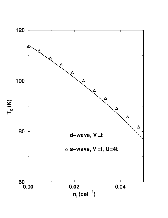
FIG. 6.: The dependence of $T_{c}$ on the concentration $n_{i}$ of in-plane impurities for $T_{J}=90$meV and for the anisotropic electron-phonon coupling model (33) (the same value of $|g|^{2}$ was used as in Figs. (3), (4) and (5)) calculated in the t-matrix approximation, Eq. (12), for the electron-impurity matrix element $V_{i}=t$. The results for d${}_{x^{2}-y^{2}}$-symmetry of the gap are given by the solid line and the results for s-wave symmetry are given by triangles. Note that as $n_{i}$ increases the state with the highest $T_{c}$ crosses over from d${}_{x^{2}-y^{2}}$-symmetry to s-wave symmetry.

FIG. 7.: The isotope coefficient $\alpha=-d\ln T_{c}/d\ln M$ associated with the oxygen optic mode at 500 cm^-1 and the corresponding $T_{c}$ as functions of the interlayer pair tunneling strength $T_{J}=t_{\bot}^{2}/t$. In all cases the on-site Coulomb repulsion $U$ is equal to zero. The results obtained with the isotropic electron-phonon coupling model (32) are labeled as (s-wave isotropic). The results obtained with the anisotropic electron-phonon coupling model (33) are labeled as (s-wave anisotropic) or as (d-wave anisotropic) depending on whether s-wave or d${}_{x^{2}-y^{2}}$-wave symmetry is assumed, respectively. The value of $|g|^{2}$ is the same as in Figs. (3-6) leading to $\lambda=0.48$ in the isotropic case.

- [1] J. M. Wheatly, T. C. Hsu, and P. W. Anderson, Phys. Rev. B 37, 5897 (1988)
- [2] S. Chakravarty, A. Sudbø, P. W. Anderson, and S. Strong, Science 261, 337 (1993).
- [3] A. Sudbø, S. Chakravarty, S. Strong, and P. W. Anderson, Phys. Rev. B 49, 12245 (1994).
- [4] A. Sudbø, Physica C 235-240, 126 (1994).
- [5] A. Sudbø, J. Low Temp. Phys. 97, 403 (1994).
- [6] S. Chakravarty and P. W. Anderson, Phys. Rev. Lett. 72, 3859 (1994).
- [7] D. J. Scalapino, in Superconductivity, edited by R. D. Parks (Marcel Dekker, New York, 1969), Vol. 1, p. 449.
- [8] R. C. Dynes, Solid State Commun. 92, 53 (1994); A. G. Sun, L. M. Paulius, D. A. Gajewski, M. B. Maple, and R. C. Dynes, Phys. Rev. B 50, 3266 (1994).
- [9] S. K. Agrawal, R. Lal, V. P. S. Awans, S. P. Pandey, and A. V. Narlikar, Phys. Rev. B 50, 10265 (1994).
- [10] Y. Fukuzumi, K. Mizuhashi, K. Takenaka, and S. Uchida, Phys. Rev. Lett. 76, 684 (1996).
- [11] S. K. Tolpygo, J. -Y. Lin, M. Gurvitch, S. Y. Hou, and J. M. Phillips, Phys. Rev. B 53, 12454 (1996).
- [12] R. J. Radtke, K. Levin, H. -B. Schüttler, and M. R. Norman, Phys. Rev. B 48, 653 (1993).
- [13] P. Monthoux and D. Pines, Phys. Rev. B 49, 4261 (1994).
- [14] J. Song and J. F. Annett, Phys. Rev. B 51, 3840 (1995); Erratum Phys. Rev. B 52 6930 (1995).
- [15] O. K. Andersen, A. I. Liechtenstein, O. Jepsen, and F. Paulsen, J. Phys. Chem. Solids 56, 1573 (1996).
- [16] J. R. Schrieffer, Theory of Superconductivity (Benjamin, New York, 1964).
- [17] P. B. Allen and B. Mitrović, in Solid State Physics, edited by H. Ehrenreich, F. Seitz, D. Turnbull (Academic, New York, 1982), Vol. 37, p. 1.
- [18] For details see, for example, V. N. Kostur and B. Mitrović, Phys. Rev. B 50, 12774 (1994), ibid. 51, 6064 (1995) and the references therein.
- [19] For details see, for example, T. Höhn and B. Mitrović, Z. Phys. B 93, 173 (1994) and the references therein.
- [20] A. A. Abrikosov, L. P. Gor’kov, I. Ye. Dzyaloshinsky, Quantum Field Theoretical Methods in Statistical Physics, (Pergamon, New York, 1965).
- [21] G. Lehmann and M. Taut, phys. stat. sol. (b) 54, 469 (1972).
- [22] W. Gentzsch, Vectorization of Computer Programs with Applications to Computational Fluid Dynamics (Vieweg, Braunschweig, 1984), pp. 120-121.
- [23] J. W. Serene and D. W. Hess, Phys. Rev. B 44, 3391 (1991).
- [24] Y. Bang, Phys. Rev. B 52, 1279 (1995).
- [25] J. P. Frank, in Physical Properties of High Temperature Superconductors IV, edited by D. M. Ginsberg (World Scientific, Singapore, 1994) p. 189, and the references therein.
- [26] J. H. Nickel, D. E. Morris, and J. W. Ager III, Phys. Rev. Lett. 70, 81 (1993).