Towards a Microscopic Theory for Metallic Heavy-Fermion Point Contacts

Abstract

The bias-dependent resistance $R(V)$ of NS-junctions is calculated using the Keldysh formalism in all orders of the transfer matrix element. We present a compact and simple formula for the Andreev current, that results from the coupling of electrons and holes on the normal side via the anomalous Green’s function on the superconducting side. Using simple BCS Nambu-Green’s functions the well known Blonder-Tinkam-Klapwijk theory can be recovered. Incorporating the energy-dependent quasi-particle lifetime of the heavy fermions strongly reduces the Andreev-reflection signal.

I Introduction

Point-contact spectroscopy (PCS) has been used to study the superconducting (SC) properties of heavy-fermion (HF) compounds, see e.g. Refs.  [1, 2, 3]. The symmetry of the SC order parameter in HF compounds is still not known, and it was hoped that PCS is a useful tool to help clarify this question.

Usually, the SC anomalies of point contacts between HFSC and normal metals have been interpreted in terms of Andreev reflection (AR). But the observed spectra deviate significantly from that predicted by the simple quasi-classical BTK model [7]. For example, the doubling of the electrical current due to AR at a bias voltage $|\text{e}V|=\Delta$ is missing. In recent experiments on UPt₃ [3] and URu₂Si₂ [4] (that are good candidates for being performed in the ballistic limit as claimed by the authors) the size of the SC anomaly amounts to a small fraction of the total signal. We present here a microscopic approach using the Keldysh non-equilibrium method. It incorporates the strongly energy-dependent lifetime in HF compounds, that is also responsible for the large $A$ coefficient of the electrical resistivity at temperatures $T\ll T^{*}$, the lattice Kondo temperature. For vanishing self-energy the BTK result is recovered.

II Theory

We use a simplified model to describe a NS-junction. Let us assume the left side of the junction is described by the Hamiltonian $H_{L}$, the right by $H_{R}$, and the solution of both is known in terms of the one-particle equilibrium Green’s function. The two leads are coupled by a tunnel Hamiltonian [5, 6]

$$H_{T} = \sum_{<L,R>}(T_{L,R}c^{\dagger}_{L\sigma}c_{R\sigma}+h.c.)\;\;.$$ (1)

The applied bias voltage translates into a step-like chemical potential at the junction with the potential difference $\text{e}V$. Hereby the assumption of a ballistic point contact enters the theory. For a diffusive or thermal junction, the spatial dependence of the chemical potential has to be determined self-consistently. The total current

$$I(\tau)=\frac{e}{ih}\sum_{L,R}\mbox{Tr}\left[\tau_{3}\left(\underline{\underline{t}}\;\underline{\underline{G}}_{RL}^{+}(\tau,\tau)-\underline{\underline{t}}^{\dagger}\;\underline{\underline{G}}_{LR}^{+}(\tau,\tau)\right)\right]\;$$ (2)

is in general time-dependent. We introduce the Keldysh Nambu $2\times 2$ occupational Green’s function

$$\underline{\underline{G}}_{LR}^{+}(\tau,\tau^{\prime})=i\left(\begin{array}[]{cc}\ll c^{\dagger}_{L\uparrow}(\tau)c_{R\uparrow}(\tau^{\prime})\gg&\ll c^{\dagger}_{L\uparrow}(\tau)\;c^{\dagger}_{R\downarrow}(\tau^{\prime})\gg\\ \ll c_{L\downarrow}(\tau)\;c_{R\uparrow}(\tau^{\prime})\gg&\ll c_{L\downarrow}(\tau)\;c^{\dagger}_{R\downarrow}(\tau^{\prime})\gg\end{array}\right)$$ (3)

with

$$\underline{\underline{t}}=\left(\begin{array}[]{cc}Te^{i\phi_{0}}&0\\ 0&-Te^{-i\phi_{0}}\end{array}\right)=\left(\begin{array}[]{cc}t_{1}&0\\ 0&-t_{1}^{\star}\end{array}\right)\;\;\;.$$ (4)

In this Nambu representation the hopping matrix element picks up a time-dependent phase difference $\phi(\tau)=\phi_{0}+\tau\omega_{0}/2$ between the two leads, with $\omega_{0}=2\text{e}V/\hbar$.

The current can be decomposed in a Fourier series of multiples of the fundamental frequency $\omega_{0}$: $I(\tau)=\sum_{n}I_{n}\exp(i\tau n\omega_{0})$ necessary for the proper description of a AC Josephson current in SS-junction. In a NS-junction, however, all but the $I_{0}$ component vanish since only $|T|^{2}$ enters in this case. Applying the Keldysh formalism developed for the tunneling theory [6] yields the equations of motion in frequency space

$$\underline{\underline{G}}^{r}_{RL}(\omega) = \underline{\underline{g}}^{r}_{R}(\omega)\underline{\underline{t}}^{\dagger}\;\underline{\underline{G}}^{r}_{L}(\omega)=\underline{\underline{G}}^{r}_{R}(\omega)\;\underline{\underline{t}}^{\dagger}\;\underline{\underline{g}}^{r}_{L}(\omega)$$ (5)

$$\underline{\underline{G}}^{+}_{RL}(\omega) = \underline{\underline{g}}^{+}_{R}(\omega)\;\underline{\underline{t}}\;\underline{\underline{G}}^{a}_{L}(\omega)+\underline{\underline{g}}^{r}_{R}(\omega)\;\underline{\underline{t}}\;\underline{\underline{G}}^{+}_{L}(\omega)$$ (6)

which can be solved, omitting the frequency argument and using

$$\underline{\underline{G}}_{L}^{r} = \underline{\underline{g}}_{L}^{r}+\underline{\underline{g}}_{L}^{r}\;\underline{\underline{\tilde{g}}}_{R}^{r}\;\underline{\underline{G}}_{L}^{r}\;\;\Longrightarrow$$ (7)

$$\underline{\underline{G}}_{L}^{r} = \frac{1}{1-\underline{\underline{g}}_{L}^{r}\;\underline{\underline{\tilde{g}}}_{R}^{r}}\underline{\underline{g}}_{L}^{r}\;\mbox{and}\;\underline{\underline{G}}_{L}^{a}=\underline{\underline{g}}_{L}^{a}\frac{1}{1-\underline{\underline{\tilde{g}}}_{R}^{a}\;\underline{\underline{g}}_{L}^{a}}\;\;,$$ (8)

where the two hopping matrix elements have been absorbed into the renormalized normal-state propagator $\underline{\underline{\tilde{g}}}_{R}(\omega)\equiv|T|^{2}\;\underline{\underline{g}}_{R}(\omega)$ on the right side (R). The left side (L) becomes SC. The denominator indicates the re-summation of tunneling processes in infinite order.

The occupational-components are more complicated:

$$\underline{\underline{G}}_{L}^{\pm} = \frac{1}{1-\underline{\underline{g}}_{L}^{r}\;\underline{\underline{\tilde{g}}}_{R}^{r}}\left[\underline{\underline{g}}_{L}^{\pm}+\underline{\underline{g}}_{L}^{r}\underline{\underline{\tilde{g}}}_{R}^{\pm}\underline{\underline{g}}_{L}^{a}\right]\;\frac{1}{1-\underline{\underline{\tilde{g}}}_{R}^{a}\;\underline{\underline{g}}_{L}^{a}}\;\;.$$ (9)

Here $g$ denotes the equilibrium advanced (a), retarded (r), and occupational ($\pm$) Green’s functions in absence of $H_{T}$, $G$ the fully renormalized non-equilibrium Green’s functions. Using Eqs. (6)-(9), the notation $e(\omega)$ for an electron, $h(\omega)$ for a hole, and $f(\omega)$ for the anomalous Nambu Green’s function component, the total DC current $I(V,t=0)$ of Eq.(2) decomposes into a quasi-particle current

$$I_{QP} = \frac{2e}{h}\sum_{<L,R>}\int\limits_{-\infty}^{\infty}\;d\omega\frac{T^{2}}{|Det[1-\underline{\underline{g}}_{L}^{r}\;\underline{\underline{\tilde{g}}}_{R}^{r}]|^{2}}$$ (13)

$$\left[|1-T^{2}h_{R}^{a}h_{L}^{a}|^{2}(e_{R}^{+}e_{L}^{-}-e_{R}^{-}e_{L}^{+})\right.$$

$$+|T^{2}h_{R}^{a}f_{L}^{a}|^{2}(e_{R}^{+}h_{L}^{-}-e_{R}^{-}h_{L}^{+})$$

$$\left.+2\Re e[(1-T^{2}h_{R}^{a}h_{L}^{a})T^{2}h_{R}^{r}f_{L}^{r}](e_{R}^{+}f_{L}^{-}-e_{R}^{-}f_{L}^{+})\right]$$

and the Andreev current

$$I_{A} = \frac{2e}{h}\sum_{<L,R>}\int\limits_{-\infty}^{\infty}\;d\omega\frac{T^{4}|f_{L}^{r}|^{2}\left[(e_{R}^{+}h_{R}^{-}-e_{R}^{-}h_{R}^{+}\right]}{|Det[1-\underline{\underline{g}}_{L}^{r}\;\underline{\underline{\tilde{g}}}_{R}^{r}]|^{2}}$$ (14)

with ${|Det[1-\underline{\underline{g}}_{L}^{r}\;\underline{\underline{\tilde{g}}}_{R}^{r}]|^{2}}=|(1-T^{2}h_{R}^{r}h_{L}^{r})(1-T^{2}e_{R}^{r}e_{L}^{r})-T^{4}h_{R}^{r}e_{R}^{r}(f_{L}^{r})^{2}|^{2}$.

$I_{QP}$ describes three different processes: an electron on the normal side R couples to an electron, a hole, or to the anomalous GF. The Andreev current couples an electron and a hole on the normal side under the influence of a Cooper pair. Its leading order is $T^{4}$ since it involves two quasi-particles crossing the junction. Note that since we resummed all orders, the hopping $T$ can be tuned continuously from being much smaller than the bandwidth $W$, the tunneling regime, to $\gamma=\pi T\,N_{F}\approx 1$, the metallic PCS regime.

$\sum_{<L,R>}$ denotes two solvable quasi-1d cases:
1. Quantum point contact. The orifice involves only a few lattice sites. Translational invariance is broken and no momentum component is conserved at the boundary. It can be verified that using BCS propagators and identifying $Z^{2}=((1-\gamma^{2})/2\gamma)^{2}$ the BTK theory is reproduced by Eqs. (13) and (14). where $\sum_{<L,R>}$ counts the number of channels. For example, the Andreev current per channel reads

$$I_{A} = \frac{2e}{h}\int\limits_{-\infty}^{\infty}\;d\omega\;T_{A}(\omega)\;\tanh\left[\beta\frac{\omega+V}{2}\right]$$ (15)

$$\left.T_{A}(\omega)\right|_{\omega^{2}<\Delta^{2}} = \frac{4\gamma^{4}}{(1+\gamma^{4})^{2}(1-(\omega/\Delta)^{2})+4\gamma^{4}(\omega/\Delta)^{2}}$$ (16)

$$\left.T_{A}(\omega)\right|_{\omega^{2}>\Delta^{2}} = \frac{4\gamma^{4}}{\left((1+\gamma^{4})\sqrt{\left(\frac{\omega}{\Delta}\right)^{2}-1}+2\gamma^{2}|\omega/\Delta|\right)^{2}}$$ (17)

Obviously the transmission coefficient $T(\omega)$ is continuous at $\omega^{2}=\Delta^{2}$ and its value $\frac{2e}{h}$ is independent of the effective coupling $\gamma$.
2. Two connected half spaces. In this case the momentum parallel to the $\underline{k}_{\parallel}$-plane is conserved. $e(\omega,\underline{k}_{\parallel}),f(\omega,\underline{k}_{\parallel})$ and $f(\omega,\underline{k}_{\parallel})$ become $k_{z}$-summed Green’s functions entering Eq. (13) and (14). The total current is the sum of all independent $\underline{k}_{\parallel}$ contributions. For example, in Eq. 14 an electron is coupled to a hole of the same $\underline{k}_{\parallel}$ which translates into the standard one-particle picture of $\underline{k}\rightarrow-\underline{k}$.

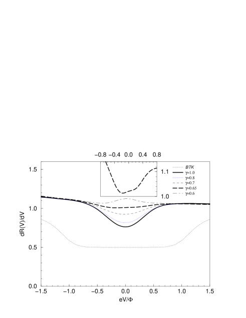
FIG. 1.: Resistance per conductance channel $dV/dI$ vs bias voltage $V$ as function of the dimensionless hopping parameter $\gamma$. Inset: blow-up of the $\gamma=0.65$ curve.

III Application

A microscopic theory of HFSC including quasi-particle lifetime effects is missing up to now. We have used instead the normal state Green’s function for the Anderson lattice

$$\underline{\underline{g}}(z)=\frac{1}{N}\sum_{\underline{k}}\left(\begin{array}[]{c}z-\varepsilon_{\underline{k}}-\frac{V^{2}}{z-T^{\star}}-\Sigma_{c}(z)\;\;,\;\;-\Phi\\ -\Phi\;\;,\;\;z+\varepsilon_{-\underline{k}}-\frac{V^{2}}{z-T^{\star}}-\Sigma^{\ast}_{c}(z)\end{array}\right)^{-1}$$ (18)

with an isotropic order parameter $\Phi=0.1\cdot T^{\ast}$ as a simple, not self-consistent approximation for the SC HF phase where $\Im m\Sigma_{c}(\omega-i\delta)=\frac{1}{2\pi N_{F}}\left(\left(\frac{\pi T}{T^{\star}}\right)^{2}+\left(\frac{\omega}{T^{\star}}\right)^{2}\right)$. This formalism can be easily extended by an anisotropic order parameter $\Phi_{\underline{k}}(i\omega_{n})$ using case 2. Only the conduction electrons contribute to the charge transport since the hybridisation is assumed $k$-independent [8].

The results of Eqs. (13) and (14) are shown in Fig. 1. Ignoring the life-time effects and the hybridisation $V^{2}$ in (18) indeed reproduces the BTK result for $\gamma=1$. But for the HF case a strongly reduced ’V’-shape SC anomaly is found for an ideal metallic point contact ($\gamma=1$). The ’worse’ the contact ($\gamma<1$) the more BTK-like is the shape of an ’ideal’ contact, but its size is strongly reduced at zero bias. Because we have chosen a fixed order parameter $\Phi$ the renormalization due to the strongly reduced quasi-particle spectral weight leads to the ’shrinking’ of the gap. The inset shows a blow-up of the $\gamma=0.65$ curve. This would come close to some of the spectra observed for UPt₃. The asymmetry reflects the asymmetry between the normal electrode (treated by a constant density of states) and the HFSC.

IV Discussion

According to our above calculations the almost flat spectra with small double-minimum structure are accessible only within a very narrow parameter range when coupling is reduced to about $\gamma\approx 0.65$. This could be one of the reasons why those spectra are very hard to detect [3, 4]. Note that even with an isotropic order parameter spectra different from the BTK predictions can be obtained using a energy dependent quasi-particle life-time.

We ought to mention some drawbacks to our approach: The energy-dependence of the quasi-particle lifetime requires a self-consistent determination of the spatial-dependent potential to model contacts in the easily accessible resistance range ($0.3\Omega R<3\Omega$). In an Eliashberg-type of calculation of the SC state the onset of quasi-particle lifetime effects is expected to be shifted self-consistently towards the gap-edges. And we cannot explain the often found enhancement of the ballistic zero-bias resistance.

A recent systematic study on the size of the SC anomalies clearly shows a scaling with the orifice radius rather than with the area [9]. This could indicate that a NNS-junction is seen in most of the experiments with a NS-boundary inside the HF material. Such a scenario would be also favoured in the case of an anisotropic order parameter, since the surface then acts as a pair-braking boundary. A reminiscence of SC is found in the normal-state HF part of the junction, since it is known - or can be easily derived using Eq.(7) - that the non-equilibrium renormalized normal side has a gap at $\omega=0$ in its spectral function induced by the superconductor it is coupled to, which is maintained through large distances (in a pure quasi-particle picture this distance is infinite).

As long as both the experimental and the theoretical situation is not solved completely, PCS is unsuitable as ’smoking gun’-technique to determine the symmetry of the HFSC order parameter.

After finishing our work we became aware, that other authors [10] have also derived the BTK-theory using an Hamiltonian approach to PCS. This work has been supported by the Sonderforschungsbereich 252 Darmstadt-Mainz-Frankfurt, the Deutsche Forschungsgemeinschaft and in parts by the National Science Foundation under Grant No. PHY94-07194. One of us (FBA) likes to thank the ITP, Santa Barbara for its hospitality.

REFERENCES

• [1] A. Nowack et.al., Phys. Rev. B 36, 2436 (1987)
• [2] Y. De Wilde et.al., Phys. Rev. Lett. 72, 2278 (1994)
• [3] G. Goll, C. Bruder, and H. v. Löhneysen, Phys. Rev. B 52, 6801 (1995)
• [4] Yu. G. Naidyuk et.al, Europhysics Lett. 33, 557 (1996)
• [5] J. R. Schrieffer and J. W. Wilkins, Phys. Rev. Lett.  10, 17 (1963)
• [6] C. Caroli et al., J. Phys. C 4, 916 (1972); J. Phys. C 5, 21 (1972)
• [7] G. E. Blonder, M. Tinkham, and T. M. Klapwijk, Phys. Rev. B 25, 4515 (1982)
• [8] D. L. Cox and N. Grewe, Z. Phys. B 71, 321 (1988)
• [9] K. Gloos, S. J. Kim, and G. R. Stewart, J. Low Temp. Phys., 102, 325 (1996); K. Gloos, F. B. Anders, et al., J. Low Temp. Phys., to be publ.
• [10] J. C. Cuevas, A. Martin-Rodero, A. Levy Yeyati 1996, cond-mat/9605023.