On Mean-Field Theory of Quantum Phase Transition in Granular Superconductors

Abstract

In previous work on quantum phase transition in granular superconductors, where mean-field theory was used, an assumption was made that the order parameter as a function of the mean field is a convex up function. Though this is not always the case in phase transitions, this assumption must be verified, what is done in this article.

Quantum phase transition in granular superconductors, modeled as Josephson - junction arrays (JJA) have been a subject of extensive investigations. For a comprehensive review see a book by Šimánek [1]. The picture of the phenomenon is as follows. At the bulk transition temperature $T_{0}$ the magnitude of the order parameter of each superconducting grain becomes nonzero. When the energy of Josephson coupling between grains $E_{J}$ is less than $T_{0}$, thermal fluctuations cause the phases $\theta$ of the order parameter on different grains to be uncorrelated until the temperature is lowered to $T=E_{J}$. When the charging energy $E_{C}$, i.e. the electrostatic energy of a Cooper-pair located on a fixed grain is comparable to $E_{J}$, the zero-point fluctuations of $\theta$ destroy the long-range superconductive order even at zero temperature.

A lot of work have been done to study the phase diagram of the granalular superconductor in ($T/E_{C},E_{J}/E_{C}$) plane [1]. Mostly mean field theory has been used, though recently a renormalization-group study was employed [2]. In previous work, using mean-field theory, an important assumption was made: that the order parameter $<\cos\theta>$ is a convex up function of effective mean field. The aim of this article is to verify this assumption.

Quantum JJA are described by a Hamiltonian [1]:

$$\hat{H}=\sum_{ik}P_{ik}(2e)^{2}\hat{n}_{i}\hat{n}_{k}-\sum_{ik}E_{ik}\cos(\theta_{i}-\theta_{k}).$$ (1)

Here matrix elements $P_{ik}$ are Coulomb interactions and $E_{ik}$ are the Josephson energies between the $i$ and $k$ grains, $\hat{n}_{k}=-id/d\theta_{k}$ is the excess Cooper-pair number operator, conjugate to the phase $\theta_{k}$ of the $k$ grain. While $P_{ik}$ are nonzero for all pairs, $E_{ik}$ are nonzero only for nearest neighbors. In the following we will consider a periodic array of identical grains with identical Josephson junctions between them. This idealization is reasonable when the disorder in Josephson energies and Coulomb interactions is not to big. In opposite case one faces a percolation problem.

The mean-field Hamiltonian in Hartree approximation is obtained by replacing all operators, except two conjugate operators corresponding to chosen grain, by their average values:

$$\hat{H}_{MF}=P(2e)^{2}\hat{n}^{2}-z\mu E_{J}\cos\theta.$$ (2)

Here $z$ is the lattice coordination number; $P=P_{ii}$ is the diagonal element of the potential matrix; $\mu$ is the quantum-statistical and spatial average value of $\cos\theta$; the average value of $\hat{n}$ is zero because of electroneutrality of a sample, and this is why the mean-field Hamiltonian depends on diagonal elements of potential matrix only.

By introducing variables

$$E_{C}=P(2e)^{2};q=z\mu E_{J}/E_{C},$$ (3)

Eq.2 may be rewritten as

$$\hat{H}_{MF}=-E_{C}(d^{2}/d\theta^{2}+q\cos\theta).$$ (4)

We denote the eigenfunctions of the Hamiltonian in Eq.(4) as $\Psi_{n}^{1}$ and $\Psi_{n}^{2}$ and its eigenvalues as $E_{n}^{1}$ and $E_{n}^{2}$. We classify the eigenfunctions by condition $\Psi_{n}^{1}(q=0)=\cos(n\theta)$, $\Psi_{n}^{2}(q=0)=\sin(n\theta)$.

For theory to be self-consistent the value of the order parameter, obtained using the mean-field Hamiltonian should be equal to $\mu$:

$$\mu=\frac{\sum_{n,\alpha}\exp(-E_{n}^{\alpha}/T)<\Psi_{n}^{\alpha}\mid\cos\theta\mid\Psi_{n}^{\alpha}>}{\sum_{n,\alpha}\exp(-E_{n}^{\alpha}/T)}.$$ (5)

From the Feynman-Hellman theorem one obtains

$$<\Psi_{n}\mid\cos\theta\mid\Psi_{n}>=-\frac{1}{E_{C}}dE_{n}/dq.$$ (6)

This means that we just need to calculate $E_{n}^{1}$ and $E_{n}^{2}$ to solve the problem. Hamiltonian in Eq.(4) is similar to the operator of the Mathieu equation [3]:

$$\hat{H}_{Mathieu}=-d^{2}/dx^{2}+2q\cos(2x).$$ (7)

The relation between the eigen-values of (4) and (7) is:

$$E_{n}^{1}(q)=E_{C}\frac{1}{4}a_{2n}(2q);E_{n}^{2}(q)=E_{C}\frac{1}{4}b_{2n}(2q).$$ (8)

In Fig. 1 the order parameter $\mu$, as a function of the mean-field $q$, calculated using Eqs. (5),(6),(8) is plotted. The eigenvalues of Mathieu equation $a_{m}(q)$, $b_{m}(q)$ are calculated using a routine from the IMSL library. $m$’s up to ten have been taken into account. For Fig.1(a) only even order Mathieu functions have been used. This corresponds to taking into account only $2\pi$-periodic $\Psi_{n}$, i.e. those with integer $n$. For Fig.1(b) both even and odd order Mathieu functions have been used, corresponding to $4\pi$-periodic eigenfunctions of (4). Inclusion of $4\pi$-periodic eigenfunctions may serve as an approximation to the continuous spectrum, i.e. to taking into account all $\Psi_{n}$ with real $n$. The latter situation corresponds to the case when the $2\pi$ periodicity is broken by coupling of the Josephson-junction to an environment (for example by normal shunt resistance), which permits a continuous change of the charge on the junction.

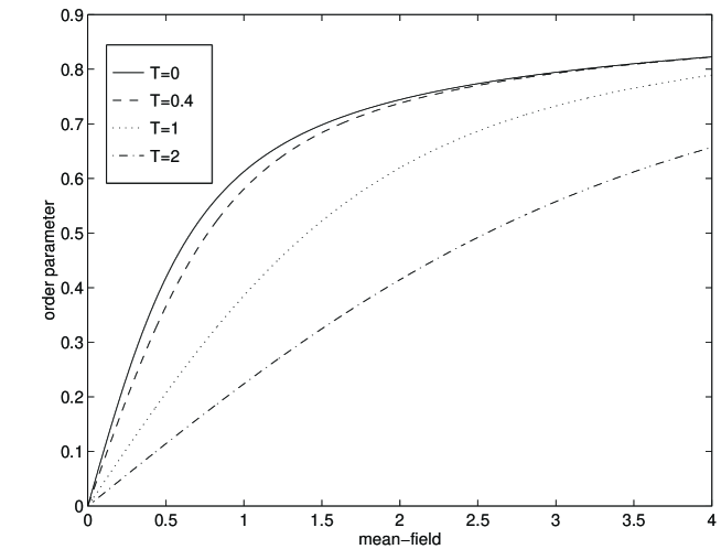
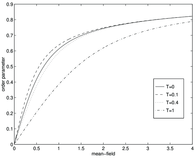
Figure 1: Order parameter $\mu$ as a function of the mean-field $q=z\mu E_{J}/E_{C}$. In (a) only $2\pi$ periodic eigenfunctions of the mean-field Hamiltonian were used. In (b) also $4\pi$ periodic ones were included.

In the previous work only slope of $\mu(q)$ for small $q$ was calculated using either expansion of Mathieu functions for $q\ll 1$ [1], or perturbation series for (4) [4]. Then superconducting transition temperature was calculated from:

$$d\mu(q,T)/dq|_{q=0}=E_{C}/zE_{J},$$ (9)

assuming that $\mu(q)$ is convex up. Fig.1 proves that this assumption is correct for both cases when only $2\pi$ and when also $4\pi$ periodic eigenfunctions are included.

One can consider two types of transition. First is at fixed ratio $E_{J}/E_{C}$ and variable temperature. One can express the order parameter $\mu$ through the mean field $q$ using Eq.3: $\mu=q/(zE_{J}/E_{C})$, and plot this line in Fig.1. The intersection of this line with different curves $\mu(q,T)$ gives the value of the order parameter for each temperature. The second transition is at fixed temperature and variable ratio $E_{J}/E_{C}$. Here one should plot several lines $\mu=q/(zE_{J}/E_{C})$ for different $E_{J}/E_{C}$, and find their intersection with the fixed curve $\mu(q,T)$. As all curves $\mu(q,T)$ in Fig.1 are convex up both mentioned above transitions are continuous.

In Fig.2 a phase diagram of the granular superconductor, calculated using Eq. (9) is presented. In addition the curve for continuous spectrum from Ref.[4] is given. A common feature of phase diagrams, obtained with $4\pi$-periodic eigen-functions and with continuous spectrum is a reentrant transition. Indications for such a transition were observed experimentally, for example, in Ref.[5].

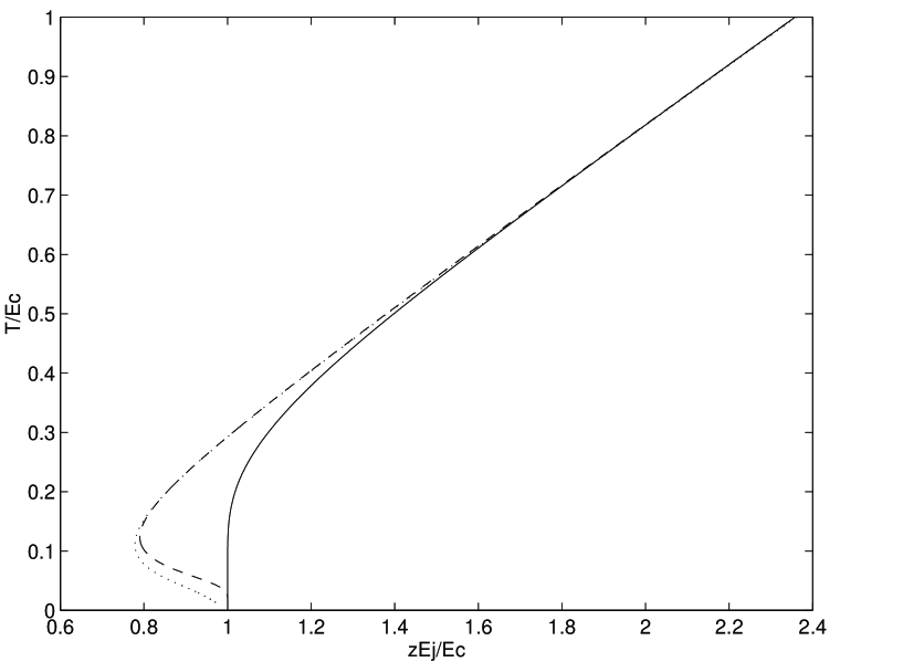
Figure 2: The mean-field phase diagram of a granular superconductor. Solid line is obtained taking into account only $2\pi$-periodic eigenfunctions of (4). Dashed line obtained by including also $4\pi$-periodic ones. Dotted line is from Ref.[4], where a continuum of states was used.

In conclusion, I have verified the assumption, made in earlier work, that the order parameter of granular superconductor is a convex up function of the mean-field, or in other words that the transition is of the second order.

I am grateful to V.K Ignatovich and J.M. Kosterlitz, for useful conversations and to E. Šimánek for correspondence. This work was supported by National Science Foundation Grant No. DMR-9222812.

References

- [1] E. Šimanek, Inhomogeneous Superconductors: Granular and Quantum Effects (Oxford University Press, New York, 1994).
- [2] E. Granato and M.A. Continentino, Phys. Rev. B 48, 15977 (1993).
- [3] N.W. McLachlan, Theory and Applications of Mathieu Functions (Dover Publications, Inc., New York, 1964).
- [4] M.V. Simkin, Phys. Rev. B, 44 (1991) 7074.
- [5] H.S.J. van der Zant, L.J. Geerlings, and J.E. Mooij, Europhys. Lett. 19, 541 (1992).