Soliton Cellular Automata Associated With Crystal Bases

Abstract

We introduce a class of cellular automata associated with crystals of irreducible finite dimensional representations of quantum affine algebras $U^{\prime}_{q}(\hat{\mathfrak{g}}_{n})$. They have solitons labeled by crystals of the smaller algebra $U^{\prime}_{q}(\hat{\mathfrak{g}}_{n-1})$. We prove stable propagation of one soliton for $\hat{\mathfrak{g}}_{n}=A^{(2)}_{2n-1},A^{(2)}_{2n},B^{(1)}_{n},C^{(1)}_{n},D^{(1)}_{n}$ and $D^{(2)}_{n+1}$. For $\hat{\mathfrak{g}}_{n}=C^{(1)}_{n}$, we also prove that the scattering matrices of two solitons coincide with the combinatorial $R$ matrices of $U^{\prime}_{q}(C^{(1)}_{n-1})$-crystals.

1 Introduction

Cellular automata are the dynamical systems in which the dependent variables assigned to a space lattice take discrete values and evolve under a certain rule. They exhibit rich behavior, which have been widely investigated in physics, chemistry, biology and computer sciences [W]. When the space lattice is one dimensional, there are several examples known as the soliton cellular automata [FPS, PF, PAS, PST, TS, T]. They possess analogous features to the solitons in integrable non-linear partial differential equations. For example, some patterns propagate with fixed velocity and they undergo collisions retaining their identity and only changing their phases.

There is a notable progress recently in understanding the integrable structure in the soliton cellular automata. In the papers [TTMS, MSTTT, TNS] it was shown that a class of soliton cellular automata can be derived from the known soliton equations such as Lotka-Volterra and Toda equations through a limiting procedure called ultra-discretization. The method enables one to construct the explicit solutions and the conserved quantities of the former from that of the latter. A key in the ultra-discretization is the identities: $(a,b\in{\mathbb{R}})$

$$\lim_{\epsilon\rightarrow+0}\epsilon\log(e^{\frac{a}{\epsilon}}+e^{\frac{b}{\epsilon}}) = \max(a,b),$$

$$\lim_{\epsilon\rightarrow+0}\epsilon\log(e^{\frac{a}{\epsilon}}\times e^{\frac{b}{\epsilon}}) = a+b.$$

In a sense they change $+$ into $\max$ and $\times$ into $+$. This is a transformation of the continuous operations into piecewise linear ones preserving the distributive law:

$$(A+B)\times C=(A\times C)+(B\times C)\,\rightarrow\,\max(a,b)+c=\max(a+c,b+c).$$

The non-uniqueness of the distributive structure is noted by Schützenberger in combinatorics, where the procedure corresponding to the inverse of the ultra-discretization is called ‘tropical variable change’ [Ki].

There is yet further intriguing aspect in the soliton cellular automata (called ‘box and ball systems’) in [T, TNS]. There the scattering of two solitons is described by the rule which turns out to be identical with the $U_{q}^{\prime}(A^{(1)}_{n})$ combinatorial $R$ matrix [NY] from the crystal base theory. The latter has an origin in the quantum affine algebras at $q=0$, where the representation theory is piecewise linear in a certain sense.

Motivated by these observations we formulate in this paper and [HHIKTT] a class of cellular automata directly in terms of crystals and link the subject to the $1+1$ dimensional quantum integrable systems. The theory of crystals is invented by Kashiwara [Kas] as a representation theory of the quantized Kac-Moody algebras at $q=0$. It is a powerful tool that reduces many essential problems into combinatorial questions on the associated crystals. Irreducible decomposition of tensor products and the Robinson-Schensted-Knuth correspondence are typical such problems [DJM, KN, N]. By connecting the classical and affine crystals, it also explains [KMN1, KMN2] the appearance of the affine Lie algebra characters [DJKMO] in Baxter’s corner transfer matrix method in solvable lattice models [B].

Here we shall introduce a cellular automaton associated with crystals of irreducible finite dimensional representations of quantum affine algebras $U^{\prime}_{q}(\hat{\mathfrak{g}}_{n})$. The basic idea is to regard the time evolution in the automaton as the action of a row-to-row transfer matrix of integrable $U^{\prime}_{q}(\hat{\mathfrak{g}}_{n})$ vertex models at $q=0$. The essential point is to consider the tensor product of crystals not around the ‘anti-ferromagnetic vacuum’ as in [KMN1, KMN2], but rather in the vicinity of the ‘ferromagnetic vacuum’.

Let $B$ be a classical crystal of irreducible finite dimensional representations of the quantum affine algebra $U^{\prime}_{q}(\hat{\mathfrak{g}}_{n})$. It is a finite set having a weight decomposition and equipped with the maps $\tilde{e}_{i},\tilde{f}_{i}:B\rightarrow B\sqcup\{0\}$ and $\varepsilon_{i},\varphi_{i}:B\rightarrow{\mathbb{Z}}_{\geq 0}$ $(i\in\{0,1,\ldots,n\})$ satisfying certain axioms. (cf. Definition 2.1 in [KKM].) For two crystals $B$ and $B^{\prime}$ the tensor products $B^{\prime}\otimes B$ and $B\otimes B^{\prime}$ are again crystals which are canonically isomorphic. The isomorphism $B^{\prime}\otimes B\stackrel{{\scriptstyle\sim}}{{\rightarrow}}B\otimes B^{\prime}$ is called the combinatorial $R$ matrix . Suppose that there are special elements denoted by $1\in B$ and $u_{\natural}\in B^{\prime}$ with the properties

$$({\mathrm{I}}) \quad u_{\natural}\otimes 1\simeq 1\otimes u_{\natural},$$

$$(\mathrm{II}) \quad\text{For any }u\in B^{\prime}\,\text{ there exists }\,k\in{\mathbb{Z}}_{\geq 0}\text{ such that }$$

$$\quad u\otimes\overbrace{1\otimes\cdots\otimes 1}^{k}\simeq b_{1}\otimes\cdots\otimes b_{k}\otimes u_{\natural},\qquad(b_{i}\in B).$$

We take dynamical variables of our automaton from the crystal $B$ and regard their array $\ldots,b^{t}_{-1},b^{t}_{0},b^{t}_{1},\ldots$ at time $t$ as an element of the tensor product of crystals

$$\cdots\otimes b^{t}_{-1}\otimes b^{t}_{0}\otimes b^{t}_{1}\otimes\cdots\in\cdots\otimes B\otimes B\otimes B\otimes\cdots,$$

where we assume the boundary condition $b^{t}_{j}=1\in B$ for $|j|\gg 1$. See Section 2.2 for a precise treatment. The ‘ferromagnetic’ state $\forall b^{t}_{i}=1$ is understood as the vacuum of the automaton. The infinite tensor product with such a boundary condition does not admit a crystal structure. Nevertheless one can make sense of the construction below thanks to the properties (I) and (II). The time evolution is induced by sending $u_{\natural}$ from left to right via the repeated application of the combinatorial $R$ matrix as

$$B^{\prime} \otimes (\cdots \otimes B \otimes B \otimes B \otimes \cdots) \simeq (\cdots \otimes B \otimes B \otimes B \otimes \cdots) \otimes B^{\prime}$$

$$u_{\natural} \otimes (\cdots \otimes b^{t}_{-1} \otimes b^{t}_{0} \otimes b^{t}_{1} \otimes \cdots) \simeq (\cdots \otimes b^{t+1}_{-1} \otimes b^{t+1}_{0} \otimes b^{t+1}_{1} \otimes \cdots) \otimes u_{\natural},$$

which is well-defined as long as the above properties and the boundary conditions are fulfilled. In the language of the quantum inverse scattering method [STF, KS], this is the action of the $q=0$ row-to-row transfer matrix whose auxiliary and quantum spaces are labeled by $B^{\prime}$ and $\cdots\otimes B\otimes B\otimes\cdots$, respectively. Note that the transfer matrix has effectively reduced to the $(u_{\natural},u_{\natural})$-component of the monodromy matrix since its action is considered under the ferromagnetic boundary condition. The fundamental case $\hat{\mathfrak{g}}_{n}=A^{(1)}_{n}$ will be studied in a more general setting in [HHIKTT]. In this paper we concentrate on the other non-exceptional series

$$\hat{\mathfrak{g}}_{n} =A^{(2)}_{2n-1},A^{(2)}_{2n},B^{(1)}_{n},C^{(1)}_{n},D^{(1)}_{n},D^{(2)}_{n+1},$$

with the following choice of crystals:

$$B =B_{1}\ni 1,\quad B^{\prime}=B_{\natural}\ni u_{\natural}.$$

Here $B_{1}$ is the crystal associated with the vector representation of the classical subalgebra of $\hat{\mathfrak{g}}_{n}$ except for $A^{(2)}_{2n}$ and $D^{(2)}_{n+1}$. Their cardinalities are $\sharp B=2n,2n+1,2n+1,2n,2n$ and $2n+2$, respectively. The element $1\in B_{1}$ is the highest weight one . To explain $B_{\natural}$ and $u_{\natural}$, recall the coherent family $\{B_{l}\mid l\in{\mathbb{Z}}_{\geq 1}\}$ of the perfect crystals obtained in [KKM]. It contains the $B_{1}$ as its first member . The $B_{l}$ with higher $l$ corresponds to an $l$-fold symmetric fusion of $B_{1}$. Then $B_{\natural}$ in question is an infinite set corresponding to a certain $l\rightarrow\infty$ limit of $B_{l}$ and $u_{\natural}$ is its highest weight element . We shall call the resulting dynamical system $U^{\prime}_{q}(\hat{\mathfrak{g}}_{n})$ automaton. They are essentially solvable trigonometric vertex models at $q=0$ in the vicinity of the ferromagnetic vacuum. A peculiarity here is the extreme anisotropy with respect to the relevant fusion degrees; $B_{1}$ is the simplest one, while $B^{\prime}=B_{\natural}$ corresponds to an infinite fusion .

Once the automata are constructed the first question will be if they are solitonic. We prove a theorem that

• the $U^{\prime}_{q}(\hat{\mathfrak{g}}_{n})$ automaton has the patterns labeled by the crystals $\{B_{l}\}$ of the algebra $U^{\prime}_{q}(\hat{\mathfrak{g}}_{n-1})$ that propagate stably with velocity $l$.

Computer experiments indicate that they indeed behave like solitons. For instance, the initially separated patterns labeled by the $U^{\prime}_{q}(\hat{\mathfrak{g}}_{n-1})$-crystal elements $b\in B_{l}$ and $c\in B_{k}$ $(l>k)$ undergo a scattering into two patterns labeled again by some $c^{\prime}\in B_{k}$ and $b^{\prime}\in B_{l}$. Let ${\mathcal{S}}:B_{l}\otimes B_{k}\rightarrow B_{k}\otimes B_{l}$ be the two-body scattering matrix of such collisions, namely, ${\mathcal{S}}(b\otimes c)=c^{\prime}\otimes b^{\prime}$. Let ${\mathcal{R}}:B_{l}\otimes B_{k}\rightarrow B_{k}\otimes B_{l}$ denote the combinatorial $R$ matrix of $U^{\prime}_{q}(\hat{\mathfrak{g}}_{n-1})$. Then we prove

• ${\mathcal{S}}={\mathcal{R}}$

for $\hat{\mathfrak{g}}_{n}=C^{(1)}_{n}$ and conjecture it for all the other $\hat{\mathfrak{g}}_{n}$. Similarly the scattering of multi-solitons labeled by $B_{l_{1}},\ldots,B_{l_{N}}$ ($l_{1}>\cdots>l_{N}$) is given by the isomorphism $B_{l_{1}}\otimes\cdots\otimes B_{l_{N}}\simeq B_{l_{N}}\otimes\cdots\otimes B_{l_{1}}$ experimentally. Thus the solitonic nature is guaranteed by the Yang-Baxter equation obeyed by ${\mathcal{S}}={\mathcal{R}}$. A precise formulation of these claims is done through an injection

$$\imath_{l}:U^{\prime}_{q}(\hat{\mathfrak{g}}_{n-1})\text{-crystal }B_{l}\rightarrow(U^{\prime}_{q}(\hat{\mathfrak{g}}_{n})\text{-crystal }B_{1})^{\otimes l},$$

which will be described in Section 3.

Admitting that they are soliton cellular automata, the second question is if there exist classical integrable equations governing them, possibly via the ultra-discretization. Here we only confirm this for $A^{(2)}_{2}$ case by relating the associated automaton to the known $A^{(1)}_{1}$ example [TS]. This observation is due to [HI].

The layout of the paper is as follows. In Section 2 we first explain our construction of the $U^{\prime}_{q}(\hat{\mathfrak{g}}_{n})$ automata concretely along the $\hat{\mathfrak{g}}_{n}=A^{(2)}_{2}$ example. It is valid for any $U^{\prime}_{q}(\hat{\mathfrak{g}}_{n})$ and any finite crystals having the properties (I) and (II). In Section 3, we formulate the theorem and the conjecture for $\hat{\mathfrak{g}}_{n}$ precisely. We sketch a proof of ${\mathcal{S}}={\mathcal{R}}$ for $C^{(1)}_{n}$ case. In principle the idea used in the proof can also be used for the other $\hat{\mathfrak{g}}_{n}$. We will specify $B_{\natural}$ as an infinite set with the actions $\tilde{e}_{i},\tilde{f}_{i}:B_{\natural}\rightarrow B_{\natural}\sqcup\{0\}$ but without the maps $\varepsilon_{i},\varphi_{i}$. In Section 4 concluding remarks are given. Appendix A is devoted to an explanation of what is meant by ‘$B_{\natural}\otimes B_{1}\simeq B_{1}\otimes B_{\natural}$’, which shows up when the infinite set $B_{\natural}$ is substituted into the finite crystal $B^{\prime}$. This is actually abuse of notation meaning an invertible map $R^{\prime}:B_{\natural}\times B_{1}\rightarrow B_{1}\times B_{\natural}$ between the sets. We state a conjecture on a stability of the combinatorial $R$ matrix $B_{l}\otimes B_{1}\simeq B_{1}\otimes B_{l}$ when $l$ gets large, which ensures the well-definedness of the map $R^{\prime}$. It assures that we may regard $B_{\natural}$ as a finite crystal $B_{l}$ with a sufficiently large $l$ to define our automata.

Our construction here and in [HHIKTT] is a crystal interpretation of the $L$-operator approach [HIK] for a $\hat{\mathfrak{g}}_{n}=A^{(1)}_{n}$ case. The $U^{\prime}_{q}(A^{(1)}_{n})$ automaton in this sense coincides with the ones in [TS, T, TNS]. As in the $C^{(1)}_{n}$ case in this paper, the properties stated in the above can actually be proved by means of the crystal theory. The detail will appear elsewhere along with the results on a more general choice of the crystals $B$ and $B^{\prime}$ [HHIKTT].

Acknowledgements   The authors thank K. Hikami, R. Inoue, T. Nakashima, M. Okado, T. Takebe, T. Tokihiro, Z. Tsuboi and Y. Yamada for valuable discussions.

2 $A^{(2)}_{2}$ example

Let us explain our automata concretely along the case $\hat{\mathfrak{g}}_{n}=A^{(2)}_{2}$. This simple example is helpful to gain the idea for the general $\hat{\mathfrak{g}}_{n}$ case treated in the next section.

As a peculiarity in the rank 1 situation, the $U^{\prime}_{q}(A^{(2)}_{2})$ automaton turns out to be an ‘even time sector’ of [TS].

2.1 $A^{(2)}_{2}$ crystals

For $l\in{\mathbb{Z}}_{\geq 1}$ set

$$B_{l}=\{(x,y)\mid x,y\in{\mathbb{Z}}_{\geq 0},\,x+y\leq l\}.$$ (2.1)

The action of the Kashiwara operators ${\tilde{e}}_{i},{\tilde{f}}_{i}(i=0,1):B_{l}\rightarrow B_{l}\sqcup\{0\}$ are given by

$${\tilde{e}}_{0}(x,y) = \begin{cases}(x-1,y)&\text{if $x>y$},\\ (x,y+1)&\text{if $x\leq y$},\end{cases}\quad{\tilde{e}}_{1}(x,y)=(x+1,y-1),$$

$${\tilde{f}}_{0}(x,y) = \begin{cases}(x+1,y)&\text{if $x\geq y$},\\ (x,y-1)&\text{if $x<y$},\end{cases}\quad{\tilde{f}}_{1}(x,y)=(x-1,y+1).$$

In the above, the right hand sides are to be understood as $0$ if they are not in $B_{l}$. Setting $\varepsilon_{i}(b)=\max_{k}\{\tilde{e}_{i}^{k}b\neq 0\mid k\geq 0\}$ and $\varphi_{i}(b)=\max_{k}\{\tilde{f}_{i}^{k}b\neq 0\mid k\geq 0\}$, one has

$$\varepsilon_{0}(b) =l-x-y+2(x-y)_{+},\quad\varepsilon_{1}(b) =y,$$

$$\varphi_{0}(b) =l-x-y+2(y-x)_{+},\quad\varphi_{1}(b) =x,$$

for $b=(x,y)\in B_{l}$. Here the symbol $(\cdot)_{+}$ stands for

$$(x)_{+}=\max(0,x).$$

These results are obtained by extrapolating the $A^{(2)}_{2n}$ result [KKM] to $n=1$. For $l=1$ we use a simpler notation as

$$B=B_{1},\quad 1=(1,0),\,2=(0,0),\,3=(0,1).$$ (2.2)

Given two crystals $B$ and $B^{\prime}$, one can form another crystal (tensor product) $B\otimes B^{\prime}$ [Kas]. The crystal $B_{l}\otimes B_{1}$ is connected and so is $B_{1}\otimes B_{l}$. Calculating the map $B_{l}\otimes B_{1}\rightarrow B_{1}\otimes B_{l}$ commuting with $\tilde{e}_{i}$ and $\tilde{f}_{i}$, one has

Proposition 2.1.

The combinatorial $R$ matrix $B_{l}\otimes B\simeq B\otimes B_{l}$ is given by

$$(x,y)\otimes 1 \simeq \begin{cases}1\otimes(l,0)&\text{if $(x,y)=(l,0)$},\\ 3\otimes(x+1,y-1)&\text{if $x+y=l,\,y\geq 1$},\\ 2\otimes(x+1,y)&\text{if $x+y=l-1$},\\ 1\otimes(x+1,y+1)&\text{otherwise},\end{cases}$$

$$(x,y)\otimes 2 \simeq \begin{cases}1\otimes(l-1,0)&\text{if $(x,y)=(l,0)$},\\ 3\otimes(x,y-1)&\text{if $x+y=l,\,y\geq 1$},\\ 2\otimes(x,y)&\text{otherwise},\end{cases}$$

$$(x,y)\otimes 3 \simeq \begin{cases}3\otimes(0,l)&\text{if $(x,y)=(0,l)$},\\ 2\otimes(0,l)&\text{if $(x,y)=(0,l-1)$},\\ 1\otimes(0,1)&\text{if $(x,y)=(1,0)$},\\ 1\otimes(x-2,y)&\text{if $2\leq x\leq l,\,y=0$},\\ 1\otimes(x,y+2)&\text{if $x=0,\,0\leq y\leq l-2$},\\ 3\otimes(x-1,y-1)&\text{otherwise}.\end{cases}$$

In Section 2.2 we shall use formal $l\rightarrow\infty$ limits of $B_{l}$ and the combinatorial $R$ matrix $B_{l}\otimes B\simeq B\otimes B_{l}$. In the present case the prescription is to simply shift the coordinate $(x,y)$ to $(x-l,y)$ and to consider

$$B_{\natural}=\{(x,y)\mid x\in{\mathbb{Z}}_{\leq 0},y\in{\mathbb{Z}}_{\geq 0},x+y\leq 0\},$$

without specifying a crystal structure. The map $R^{\prime}:B_{\natural}\otimes B\simeq B\otimes B_{\natural}$ in the sense of Appendix A is deduced from Proposition 2.1 by concentrating on those $(x,y)$ in the vicinity of $(0,0)$. Thus it reads

$$(x,y)\otimes 1 \simeq \begin{cases}1\otimes(0,0)&\text{if $(x,y)=(0,0)$},\\ 3\otimes(x+1,y-1)&\text{if $x+y=0,\,y\geq 1$},\\ 2\otimes(x+1,y)&\text{if $x+y=-1$},\\ 1\otimes(x+1,y+1)&\text{otherwise},\end{cases}$$ (2.3)

$$(x,y)\otimes 2 \simeq \begin{cases}1\otimes(-1,0)&\text{if $(x,y)=(0,0)$},\\ 3\otimes(x,y-1)&\text{if $x+y=0,\,y\geq 1$},\\ 2\otimes(x,y)&\text{otherwise},\end{cases}$$ (2.4)

$$(x,y)\otimes 3 \simeq \begin{cases}1\otimes(x-2,y)&\text{if $y=0$},\\ 3\otimes(x-1,y-1)&\text{otherwise}.\end{cases}$$ (2.5)

To depict this in a figure we put ${b\atop b^{\prime}}$ beside the arrow $(x,y)\rightarrow(x^{\prime},y^{\prime})$ to signify the relation

$$R^{\prime}:(x,y)\otimes b\xrightarrow{\sim}b^{\prime}\otimes(x^{\prime},y^{\prime}).$$

We call $b$ and $b^{\prime}$ the upper index and the lower index, respectively. Now (2.3)–(2.5) are summarized in the semi-infinite triangle in Figure 1.

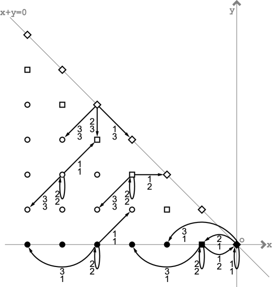
Figure 1:

The Semi-infinite triangle representing $R^{\prime}$. There are 6 different patterns depicted by circles, squares and diagonal squares which are filled or empty.

2.2 Cellular automaton

By applying $B_{\natural}\otimes B\simeq B\otimes B_{\natural}$ successively one has

$$B_{\natural} \otimes \overbrace{B\otimes\cdots\otimes B}^{L} \simeq \overbrace{B\otimes\cdots\otimes B}^{L} \otimes B_{\natural}$$

$$u \otimes b_{i}\otimes\cdots\otimes b_{j} \simeq b^{\prime}_{i}\otimes\cdots\otimes b^{\prime}_{j} \otimes u^{\prime}$$ (2.6)

for any $L\in{\mathbb{Z}}_{\geq 1}$, where $i=-[\frac{L}{2}],j=i+L-1$ . Denote the element $(0,0)\in B_{\natural}$ by $u_{\natural}$. The map $R^{\prime}:B_{\natural}\otimes B\simeq B\otimes B_{\natural}$ (2.3)–(2.5) has the properties (I) and (II) in Section 1. Set

$${\mathcal{P}}=\{b:{\mathbb{Z}}\rightarrow B\mid b_{j}=1\in B\text{ for }|j|\gg 1\}.$$

We shall regard ${\mathcal{P}}$ as a subset of the tensor product which is formally infinite in both directions, i.e.,

$${\mathcal{P}}=\{\cdots\otimes b_{-1}\otimes b_{0}\otimes b_{1}\otimes\cdots\in\cdots\otimes B\otimes B\otimes B\otimes\cdots\mid b_{j}=1\text{ for }|j|\gg 1\}.$$ (2.7)

In the latter picture one should distinguish the elements even though they are the same under translations. For example,

$$\cdots 1\otimes 1\otimes 1\otimes 2\otimes 3\otimes 1\otimes 1\otimes 1\otimes\cdots,$$

$$\cdots 1\otimes 1\otimes 1\otimes 1\otimes 2\otimes 3\otimes 1\otimes 1\otimes\cdots$$

are distinct elements in ${\mathcal{P}}$. The set ${\mathcal{P}}$ (2.7) is not equipped with a crystal structure. Nevertheless the properties (I) and (II) enable us to define an invertible map $T:{\mathcal{P}}\rightarrow{\mathcal{P}}$ that formally corresponds to an $L\rightarrow\infty$ limit of (2.6). To describe it precisely, note that any element in ${\mathcal{P}}$ has the form

$$p=\cdots\otimes 1\otimes 1\otimes b_{i}\otimes\cdots\otimes b_{j}\otimes 1\otimes 1\otimes\cdots\quad(i\leq j),$$ (2.8)

where $b_{i},b_{i+1},\ldots,b_{j}\in B$. Owing to the properties (I) and (II) there exists $k_{0}\in{\mathbb{Z}}_{\geq 0}$ such that

$$u_{\natural}\otimes b_{i}\otimes\cdots\otimes b_{j}\otimes\overbrace{1\otimes\cdots\otimes 1}^{k}\simeq b^{\prime}_{i}\otimes\cdots\otimes b^{\prime}_{j}\otimes b^{\prime}_{j+1}\otimes\cdots\otimes b^{\prime}_{j+k}\otimes u_{\natural}$$

for all $k\geq k_{0}$. Then $T(p)\in{\mathcal{P}}$ is defined by

$$T(p)=\cdots\otimes 1\otimes 1\otimes b^{\prime}_{i}\otimes\cdots\otimes b^{\prime}_{j}\otimes b^{\prime}_{j+1}\otimes\cdots\otimes b^{\prime}_{j+k}\otimes 1\otimes 1\otimes\cdots,$$

which is $k$-independent as long as $k\geq k_{0}$. The inverse $T^{-1}$ can be described similarly.

The map $T$ plays the role of the ‘time evolution’ operator. It is a $q=0$ analogue of the row-to-row transfer matrix of a solvable lattice model in the vicinity of the ferromagnetic vacuum.

Given $p\in{\mathcal{P}}$ in (2.8) define $u_{m}\in B_{\natural}$ for all $m\in{\mathbb{Z}}$ by the recursion relation and the boundary condition

$$u_{m-1}\otimes b_{m} \simeq b^{\prime}_{m}\otimes u_{m}\quad\text{ for all }\,m\in{\mathbb{Z}},$$

$$u_{m} = u_{\natural}\quad\qquad\text{ for }\,m\leq i-1.$$

Plainly, $u_{\natural}\otimes(\cdots\otimes b_{m-1}\otimes b_{m}\otimes b_{m+1}\otimes\cdots)\simeq\cdots\otimes b^{\prime}_{m-1}\otimes b^{\prime}_{m}\otimes u_{m}\otimes b_{m+1}\otimes\cdots$. Due to the properties (I) and (II) the sequence $u_{m},u_{m+1},\ldots$ tends to $u_{\natural}=(0,0)\in B_{\natural}$. In this way any element $p\in{\mathcal{P}}$ specifies a trajectory $\{u_{m}\}_{m=-\infty}^{\infty}$ in the semi-infinite triangle (Figure 1) that starts at the origin $(0,0)$ and returns to it finally. This picture is useful in calculating $T(p)$. Namely, the trajectory is determined by following the arrows with the upper indices $\ldots,b_{m-1},b_{m},b_{m+1},\ldots$ appearing in $p=\cdots\otimes b_{m-1}\otimes b_{m}\otimes b_{m+1}\otimes\cdots$. Then $T(p)$ is constructed by tracing their lower indices as $T(p)=\cdots\otimes b^{\prime}_{m-1}\otimes b^{\prime}_{m}\otimes b^{\prime}_{m+1}\otimes\cdots$.

For $p=\cdots\otimes b_{j}\otimes b_{j+1}\otimes\cdots\in{\mathcal{P}}$ and $t\in{\mathbb{Z}}$ define $b^{t}_{j}\in B$ by $T^{t}(p)=\cdots\otimes b^{t}_{j}\otimes b^{t}_{j+1}\otimes\cdots$. Then the time evolution of the cellular automaton is displayed with the arrays

$$\begin{array}[]{ccccccc}\ldots&b^{0}_{-2}&b^{0}_{-1}&b^{0}_{0}&b^{0}_{1}&b^{0}_{2}&\ldots\\ \ldots&b^{1}_{-2}&b^{1}_{-1}&b^{1}_{0}&b^{1}_{1}&b^{1}_{2}&\ldots\\ \ldots&b^{2}_{-2}&b^{2}_{-1}&b^{2}_{0}&b^{2}_{1}&b^{2}_{2}&\ldots\\ \end{array}$$

Let us present a few examples.

Example 2.2.

t=0 : $\cdots$11233311111111111111111111111$\cdots$

t=1 : $\cdots$11111111123331111111111111111$\cdots$

t=2 : $\cdots$11111111111111112333111111111$\cdots$

t=3 : $\cdots$11111111111111111111111233311$\cdots$

Example 2.3.

t=0 : $\cdots$11333311111111111111111111111111$\cdots$

t=1 : $\cdots$11111111113333111111111111111111$\cdots$

t=2 : $\cdots$11111111111111111133331111111111$\cdots$

t=3 : $\cdots$11111111111111111111111111333311$\cdots$

Example 2.4.

t=0 : $\cdots$1133311111123111111111111111111111$\cdots$

t=1 : $\cdots$1111111133311123111111111111111111$\cdots$

t=2 : $\cdots$1111111111111133123311111111111111$\cdots$

t=3 : $\cdots$1111111111111111123111133311111111$\cdots$

t=4 : $\cdots$1111111111111111111123111111133311$\cdots$

Example 2.5.

t=0 : $\cdots$11233111331111111111111211111111111111111111111$\cdots$

t=1 : $\cdots$11111112331133111111111121111111111111111111111$\cdots$

t=2 : $\cdots$11111111111133112331111112111111111111111111111$\cdots$

t=3 : $\cdots$11111111111111113311123311211111111111111111111$\cdots$

t=4 : $\cdots$11111111111111111111331111223311111111111111111$\cdots$

t=5 : $\cdots$11111111111111111111111133121111233111111111111$\cdots$

t=6 : $\cdots$11111111111111111111111111121331111112331111111$\cdots$

t=7 : $\cdots$11111111111111111111111111112111133111111123311$\cdots$

Example 2.6.

t=0 : $\cdots$11233111111133111121111111111111111111111111111$\cdots$

t=1 : $\cdots$11111112331111113312111111111111111111111111111$\cdots$

t=2 : $\cdots$11111111111123311112133111111111111111111111111$\cdots$

t=3 : $\cdots$11111111111111111233211113311111111111111111111$\cdots$

t=4 : $\cdots$11111111111111111111211233111331111111111111111$\cdots$

t=5 : $\cdots$11111111111111111111121111112331133111111111111$\cdots$

t=6 : $\cdots$11111111111111111111112111111111133112331111111$\cdots$

t=7 : $\cdots$11111111111111111111111211111111111113311123311$\cdots$

The last two show the independence of the order of collisions. These examples suggest that the following patterns are stable ($Q\in{\mathbb{Z}}_{\geq 1},R=0,1$):

$$\cdots\otimes \overbrace{2\otimes 3\otimes\cdots\otimes 3}^{Q} \otimes\cdots \quad R=1,$$

$$\cdots\otimes \overbrace{3\otimes 3\otimes\cdots\otimes 3}^{Q} \otimes\cdots \quad R=0.$$

The both patterns should not be followed by $3$. The former pattern can be preceded by any element in $B$ while the latter should only be preceded by $1$. $Q$ is the size of the soliton and $R$ is the number of occurrences of $2$ in its front. They move to the right with the velocity $2Q-R$ when separated sufficiently. These features are consistent with $\hat{\mathfrak{g}}_{n}=A^{(2)}_{2}$ case of Theorem 3.1. See also Section 3.2.

In fact the $U^{\prime}_{q}(A^{(2)}_{2})$ automaton described above can be interpreted [HI] as an ‘even time sector’ of the automaton in [TS]. Replace the array of $\{1,2,3\}$ by that of $\{1,2\}$ with double length via the rule $1\rightarrow 11,2\rightarrow 12$ and $3\rightarrow 22$. In the resulting array, play the ‘box and ball game’ as in [TS]. Namely, we regard the array as a sequence of cells which contains a ball or not according to the array variable is $2$ or $1$, respectively. In each time step, we move each ball once to the nearest right empty box starting from the leftmost ball. Then the 2 time steps in the box and ball system yield the 1 time step in our $U^{\prime}_{q}(A^{(2)}_{2})$ automaton.

In terms of crystals, this can be explained as follows. First, the box and ball game in [TS] is known [HHIKTT] to be equivalent to the $U^{\prime}_{q}(A^{(1)}_{1})$ automaton. Let

$$\hat{B}_{k}=\{m_{1}\ldots m_{k}\mid m_{i}\in\{1,2\},m_{1}\leq\cdots\leq m_{k}\}$$

denote the $U^{\prime}_{q}(A^{(1)}_{1})$-crystal corresponding to the $k$-fold symmetric tensor representation. (We have omitted the frame of the usual semistandard tableaux.) Consider the maps $h_{\natural}$ and $h_{1}$ defined by

$$h_{\natural}: \quad B_{\natural}\quad\longrightarrow\quad\qquad\quad\;\hat{B}_{k}\otimes\hat{B}_{k}\quad(k\gg 1)$$

$$(x,y)\quad\mapsto\quad\overbrace{1\ldots 1}^{k-2y}\overbrace{2\ldots 2}^{2y}\otimes\overbrace{1\ldots 1}^{k+x+y}\overbrace{2\ldots 2}^{-x-y},$$

$$h_{1}: \quad B_{1}\longrightarrow\hat{B}_{1}\otimes\hat{B}_{1}$$

$$\quad 1\quad\mapsto\quad 1\otimes 1$$

$$\quad 2\quad\mapsto\quad 1\otimes 2$$

$$\quad 3\quad\mapsto\quad 2\otimes 2.$$

Then for $k$ large enough, we have the commutative diagram:

$$\begin{CD}B_{\natural}\otimes B_{1}@>{h_{\natural}\otimes h_{1}}>{}>\hat{B}_{k}\otimes\hat{B}_{k}\otimes\hat{B}_{1}\otimes\hat{B}_{1}\\ @V{R^{\prime}}V{}V@V{}V{}V\\ B_{1}\otimes B_{\natural}@>{h_{1}\otimes h_{\natural}}>{}>\hat{B}_{1}\otimes\hat{B}_{1}\otimes\hat{B}_{k}\otimes\hat{B}_{k},\end{CD}$$

where the down arrow in the right column is the crystal isomorphism. This asserts that the square of the $T$ in the $U^{\prime}_{q}(A^{(1)}_{1})$ automaton coincides with the $T$ of the $U^{\prime}_{q}(A^{(2)}_{2})$ automaton.

3 $U^{\prime}_{q}(\hat{\mathfrak{g}}_{n})$ automaton

3.1 Theorem and conjecture

Let us proceed to the $U^{\prime}_{q}(\hat{\mathfrak{g}}_{n})$ automata for $\hat{\mathfrak{g}}_{n}=A^{(2)}_{2n-1}\;(n\geq 3),A^{(2)}_{2n}\;(n\geq 1),B^{(1)}_{n}\;(n\geq 3),C^{(1)}_{n}\;(n\geq 2),D^{(1)}_{n}\;(n\geq 4)$ and $D^{(2)}_{n+1}\;(n\geq 2)$. Our aim here is to formulate the theorem and the conjecture stated in Section 1 precisely. In principle construction of the automata is the same as the $A^{(2)}_{2}$ case explained in Section 2.2. The time evolution operator $T$ is constructed from the invertible map $R^{\prime}:B_{\natural}\otimes B_{1}\rightarrow B_{1}\otimes B_{\natural}$ in the sense of Appendix A. However its analytic form like (2.3)–(2.5) is yet unknown for general $\hat{\mathfrak{g}}_{n}$ . Thus we have generated the combinatorial $R$ matrix $R:B_{l}\otimes B_{1}\simeq B_{1}\otimes B_{l}$ directly by computer, and investigated the automata associated with $R$ instead of $R^{\prime}$ for several large $l$. Consistently with Conjecture A.1, their behaviour becomes stable when $l$ gets large, yielding our automata associated with $R^{\prime}$.

What we present in Section 3.2 is the list of the data $B_{l},B_{\natural},u_{\natural}$ and $\imath_{l}$ for each $\hat{\mathfrak{g}}_{n}$. We change the notation slightly from Section 1 and 2, representing elements in $B=B_{1}$ with symbols inside a box or $\phi$. For example the special (highest weight) element $1\in B_{1}$ in the properties (I)–(II) is denoted by $1$ . Consequently a state of the automata at each time is represented by an element in

$${\mathcal{P}}=\{b:{\mathbb{Z}}\rightarrow B\mid b_{j}=\framebox{\parbox[c][6.5pt][b]{4.5pt}{$1$}}\in B\text{ for }|j|\gg 1\},$$

which is also interpreted as

$${\mathcal{P}}=\{\cdots\otimes b_{-1}\otimes b_{0}\otimes b_{1}\otimes\cdots\in\cdots\otimes B\otimes B\otimes B\otimes\cdots\mid b_{j}=\framebox{\parbox[c][6.5pt][b]{4.5pt}{$1$}}\text{ for }|j|\gg 1\}.$$

We let $T:{\mathcal{P}}\rightarrow{\mathcal{P}}$ denote the time evolution operator as in Section 2.2. The essential data is the injection

$$\imath_{l}:U^{\prime}_{q}(\hat{\mathfrak{g}}_{n-1})\text{-crystal }B_{l}\rightarrow(U^{\prime}_{q}(\hat{\mathfrak{g}}_{n})\text{-crystal }B_{1})^{\otimes l},$$

which will be utilized to label solitons in the $U^{\prime}_{q}(\hat{\mathfrak{g}}_{n})$ automata in terms of elements of the $U^{\prime}_{q}(\hat{\mathfrak{g}}_{n-1})$-crystal $B_{l}$.

First we claim stable propagation of the 1-soliton as

Theorem 3.1.

For any $l\in{\mathbb{Z}}_{\geq 1}$ and $b\in U^{\prime}_{q}(\hat{\mathfrak{g}}_{n-1})\text{-crystal }B_{l}$, the time evolution map $T$ acts on the state

$$\cdots\otimes\framebox{\parbox[c][6.5pt][b]{4.5pt}{$1$}}\otimes\framebox{\parbox[c][6.5pt][b]{4.5pt}{$1$}}\otimes\imath_{l}(b)\otimes\framebox{\parbox[c][6.5pt][b]{4.5pt}{$1$}}\otimes\framebox{\parbox[c][6.5pt][b]{4.5pt}{$1$}}\otimes\cdots$$

as the overall translation to the right by $l$ slots.

Thus $l$ is the velocity of the soliton. Even when $n$ is the minimal possible value for $\hat{\mathfrak{g}}_{n}$, Theorem 3.1 makes sense if $\imath_{l}$ and $B_{l}$ for ‘$U^{\prime}_{q}(\hat{\mathfrak{g}}_{n-1})$’ are interpreted appropriately by an extrapolation of the data given in Section 3.2. For example, the solitons for $\hat{\mathfrak{g}}_{n}=A^{(2)}_{2}$ case argued in Section 2.2 agree with those coming from ‘$U^{\prime}_{q}(A^{(2)}_{0})$-crystal $B_{l}$’ in such a sense. The proof is given in Section 3.3. For scattering of two solitons we have

Theorem 3.2.

Let $\hat{\mathfrak{g}}_{n}=C^{(1)}_{n}\,(n\geq 3)$. For fixed positive integers $l>k$, let $B_{l}\otimes B_{k}\ni b_{1}\otimes b_{2}\simeq c_{2}\otimes c_{1}\in B_{k}\otimes B_{l}$ be an isomorphism under the combinatorial $R$ matrix of the $U^{\prime}_{q}(\hat{\mathfrak{g}}_{n-1})$-crystals . Then for $m\gg l$, there exists $t_{0}>0$ such that for any $t\geq t_{0}$ and some $m^{\prime}$

$$T^{t} : \cdots\otimes\framebox{\parbox[c][6.5pt][b]{4.5pt}{$1$}}\otimes\framebox{\parbox[c][6.5pt][b]{4.5pt}{$1$}}\otimes\imath_{l}(b_{1})\otimes\framebox{\parbox[c][6.5pt][b]{4.5pt}{$1$}}^{\,\otimes m}\otimes\imath_{k}(b_{2})\otimes\framebox{\parbox[c][6.5pt][b]{4.5pt}{$1$}}\otimes\framebox{\parbox[c][6.5pt][b]{4.5pt}{$1$}}\otimes\framebox{\parbox[c][6.5pt][b]{4.5pt}{$1$}}\cdots\cdots\cdots$$

$$\mapsto \cdots\cdots\otimes\framebox{\parbox[c][6.5pt][b]{4.5pt}{$1$}}\otimes\framebox{\parbox[c][6.5pt][b]{4.5pt}{$1$}}\otimes\framebox{\parbox[c][6.5pt][b]{4.5pt}{$1$}}\otimes\imath_{k}(c_{2})\otimes\framebox{\parbox[c][6.5pt][b]{4.5pt}{$1$}}^{\,\otimes m^{\prime}}\otimes\imath_{l}(c_{1})\otimes\framebox{\parbox[c][6.5pt][b]{4.5pt}{$1$}}\otimes\framebox{\parbox[c][6.5pt][b]{4.5pt}{$1$}}\otimes\cdots.$$

In other words, we have the combinatorial $R$ matrix as the scattering matrix of the ultra-discrete solitons. Compared with $\imath_{l}(b_{1})$, $\imath_{k}(c_{2})$ is shifted to the right, but we do not concern the precise distance. A sketch of a proof of Theorem 3.2 will be given in Section 3.4.

In fact we have a conjecture on $N$-soliton case for general $\hat{\mathfrak{g}}_{n}$.

Conjecture 3.3.

Let $N\in{\mathbb{Z}}_{\geq 2}$. Fix positive integers $k_{1},\ldots,k_{N}$ ($k_{1}>\cdots>k_{N}$) and the elements $b_{i}\in B_{k_{i}}\,(i=1,\ldots,N)$ of the $U^{\prime}_{q}(\hat{\mathfrak{g}}_{n-1})$-crystals. Define $c_{i}\in B_{k_{i}}$ by $b_{1}\otimes\cdots\otimes b_{N}\simeq c_{N}\otimes\cdots\otimes c_{1}$ under the isomorphism $B_{k_{1}}\otimes B_{k_{2}}\otimes\cdots\otimes B_{k_{N}}\simeq B_{k_{N}}\otimes\cdots\otimes B_{k_{2}}\otimes B_{k_{1}}$. For $m_{1},\ldots,m_{N-1}\gg k_{1}$, there exists $t_{0}>0$ such that for any $t\geq t_{0}$,

$$T^{t} : \cdots\otimes\framebox{\parbox[c][6.5pt][b]{4.5pt}{$1$}}\otimes\imath_{k_{1}}(b_{1})\otimes\framebox{\parbox[c][6.5pt][b]{4.5pt}{$1$}}^{\,\otimes m_{1}}\otimes\cdots\otimes\framebox{\parbox[c][6.5pt][b]{4.5pt}{$1$}}^{\,\otimes m_{N-1}}\otimes\imath_{k_{N}}(b_{N})\otimes\framebox{\parbox[c][6.5pt][b]{4.5pt}{$1$}}\otimes\cdots$$

$$\mapsto \quad\cdots\otimes\framebox{\parbox[c][6.5pt][b]{4.5pt}{$1$}}\otimes\imath_{k_{N}}(c_{N})\otimes\framebox{\parbox[c][6.5pt][b]{4.5pt}{$1$}}^{\,\otimes m^{\prime}_{1}}\otimes\cdots\otimes\framebox{\parbox[c][6.5pt][b]{4.5pt}{$1$}}^{\,\otimes m^{\prime}_{N-1}}\otimes\imath_{k_{1}}(c_{1})\otimes\framebox{\parbox[c][6.5pt][b]{4.5pt}{$1$}}\otimes\cdots,$$

holds for some $m^{\prime}_{1},\ldots,m^{\prime}_{N-1}$.

In particular, $c_{1},\ldots,c_{N}$ do not depend on $m_{i}$’s (i.e.,the order of collisions) as long as $m_{i}\gg k_{1}$. Again we do not concern the precise distance between $\imath_{k_{1}}(b_{1})$ and $\imath_{k_{N}}(c_{N})$ in the above.

The rank $n$ in Conjecture 3.3 should be taken greater than the minimal possible values, i.e., $A^{(2)}_{2n-1}\;(n\geq 4),A^{(2)}_{2n}\;(n\geq 2),B^{(1)}_{n}\;(n\geq 4),C^{(1)}_{n}\;(n\geq 3),D^{(1)}_{n}\;(n\geq 5)$ and $D^{(2)}_{n+1}\;(n\geq 3)$. We have checked the $N=2,3$ cases by computer with several examples for $\hat{\mathfrak{g}}_{n}=A^{(2)}_{7},A^{(2)}_{4},A^{(2)}_{6},B^{(1)}_{4},D^{(1)}_{5},D^{(2)}_{4}$ and the $N=3$ case for $C^{(1)}_{3}$.

Let us present a few examples from the $U^{\prime}_{q}(C^{(1)}_{3})$ automaton. We use the notation that will be introduced in Section 3.2. The dynamical variables are taken from the crystal $B_{1}=\{\framebox{\parbox[c][6.5pt][b]{4.5pt}{$1$}},\framebox{\parbox[c][6.5pt][b]{4.5pt}{$2$}},\framebox{\parbox[c][6.5pt][b]{4.5pt}{$3$}},\framebox{\parbox[c][6.5pt][b]{4.5pt}{$\bar{3}$}},\framebox{\parbox[c][6.5pt][b]{4.5pt}{$\bar{2}$}},\framebox{\parbox[c][6.5pt][b]{4.5pt}{$\bar{1}$}}\}$. In the following examples we drop the boxes for simplicity.

Example 3.4.

t=0 : $\cdots 11\bar{2}\bar{2}3211111\bar{3}3111111111111111111111\cdots$

t=1 : $\cdots 111111\bar{2}\bar{2}32111\bar{3}31111111111111111111\cdots$

t=2 : $\cdots 1111111111\bar{2}\bar{2}321\bar{3}311111111111111111\cdots$

t=3 : $\cdots 11111111111111\bar{2}33\bar{3}\bar{3}311111111111111\cdots$

t=4 : $\cdots 11111111111111111331\bar{2}\bar{3}\bar{3}31111111111\cdots$

t=5 : $\cdots 111111111111111111133111\bar{2}\bar{3}\bar{3}3111111\cdots$

t=6 : $\cdots 1111111111111111111113311111\bar{2}\bar{3}\bar{3}311\cdots$

Compare this with

$$(1,1,0,2)\otimes(0,1,1,0)\simeq(0,2,0,0)\otimes(0,1,2,1)$$

under the isomorphism $B_{4}\otimes B_{2}\simeq B_{2}\otimes B_{4}$ of $U^{\prime}_{q}(C^{(1)}_{2})$-crystals.

Example 3.5.

t=0 : $\cdots 11\bar{1}\bar{2}\bar{2}311111\bar{2}\bar{3}2111111111111111111111111\cdots$

t=1 : $\cdots 1111111\bar{1}\bar{2}\bar{2}3111\bar{2}\bar{3}2111111111111111111111\cdots$

t=2 : $\cdots 111111111111\bar{1}\bar{2}311\bar{2}\bar{2}\bar{3}211111111111111111\cdots$

t=3 : $\cdots 1111111111111111\bar{1}3111\bar{2}\bar{2}\bar{2}\bar{3}2111111111111\cdots$

t=4 : $\cdots 1111111111111111111\bar{1}311111\bar{2}\bar{2}\bar{2}\bar{3}21111111\cdots$

t=5 : $\cdots 1111111111111111111111\bar{1}31111111\bar{2}\bar{2}\bar{2}\bar{3}211\cdots$

Compare this with

$$(0,1,0,2)\otimes(1,0,1,1)\simeq(0,1,0,0)\otimes(1,0,1,3)$$

under the isomorphism $B_{5}\otimes B_{3}\simeq B_{3}\otimes B_{5}$ of $U^{\prime}_{q}(C^{(1)}_{2})$-crystals.

Example 3.6.

t=0 : $\cdots 11\bar{1}\bar{3}\bar{3}3311111\bar{1}\bar{2}311111\bar{2}\bar{3}111111111111111111111111111111\cdots$

t=1 : $\cdots 11111111\bar{1}\bar{3}\bar{3}33111\bar{1}\bar{2}3111\bar{2}\bar{3}1111111111111111111111111111\cdots$

t=2 : $\cdots 11111111111111\bar{1}\bar{3}\bar{3}311\bar{1}\bar{2}33\bar{2}\bar{3}11111111111111111111111111\cdots$

t=3 : $\cdots 1111111111111111111\bar{1}\bar{3}\bar{3}11331\bar{1}\bar{2}\bar{2}\bar{2}211111111111111111111\cdots$

t=4 : $\cdots 11111111111111111111111\bar{1}11\bar{3}\bar{3}33111\bar{1}\bar{2}\bar{2}\bar{2}211111111111111\cdots$

t=5 : $\cdots 1111111111111111111111111\bar{1}1111\bar{3}\bar{3}3311111\bar{1}\bar{2}\bar{2}\bar{2}211111111\cdots$

t=6 : $\cdots 111111111111111111111111111\bar{1}111111\bar{3}\bar{3}331111111\bar{1}\bar{2}\bar{2}\bar{2}211\cdots$

Compare this with

$$(0,2,2,0)\otimes(0,1,0,1)\otimes(0,0,1,1)\simeq(0,0,0,0)\otimes(0,2,2,0)\otimes(1,0,0,3)$$

under the isomorphism $B_{6}\otimes B_{4}\otimes B_{2}\simeq B_{2}\otimes B_{4}\otimes B_{6}$ of $U^{\prime}_{q}(C^{(1)}_{2})$-crystals.

3.2 Data on crystals

Let us present the data $B_{l},B_{\natural},u_{\natural}$ and $\imath_{l}$ for each $\hat{\mathfrak{g}}_{n}$. $B_{l}$ and $B_{\natural}$ will be specified only as sets. The crystal structure of $B_{l}$ is available in [KKM]. (See [HKKOT] for $C^{(1)}_{n}$ case.) For all the $\hat{\mathfrak{g}}_{n}$, $u_{\natural}\in B_{\natural}$ is given by

$$u_{\natural}=(\forall x_{i},\bar{x}_{i}=0)$$

in the notation employed below. As a set $B_{l}$ can be embedded into $B_{\natural}$ by

$$g_{l}: B_{l} \rightarrow B_{\natural}$$

$$(x_{i},\bar{x}_{i}) \mapsto(x_{i}-l\delta_{1i},\bar{x}_{i}).$$

Obviously any $u\in B_{\natural}$ has the inverse image in each $B_{l}$ if $l$ is large enough. It is easy to see that the composition $B_{\natural}$ $\xrightarrow{g^{-1}_{l}}$ $B_{l}$ $\xrightarrow{\tilde{e}_{i},\tilde{f}_{i}}$ $B_{l}\sqcup\{0\}$ $\xrightarrow{g_{l}}$ $B_{\natural}\sqcup\{0\}$

is independent of $l$ when $l$ is large enough. Here we understand that $g_{l}(0)=0$. Thus one can endow $B_{\natural}$ with the actions of $\tilde{e}_{i},\tilde{f}_{i}$ defined by this with $l$ sufficiently large. (However it will not be used in this paper.)

$\hat{\mathfrak{g}}_{n}=A^{(2)}_{2n-1}:$

$$B_{l} = \{(x_{1},\dots,x_{n},\bar{x}_{n},\dots,\bar{x}_{1})\in{\mathbb{Z}}^{2n}|x_{i},\bar{x}_{i}\geq 0,\,\sum_{i=1}^{n}(x_{i}+\bar{x}_{i})=l\},$$

$$B_{\natural} = \{(x_{1},\dots,x_{n},\bar{x}_{n},\dots,\bar{x}_{1})\in{\mathbb{Z}}^{2n}|x_{1}\leq 0,\,x_{i}\geq 0\,(i\neq 1),\,\bar{x}_{i}\geq 0,\,\sum_{i=1}^{n}(x_{i}+\bar{x}_{i})=0\}.$$

For $B_{1}$ we use a simpler notation

$$(x_{1},\dots,x_{n},\bar{x}_{n},\dots,\bar{x}_{1})=\begin{cases}\framebox{\parbox[c][6.5pt][b]{4.5pt}{$i$}}&\text{if }x_{i}=1,\,\text{others}=0,\\ \framebox{\parbox[c][6.5pt][b]{4.5pt}{$\bar{i}$}}&\text{if }\bar{x}_{i}=1,\,\text{others}=0.\end{cases}$$

For $b=(x_{1},\dots,x_{n-1},\bar{x}_{n-1},\dots,\bar{x}_{1})$ in $U^{\prime}_{q}(A^{(2)}_{2n-3})$-crystal $B_{l}$,

$$\imath_{l}(b)=\framebox{\parbox[c][6.5pt][b]{4.5pt}{$\bar{2}$}}^{\,\otimes\bar{x}_{1}}\otimes\dots\otimes\framebox{\parbox[c][6.5pt][b]{4.5pt}{$\bar{n}$}}^{\,\otimes\bar{x}_{n\!-\!1}}\otimes\framebox{\parbox[c][6.5pt][b]{4.5pt}{$n$}}^{\,\otimes x_{n\!-\!1}}\otimes\dots\otimes\framebox{\parbox[c][6.5pt][b]{4.5pt}{$2$}}^{\,\otimes x_{1}}.$$

$\hat{\mathfrak{g}}_{n}=A^{(2)}_{2n}:$

$$B_{l} = \{(x_{1},\dots,x_{n},\bar{x}_{n},\dots,\bar{x}_{1})\in{\mathbb{Z}}^{2n}\;|\;x_{i},\bar{x}_{i}\geq 0,\,\sum_{i=1}^{n}(x_{i}+\bar{x}_{i})\leq l\},$$

$$B_{\natural} = \{(x_{1},\dots,x_{n},\bar{x}_{n},\dots,\bar{x}_{1})\in{\mathbb{Z}}^{2n}\;|\;x_{1}\leq 0,\,x_{i}\geq 0\,(i\neq 1),\,\bar{x}_{i}\geq 0,\,\sum_{i=1}^{n}(x_{i}+\bar{x}_{i})\leq 0\}.$$

For $B_{1}$ we use a simpler notation

$$(x_{1},\dots,x_{n},\bar{x}_{n},\dots,\bar{x}_{1})=\begin{cases}\framebox{\parbox[c][6.5pt][b]{4.5pt}{$i$}}&\text{if }x_{i}=1,\,\text{others}=0,\\ \framebox{\parbox[c][6.5pt][b]{4.5pt}{$\bar{i}$}}&\text{if }\bar{x}_{i}=1,\,\text{others}=0,\\ \phi&\text{if }x_{i}=0,\,\bar{x}_{i}=0\text{ for all }i.\end{cases}$$

For $b=(x_{1},\dots,x_{n-1},\bar{x}_{n-1},\dots,\bar{x}_{1})$ in $U^{\prime}_{q}(A^{(2)}_{2n-2})$-crystal $B_{l}$, we define $s(b)=\sum_{i=1}^{n-1}(x_{i}+\bar{x}_{i}),\,s^{\prime}(b)=[(l-s(b))/2]$.
If $l-s(b)$ is odd,

$$\imath_{l}(b)=\phi\otimes\framebox{\parbox[c][6.5pt][b]{4.5pt}{$\bar{1}$}}^{\,\otimes s^{\prime}(b)}\otimes\framebox{\parbox[c][6.5pt][b]{4.5pt}{$\bar{2}$}}^{\,\otimes\bar{x}_{1}}\otimes\dots\otimes\framebox{\parbox[c][6.5pt][b]{4.5pt}{$\bar{n}$}}^{\,\otimes\bar{x}_{n\!-\!1}}\otimes\framebox{\parbox[c][6.5pt][b]{4.5pt}{$n$}}^{\,\otimes x_{n\!-\!1}}\otimes\dots\otimes\framebox{\parbox[c][6.5pt][b]{4.5pt}{$2$}}^{\,\otimes x_{1}}\otimes\framebox{\parbox[c][6.5pt][b]{4.5pt}{$1$}}^{\,\otimes s^{\prime}(b)},$$

otherwise

$$\imath_{l}(b)=\framebox{\parbox[c][6.5pt][b]{4.5pt}{$\bar{1}$}}^{\,\otimes s^{\prime}(b)}\otimes\framebox{\parbox[c][6.5pt][b]{4.5pt}{$\bar{2}$}}^{\,\otimes\bar{x}_{1}}\otimes\dots\otimes\framebox{\parbox[c][6.5pt][b]{4.5pt}{$\bar{n}$}}^{\,\otimes\bar{x}_{n\!-\!1}}\otimes\framebox{\parbox[c][6.5pt][b]{4.5pt}{$n$}}^{\,\otimes x_{n\!-\!1}}\otimes\dots\otimes\framebox{\parbox[c][6.5pt][b]{4.5pt}{$2$}}^{\,\otimes x_{1}}\otimes\framebox{\parbox[c][6.5pt][b]{4.5pt}{$1$}}^{\,\otimes s^{\prime}(b)}.$$

When $n=1$, the above notation for $B_{1}$ and (2.2) are related by $1=\framebox{\parbox[c][6.5pt][b]{4.5pt}{$1$}},2=\phi$ and $3=\framebox{\parbox[c][6.5pt][b]{4.5pt}{$\bar{1}$}}$. The solitons and their velocity mentioned in the beginning of Section 2.2 agree with the $n=1$ case here. One interprets $s(b)=0$ and $s^{\prime}(b)=[l/2]$ for $b$ from ‘$U^{\prime}_{q}(A^{(2)}_{0})$’-crystal $B_{l}$. Then, under the identification $R=(1-(-1)^{l})/2$ and $Q=R+s^{\prime}(b)$, the velocity is indeed $l=2Q-R$.

$\hat{\mathfrak{g}}_{n}=B^{(1)}_{n}:$

$$B_{l} = \left\{(x_{1},\dots,x_{n},x_{0},\bar{x}_{n},\dots,\bar{x}_{1})\in{\mathbb{Z}}^{2n}\times\{0,1\}\left|\begin{array}[]{c}x_{0}=0\;\mbox{or}\;1,x_{i},\bar{x}_{i}\geq 0,\\ x_{0}+\sum_{i=1}^{n}(x_{i}+\bar{x}_{i})=l\end{array}\right.\right\},$$

$$B_{\natural} = \left\{(x_{1},\dots,x_{n},x_{0},\bar{x}_{n},\dots,\bar{x}_{1})\in{\mathbb{Z}}^{2n}\times\{0,1\}\left|\begin{array}[]{c}x_{0}=0\;\mbox{or}\;1,\,x_{1}\leq 0,\\ x_{i}\geq 0\,(i\neq 1),\,\bar{x}_{i}\geq 0,\\ x_{0}+\sum_{i=1}^{n}(x_{i}+\bar{x}_{i})=0\end{array}\right.\right\}.$$

For $B_{1}$ we use a simpler notation

$$(x_{1},\dots,x_{n},x_{0},\bar{x}_{n},\dots,\bar{x}_{1})=\begin{cases}\framebox{\parbox[c][6.5pt][b]{4.5pt}{$i$}}&\text{if }x_{i}=1,\,\text{others}=0,\\ \framebox{\parbox[c][6.5pt][b]{4.5pt}{$\bar{i}$}}&\text{if }\bar{x}_{i}=1,\,\text{others}=0.\end{cases}$$

For $b=(x_{1},\dots,x_{n-1},x_{0},\bar{x}_{n-1},\dots,\bar{x}_{1})$ in $U^{\prime}_{q}(B^{(1)}_{n-1})$-crystal $B_{l}$,

$$\imath_{l}(b)=\framebox{\parbox[c][6.5pt][b]{4.5pt}{$\bar{2}$}}^{\,\otimes\bar{x}_{1}}\otimes\dots\otimes\framebox{\parbox[c][6.5pt][b]{4.5pt}{$\bar{n}$}}^{\,\otimes\bar{x}_{n\!-\!1}}\otimes\framebox{\parbox[c][6.5pt][b]{4.5pt}{$0$}}^{\,\otimes x_{0}}\otimes\framebox{\parbox[c][6.5pt][b]{4.5pt}{$n$}}^{\,\otimes x_{n\!-\!1}}\otimes\dots\otimes\framebox{\parbox[c][6.5pt][b]{4.5pt}{$2$}}^{\,\otimes x_{1}}.$$

$\hat{\mathfrak{g}}_{n}=C^{(1)}_{n}:$

$$B_{l} = \left\{(x_{1},\dots,x_{n},\bar{x}_{n},\dots,\bar{x}_{1})\in{\mathbb{Z}}^{2n}\Biggm{|}\begin{array}[]{l}x_{i},\bar{x}_{i}\geq 0,\\ l\geq\sum_{i=1}^{n}(x_{i}+\bar{x}_{i})\in l-2{\mathbb{Z}}\end{array}\right\},$$

$$B_{\natural} = \left\{(x_{1},\dots,x_{n},\bar{x}_{n},\dots,\bar{x}_{1})\in{\mathbb{Z}}^{2n}\Biggm{|}\begin{array}[]{l}x_{1}\leq 0,\,x_{i}\geq 0\,(i\neq 1),\,\bar{x}_{i}\geq 0,\\ 0\geq\sum_{i=1}^{n}(x_{i}+\bar{x}_{i})\in 2{\mathbb{Z}}\end{array}\right\}.$$

For $B_{1}$ we use a simpler notation

$$(x_{1},\dots,x_{n},\bar{x}_{n},\dots,\bar{x}_{1})=\begin{cases}\framebox{\parbox[c][6.5pt][b]{4.5pt}{$i$}}&\text{if }x_{i}=1,\,\text{others}=0,\\ \framebox{\parbox[c][6.5pt][b]{4.5pt}{$\bar{i}$}}&\text{if }\bar{x}_{i}=1,\,\text{others}=0.\end{cases}$$

For $b=(x_{1},\dots,x_{n-1},\bar{x}_{n-1},\dots,\bar{x}_{1})$ in $U^{\prime}_{q}(C^{(1)}_{n-1})$-crystal $B_{l}$, we define $s(b)=\sum_{i=1}^{n-1}(x_{i}+\bar{x}_{i}),\,s^{\prime}(b)=(l-s(b))/2$.

$$\imath_{l}(b)=\framebox{\parbox[c][6.5pt][b]{4.5pt}{$\bar{1}$}}^{\,\otimes s^{\prime}(b)}\otimes\framebox{\parbox[c][6.5pt][b]{4.5pt}{$\bar{2}$}}^{\,\otimes\bar{x}_{1}}\otimes\dots\otimes\framebox{\parbox[c][6.5pt][b]{4.5pt}{$\bar{n}$}}^{\,\otimes\bar{x}_{n\!-\!1}}\otimes\framebox{\parbox[c][6.5pt][b]{4.5pt}{$n$}}^{\,\otimes x_{n\!-\!1}}\otimes\dots\otimes\framebox{\parbox[c][6.5pt][b]{4.5pt}{$2$}}^{\,\otimes x_{1}}\otimes\framebox{\parbox[c][6.5pt][b]{4.5pt}{$1$}}^{\,\otimes s^{\prime}(b)}.$$

$\hat{\mathfrak{g}}_{n}=D^{(1)}_{n}:$

$$B_{l} = \left\{(x_{1},\dots,x_{n},\bar{x}_{n},\dots,\bar{x}_{1})\in{\mathbb{Z}}^{2n}\left|\begin{array}[]{c}x_{n}=0\;\mbox{or}\;\bar{x}_{n}=0,\;x_{i},\bar{x}_{i}\geq 0,\\ \sum_{i=1}^{n}(x_{i}+\bar{x}_{i})=l\end{array}\right.\right\},$$

$$B_{\natural} = \left\{(x_{1},\dots,x_{n},\bar{x}_{n},\dots,\bar{x}_{1})\in{\mathbb{Z}}^{2n}\left|\begin{array}[]{c}x_{n}=0\;\mbox{or}\;\bar{x}_{n}=0,\;x_{1}\leq 0,\\ x_{i}\geq 0\,(i\neq 1),\,\bar{x}_{i}\geq 0,\\ \sum_{i=1}^{n}(x_{i}+\bar{x}_{i})=0\end{array}\right.\right\}.$$

For $B_{1}$ we use a simpler notation

$$(x_{1},\dots,x_{n},\bar{x}_{n},\dots,\bar{x}_{1})=\begin{cases}\framebox{\parbox[c][6.5pt][b]{4.5pt}{$i$}}&\text{if }x_{i}=1,\,\text{others}=0,\\ \framebox{\parbox[c][6.5pt][b]{4.5pt}{$\bar{i}$}}&\text{if }\bar{x}_{i}=1,\,\text{others}=0.\end{cases}$$

For $b=(x_{1},\dots,x_{n-1},\bar{x}_{n-1},\dots,\bar{x}_{1})$ in $U^{\prime}_{q}(D^{(1)}_{n-1})$-crystal $B_{l}$,

$$\imath_{l}(b)=\framebox{\parbox[c][6.5pt][b]{4.5pt}{$\bar{2}$}}^{\,\otimes\bar{x}_{1}}\otimes\dots\otimes\framebox{\parbox[c][6.5pt][b]{4.5pt}{$\bar{n}$}}^{\,\otimes\bar{x}_{n\!-\!1}}\otimes\framebox{\parbox[c][6.5pt][b]{4.5pt}{$n$}}^{\,\otimes x_{n\!-\!1}}\otimes\dots\otimes\framebox{\parbox[c][6.5pt][b]{4.5pt}{$2$}}^{\,\otimes x_{1}}.$$

$\hat{\mathfrak{g}}_{n}=D^{(2)}_{n+1}:$

$$B_{l} = \left\{(x_{1},\dots,x_{n},x_{0},\bar{x}_{n},\dots,\bar{x}_{1})\in{\mathbb{Z}}^{2n}\times\{0,1\}\Biggm{|}\begin{array}[]{l}x_{0}=\mbox{$0$ or $1$},x_{i},\bar{x}_{i}\geq 0,\\ x_{0}+\sum_{i=1}^{n}(x_{i}+\bar{x}_{i})\leq l\end{array}\right\},$$

$$B_{\natural} = \left\{(x_{1},\dots,x_{n},x_{0},\bar{x}_{n},\dots,\bar{x}_{1})\in{\mathbb{Z}}^{2n}\times\{0,1\}\Biggm{|}\begin{array}[]{l}x_{0}=\mbox{$0$ or $1$},\,x_{1}\leq 0,\\ x_{i}\geq 0\,(i\neq 1),\,\bar{x}_{i}\geq 0,\\ x_{0}+\sum_{i=1}^{n}(x_{i}+\bar{x}_{i})\leq 0\end{array}\right\}.$$

For $B_{1}$ we use a simpler notation

$$B_{1}\ni(x_{1},\dots,x_{n},x_{0},\bar{x}_{n},\dots,\bar{x}_{1})=\begin{cases}\framebox{\parbox[c][6.5pt][b]{4.5pt}{$i$}}&\text{if }x_{i}=1,\,\text{others}=0,\\ \framebox{\parbox[c][6.5pt][b]{4.5pt}{$\bar{i}$}}&\text{if }\bar{x}_{i}=1,\,\text{others}=0,\\ \phi&\text{if }x_{i}=0,\,\bar{x}_{i}=0\text{ for all }i.\end{cases}$$

For $b=(x_{1},\dots,x_{n-1},x_{0},\bar{x}_{n-1},\dots,\bar{x}_{1})$ in $U^{\prime}_{q}(D^{(2)}_{n})$-crystal $B_{l}$, we define $s(b)=\sum_{i=1}^{n-1}(x_{i}+\bar{x}_{i}),\,s^{\prime}(b)=[(l-s(b))/2]$.
If $l-s(b)$ is odd,

$$\imath_{l}(b)=\phi\otimes\framebox{\parbox[c][6.5pt][b]{4.5pt}{$\bar{1}$}}^{\,\otimes s^{\prime}(b)}\otimes\framebox{\parbox[c][6.5pt][b]{4.5pt}{$\bar{2}$}}^{\,\otimes\bar{x}_{1}}\otimes\dots\otimes\framebox{\parbox[c][6.5pt][b]{4.5pt}{$\bar{n}$}}^{\,\otimes\bar{x}_{n\!-\!1}}\otimes\framebox{\parbox[c][6.5pt][b]{4.5pt}{$0$}}^{\,\otimes x_{0}}\otimes\framebox{\parbox[c][6.5pt][b]{4.5pt}{$n$}}^{\,\otimes x_{n\!-\!1}}\otimes\dots\otimes\framebox{\parbox[c][6.5pt][b]{4.5pt}{$2$}}^{\,\otimes x_{1}}\otimes\framebox{\parbox[c][6.5pt][b]{4.5pt}{$1$}}^{\,\otimes s^{\prime}(b)},$$

otherwise

$$\imath_{l}(b)=\framebox{\parbox[c][6.5pt][b]{4.5pt}{$\bar{1}$}}^{\,\otimes s^{\prime}(b)}\otimes\framebox{\parbox[c][6.5pt][b]{4.5pt}{$\bar{2}$}}^{\,\otimes\bar{x}_{1}}\otimes\dots\otimes\framebox{\parbox[c][6.5pt][b]{4.5pt}{$\bar{n}$}}^{\,\otimes\bar{x}_{n\!-\!1}}\otimes\framebox{\parbox[c][6.5pt][b]{4.5pt}{$0$}}^{\,\otimes x_{0}}\otimes\framebox{\parbox[c][6.5pt][b]{4.5pt}{$n$}}^{\,\otimes x_{n\!-\!1}}\otimes\dots\otimes\framebox{\parbox[c][6.5pt][b]{4.5pt}{$2$}}^{\,\otimes x_{1}}\otimes\framebox{\parbox[c][6.5pt][b]{4.5pt}{$1$}}^{\,\otimes s^{\prime}(b)}.$$

3.3 Proof of Theorem 3.1

Our proof below uses the crystal structure of $B_{l}$ given in [HKKOT] for $\hat{\mathfrak{g}}_{n}=C^{(1)}_{n}$ and in [KKM] for the other types.

Lemma 3.7.

For $i\in\{1,2,\dots,n-1\}$, the following diagram is commutative:

$$\begin{CD}U^{\prime}_{q}(\hat{\mathfrak{g}}_{n-1})\text{-crystal }B_{l}@>{\imath_{l}}>{}>U^{\prime}_{q}(\hat{\mathfrak{g}}_{n})\text{-crystal }B_{1}^{\otimes l}\\ @V{\tilde{e}_{i}}V{}V@V{}V{\tilde{e}_{i+1}}V\\ U^{\prime}_{q}(\hat{\mathfrak{g}}_{n-1})\text{-crystal }B_{l}\sqcup\{0\}@>{}>{\imath_{l}}>U^{\prime}_{q}(\hat{\mathfrak{g}}_{n})\text{-crystal }B_{1}^{\otimes l}\sqcup\{0\}.\\ \end{CD}$$

The same relation holds between $\tilde{f}_{i}$ and $\tilde{f}_{i+1}$.

The Kashiwara operators of $U^{\prime}_{q}(\hat{\mathfrak{g}}_{n-1})$ and $U^{\prime}_{q}(\hat{\mathfrak{g}}_{n})$-crystals should not be confused although we use the same notation. The proof of the lemma is due to the explicit rules for $\tilde{e}_{i}$ [KKM, HKKOT] and the embedding of $U^{\prime}_{q}(\hat{\mathfrak{g}}_{n-1})\text{-crystal }B_{l}$ into $U^{\prime}_{q}(\hat{\mathfrak{g}}_{n-1})\text{-crystal }B_{1}^{\otimes l}$ as $U_{q}(\mathfrak{g}_{n-1})$-crystals [KN]. Here $\mathfrak{g}_{n-1}$ is the classical subalgebra of $\hat{\mathfrak{g}}_{n-1}$. According to $\hat{\mathfrak{g}}_{n}=A^{(2)}_{2n-1},A^{(2)}_{2n},B^{(1)}_{n},C^{(1)}_{n},D^{(1)}_{n}$ and $D^{(2)}_{n+1}$ it is given by $\mathfrak{g}_{n}=C_{n},C_{n},B_{n},C_{n},D_{n}$ and $B_{n}$ respectively. Proof of Theorem 3.1.
$\hat{\mathfrak{g}}_{n}=A^{(2)}_{2n-1}$:
Since $B_{l}$ of $U^{\prime}_{q}(A^{(2)}_{2n-3})$-crystal is isomorphic to $B(l\Lambda_{1})$ as $U_{q}(C_{n-1})$-crystals, for any $b\in B_{l}$ there exists a sequence $i_{1},\dots,i_{p}\in\{1,\dots,n-1\}$ such that $b_{0}=\tilde{e}_{i_{p}}\cdots\tilde{e}_{i_{1}}b$ with $b_{0}=(l,0,\dots,0)\in B_{l}$. From Lemma 3.7, $\imath_{l}(b_{0})=\tilde{e}_{i_{p}+1}\cdots\tilde{e}_{i_{1}+1}\imath_{l}(b)$ is valid.

Taking sufficiently large $L$ and ${\mathfrak{f}}=\tilde{f}^{l}_{2}\cdots\tilde{f}^{l}_{n-1}\tilde{f}^{l}_{n}\tilde{f}^{l}_{n-1}\cdots\tilde{f}^{l}_{2}$, one has

$$\begin{CD}u_{L}\otimes\imath_{l}(b)\otimes\framebox{\parbox[c][6.5pt][b]{4.5pt}{$1$}}^{\otimes l}\framebox{\parbox[c][6.5pt][b]{4.5pt}{$1$}}^{\otimes l}\otimes\imath_{l}(b)\otimes u_{L}\\ @V{\tilde{e}_{i_{p}+1}\cdots\tilde{e}_{i_{1}+1}}V{}V@V{\tilde{e}_{i_{p}+1}\cdots\tilde{e}_{i_{1}+1}}V{}V\\ u_{L}\otimes\imath_{l}(b_{0})\otimes\framebox{\parbox[c][6.5pt][b]{4.5pt}{$1$}}^{\otimes l}\framebox{\parbox[c][6.5pt][b]{4.5pt}{$1$}}^{\otimes l}\otimes\imath_{l}(b_{0})\otimes u_{L}\\ \Big{\|}\Big{\|}\\ (L,0,\dots,0)\otimes\framebox{\parbox[c][6.5pt][b]{4.5pt}{$2$}}^{\otimes l}\otimes\framebox{\parbox[c][6.5pt][b]{4.5pt}{$1$}}^{\otimes l}\framebox{\parbox[c][6.5pt][b]{4.5pt}{$1$}}^{\otimes l}\otimes\framebox{\parbox[c][6.5pt][b]{4.5pt}{$2$}}^{\otimes l}\otimes(L,0,\dots,0)\\ @V{\mathfrak{f}}V{}V@V{\mathfrak{f}}V{}V\\ (L,0,\dots,0)\otimes\framebox{\parbox[c][6.5pt][b]{4.5pt}{$\bar{2}$}}^{\otimes l}\otimes\framebox{\parbox[c][6.5pt][b]{4.5pt}{$1$}}^{\otimes l}\framebox{\parbox[c][6.5pt][b]{4.5pt}{$1$}}^{\otimes l}\otimes\framebox{\parbox[c][6.5pt][b]{4.5pt}{$\bar{2}$}}^{\otimes l}\otimes(L,0,\dots,0)\\ @V{\tilde{e}_{0}^{L}\tilde{f}_{1}^{L+2l}}V{}V@V{\tilde{e}_{0}^{L}\tilde{f}_{1}^{L+2l}}V{}V\\ (0,\dots,0,L)\otimes\framebox{\parbox[c][6.5pt][b]{4.5pt}{$\bar{1}$}}^{\otimes l}\otimes\framebox{\parbox[c][6.5pt][b]{4.5pt}{$2$}}^{\otimes l}\framebox{\parbox[c][6.5pt][b]{4.5pt}{$\bar{1}$}}^{\otimes 2l}\otimes(0,l,0,\dots,0,L-l)\\ @V{\mathfrak{f}}V{}V@V{\mathfrak{f}}V{}V\\ (0,\dots,0,L)\otimes\framebox{\parbox[c][6.5pt][b]{4.5pt}{$\bar{1}$}}^{\otimes l}\otimes\framebox{\parbox[c][6.5pt][b]{4.5pt}{$\bar{2}$}}^{\otimes l}\framebox{\parbox[c][6.5pt][b]{4.5pt}{$\bar{1}$}}^{\otimes 2l}\otimes(0,\dots,0,l,L-l)\\ @V{\tilde{e}_{1}^{L+l}\tilde{f}_{0}^{L+2l}}V{}V@V{\tilde{e}_{1}^{L+l}\tilde{f}_{0}^{L+2l}}V{}V\\ (L,0,\dots,0)\otimes\framebox{\parbox[c][6.5pt][b]{4.5pt}{$1$}}^{\otimes 2l}@>{\sim}>{}>\framebox{\parbox[c][6.5pt][b]{4.5pt}{$1$}}^{\otimes 2l}\otimes(L,0,\dots,0).\\ \end{CD}$$

Thus the isomorphism $B_{L}\otimes B_{1}^{\otimes 2l}\overset{\sim}{\rightarrow}B_{1}^{\otimes 2l}\otimes B_{L}$ sends $u_{L}\otimes\imath_{l}(b)\otimes\framebox{\parbox[c][6.5pt][b]{4.5pt}{$1$}}^{\otimes l}$ to $\framebox{\parbox[c][6.5pt][b]{4.5pt}{$1$}}^{\otimes l}\otimes\imath_{l}(b)\otimes u_{L}$. This proves Theorem 3.1.

$\hat{\mathfrak{g}}_{n}=A^{(2)}_{2n}$:
Let $b^{(m)}_{0}=(m,0,\dots,0)\in B_{l}$ of $U^{\prime}_{q}(A_{2n-2}^{(2)})$, where $0\leq m\leq l$. First we consider $b=b^{(l)}_{0}$ case. Taking sufficiently large $L$ and ${\mathfrak{f}}=\tilde{f}^{l}_{2}\cdots\tilde{f}^{l}_{n-1}\tilde{f}^{l}_{n}\tilde{f}^{l}_{n-1}\cdots\tilde{f}^{l}_{2}$, one has

$$\begin{CD}u_{L}\otimes\imath_{l}(b^{(l)}_{0})\otimes\framebox{\parbox[c][6.5pt][b]{4.5pt}{$1$}}^{\otimes l}\framebox{\parbox[c][6.5pt][b]{4.5pt}{$1$}}^{\otimes l}\otimes\imath_{l}(b^{(l)}_{0})\otimes u_{L}\\ \Big{\|}\Big{\|}\\ (L,0,\dots,0)\otimes\framebox{\parbox[c][6.5pt][b]{4.5pt}{$2$}}^{\otimes l}\otimes\framebox{\parbox[c][6.5pt][b]{4.5pt}{$1$}}^{\otimes l}\framebox{\parbox[c][6.5pt][b]{4.5pt}{$1$}}^{\otimes l}\otimes\framebox{\parbox[c][6.5pt][b]{4.5pt}{$2$}}^{\otimes l}\otimes(L,0,\dots,0)\\ @V{\mathfrak{f}}V{}V@V{\mathfrak{f}}V{}V\\ (L,0,\dots,0)\otimes\framebox{\parbox[c][6.5pt][b]{4.5pt}{$\bar{2}$}}^{\otimes l}\otimes\framebox{\parbox[c][6.5pt][b]{4.5pt}{$1$}}^{\otimes l}\framebox{\parbox[c][6.5pt][b]{4.5pt}{$1$}}^{\otimes l}\otimes\framebox{\parbox[c][6.5pt][b]{4.5pt}{$\bar{2}$}}^{\otimes l}\otimes(L,0,\dots,0)\\ @V{\tilde{e}_{1}^{L}\tilde{f}_{0}^{2l}\tilde{f}_{1}^{L+2l}}V{}V@V{\tilde{e}_{1}^{L}\tilde{f}_{0}^{2l}\tilde{f}_{1}^{L+2l}}V{}V\\ (L,0,\dots,0)\otimes\framebox{\parbox[c][6.5pt][b]{4.5pt}{$1$}}^{\otimes l}\otimes\framebox{\parbox[c][6.5pt][b]{4.5pt}{$2$}}^{\otimes l}\framebox{\parbox[c][6.5pt][b]{4.5pt}{$1$}}^{\otimes 2l}\otimes(L-l,l,0,\dots,0)\\ @V{\mathfrak{f}}V{}V@V{\mathfrak{f}}V{}V\\ (L,0,\dots,0)\otimes\framebox{\parbox[c][6.5pt][b]{4.5pt}{$1$}}^{\otimes l}\otimes\framebox{\parbox[c][6.5pt][b]{4.5pt}{$\bar{2}$}}^{\otimes l}\framebox{\parbox[c][6.5pt][b]{4.5pt}{$1$}}^{\otimes 2l}\otimes(L-l,0,\dots,0,l,0)\\ @V{\tilde{e}_{1}^{L+l}\tilde{f}_{0}^{2l}\tilde{f}_{1}^{L+2l}}V{}V@V{\tilde{e}_{1}^{L+l}\tilde{f}_{0}^{2l}\tilde{f}_{1}^{L+2l}}V{}V\\ (L,0,\dots,0)\otimes\framebox{\parbox[c][6.5pt][b]{4.5pt}{$1$}}^{\otimes 2l}@>{\sim}>{}>\framebox{\parbox[c][6.5pt][b]{4.5pt}{$1$}}^{\otimes 2l}\otimes(L,0,\dots,0).\\ \end{CD}$$

Thus the isomorphism $B_{L}\otimes B_{1}^{\otimes 2l}\overset{\sim}{\rightarrow}B_{1}^{\otimes 2l}\otimes B_{L}$ sends $u_{L}\otimes\imath_{l}(b^{(l)}_{0})\otimes\framebox{\parbox[c][6.5pt][b]{4.5pt}{$1$}}^{\otimes l}$ to $\framebox{\parbox[c][6.5pt][b]{4.5pt}{$1$}}^{\otimes l}\otimes\imath_{l}(b^{(l)}_{0})\otimes u_{L}$, verifying Theorem 3.1 for $b=b^{(l)}_{0}$. Explicitly it reads

$$(L,0,\ldots,0)\otimes\framebox{\parbox[c][6.5pt][b]{4.5pt}{$2$}}^{\otimes l}\otimes\framebox{\parbox[c][6.5pt][b]{4.5pt}{$1$}}^{\otimes l}\simeq\framebox{\parbox[c][6.5pt][b]{4.5pt}{$1$}}^{\otimes l}\otimes\framebox{\parbox[c][6.5pt][b]{4.5pt}{$2$}}^{\otimes l}\otimes(L,0,\ldots,0).$$ (3.9)

Let us proceed to arbitrary $b\in B_{l}$ case. We will attribute the proof to the $b=b^{(m)}_{0}$ case for some $0\leq m\leq l$ and eventually to the $b^{(l)}_{0}$ case shown above. Set $k=[\frac{l-m}{2}],k^{\prime}=[\frac{l-m+1}{2}]$ so that $\imath_{l}(b^{(m)}_{0})=\phi^{\otimes k^{\prime}-k}\otimes\framebox{\parbox[c][6.5pt][b]{4.5pt}{$\bar{1}$}}^{\otimes k}\otimes\framebox{\parbox[c][6.5pt][b]{4.5pt}{$2$}}^{\otimes m}\otimes\framebox{\parbox[c][6.5pt][b]{4.5pt}{$1$}}^{\otimes k}$ according to Section 3.2. Since $B_{l}$ of $U^{\prime}_{q}(A^{(2)}_{2n-2})$-crystal is isomorphic to $B(l\Lambda_{1})\oplus B((l-1)\Lambda_{1})\oplus\cdots\oplus B(0)$ as $U_{q}(C_{n-1})$-crystals, for any $b\in B_{l}$ there exists a sequence $i_{1},\dots,i_{p}\in\{1,\dots,n-1\}$ such that $b^{(m)}_{0}=\tilde{e}_{i_{p}}\cdots\tilde{e}_{i_{1}}b$ for some $0\leq m\leq l$. From Lemma 3.7 one has

$$\begin{CD}u_{L}\otimes\imath_{l}(b)\otimes\framebox{\parbox[c][6.5pt][b]{4.5pt}{$1$}}^{\otimes l+k^{\prime}}\framebox{\parbox[c][6.5pt][b]{4.5pt}{$1$}}^{\otimes l}\otimes\imath_{l}(b)\otimes\framebox{\parbox[c][6.5pt][b]{4.5pt}{$1$}}^{\otimes k^{\prime}}\otimes u_{L}\\ @V{\tilde{e}_{i_{p}+1}\cdots\tilde{e}_{i_{1}+1}}V{}V@V{\tilde{e}_{i_{p}+1}\cdots\tilde{e}_{i_{1}+1}}V{}V\\ u_{L}\otimes\imath_{l}(b^{(m)}_{0})\otimes\framebox{\parbox[c][6.5pt][b]{4.5pt}{$1$}}^{\otimes l+k^{\prime}}\framebox{\parbox[c][6.5pt][b]{4.5pt}{$1$}}^{\otimes l}\otimes\imath_{l}(b^{(m)}_{0})\otimes\framebox{\parbox[c][6.5pt][b]{4.5pt}{$1$}}^{\otimes k^{\prime}}\otimes u_{L}\\ @V{\tilde{e}_{1}^{L+k^{\prime}}\tilde{f}_{0}^{k+k^{\prime}}\tilde{f}_{1}^{L+k+2k^{\prime}}}V{}V@V{\tilde{e}_{1}^{L+k^{\prime}}\tilde{f}_{0}^{k+k^{\prime}}\tilde{f}_{1}^{L+k+2k^{\prime}}}V{}V\\ (L,0,\dots,0)\otimes\framebox{\parbox[c][6.5pt][b]{4.5pt}{$1$}}^{\otimes k^{\prime}}\otimes\framebox{\parbox[c][6.5pt][b]{4.5pt}{$2$}}^{\otimes l}\otimes\framebox{\parbox[c][6.5pt][b]{4.5pt}{$1$}}^{\otimes l}@>{\sim}>{}>\framebox{\parbox[c][6.5pt][b]{4.5pt}{$1$}}^{\otimes k^{\prime}}\otimes\framebox{\parbox[c][6.5pt][b]{4.5pt}{$1$}}^{\otimes l}\otimes\framebox{\parbox[c][6.5pt][b]{4.5pt}{$2$}}^{\otimes l}\otimes(L,0,\dots,0),\end{CD}$$

where in the bottom we have used (3.9) and $u_{L}\otimes\framebox{\parbox[c][6.5pt][b]{4.5pt}{$1$}}\simeq\framebox{\parbox[c][6.5pt][b]{4.5pt}{$1$}}\otimes u_{L}$. Thus the isomorphism $B_{L}\otimes B_{1}^{\otimes 2l}\tilde{\rightarrow}B_{1}^{\otimes 2l}\otimes B_{L}$ sends $u_{L}\otimes\imath_{l}(b)\otimes\framebox{\parbox[c][6.5pt][b]{4.5pt}{$1$}}^{\otimes l}$ to $\framebox{\parbox[c][6.5pt][b]{4.5pt}{$1$}}^{\otimes l}\otimes\imath_{l}(b)\otimes u_{L}$, proving Theorem 3.1.

$\hat{\mathfrak{g}}_{n}=B^{(1)}_{n}$:
The proof is similar to the case $\hat{\mathfrak{g}}_{n}=A^{(2)}_{2n-1}$ with ${\mathfrak{f}}=\tilde{f}^{l}_{2}\cdots\tilde{f}^{l}_{n-1}\tilde{f}^{2l}_{n}\tilde{f}^{l}_{n-1}\cdots\tilde{f}^{l}_{2}$.

$\hat{\mathfrak{g}}_{n}=C^{(1)}_{n}$:
The proof is similar to the case $\hat{\mathfrak{g}}_{n}=A^{(2)}_{2n}$.

$\hat{\mathfrak{g}}_{n}=D^{(1)}_{n}$:
The proof is similar to the case $\hat{\mathfrak{g}}_{n}=A^{(2)}_{2n-1}$ with ${\mathfrak{f}}=\tilde{f}^{l}_{2}\cdots\tilde{f}^{l}_{n-2}\tilde{f}^{l}_{n}\tilde{f}^{l}_{n-1}\cdots\tilde{f}^{l}_{2}$.

$\hat{\mathfrak{g}}_{n}=D^{(2)}_{n+1}$:
The proof is similar to the case $\hat{\mathfrak{g}}_{n}=A^{(2)}_{2n}$ with ${\mathfrak{f}}=\tilde{f}^{l}_{2}\cdots\tilde{f}^{l}_{n-1}\tilde{f}^{2l}_{n}\tilde{f}^{l}_{n-1}\cdots\tilde{f}^{l}_{2}$.

$\square$

3.4 Proof of Theorem 3.2

We divide the proof into Part I and Part II. The statements in Part I are valid not only for $C^{(1)}_{n}$ but for any $\hat{\mathfrak{g}}_{n}$. Apart from the separation into two solitons in the final state, this already proves Theorem 3.2 for those $\hat{\mathfrak{g}}_{n}$ in which the decomposition of $B_{l}\otimes B_{k}$ is multiplicity-free. Among the list of $\hat{\mathfrak{g}}_{n}$ in question, such cases are $A^{(1)}_{2n-1},B^{(1)}_{n}$ and $D^{(1)}_{n}$. Since the $C^{(1)}_{n}$ case has the multiplicity, we need Part II, which relies on the explicit result on the combinatorial $R$ matrices for $U^{\prime}_{q}(C^{(1)}_{n})$ in [HKOT]. In the rest of Section 3 we shall write $U^{\prime}_{q}(\hat{\mathfrak{g}}_{n})$-crystals as $B_{l}$ and $U^{\prime}_{q}(\hat{\mathfrak{g}}_{n-1})$-crystals as $\tilde{B}_{l}$ for distinction.

Part I. For sufficiently large $L$, let $u_{L}=(L,0,\ldots,0)\in B_{L}$ be the highest weight element. Let ${\mathcal{R}}:\tilde{B}_{l}\otimes\tilde{B}_{k}\simeq\tilde{B}_{k}\otimes\tilde{B}_{l}$ be the combinatorial $R$ matrix of $U^{\prime}_{q}(\hat{\mathfrak{g}}_{n-1})$-crystals. The main claim in Part I is

Proposition 3.8.

For $b_{1}\in\tilde{B}_{l},b_{2}\in\tilde{B}_{k}\,(l>k)$ and $L_{1},L_{2}\in{\mathbb{Z}}_{\geq 1}$, suppose there exist $t_{0}\in{\mathbb{Z}}_{\geq 1},\,c_{1}\in\tilde{B}_{l}$ and $c_{2}\in\tilde{B}_{k}$ such that

$$u^{\otimes t}_{L}\otimes\framebox{$1$}^{\otimes L_{1}}\otimes\imath_{l}(b_{1})\otimes\framebox{$1$}^{\otimes L_{2}}\otimes\imath_{k}(b_{2})\otimes\framebox{$1$}^{\otimes L_{3}}$$

$$\quad\;\,\simeq\framebox{$1$}^{\otimes L^{\prime}_{1}}\otimes\imath_{k}(c_{2})\otimes\framebox{$1$}^{\otimes L^{\prime}_{2}}\otimes\imath_{l}(c_{1})\otimes\framebox{$1$}^{\otimes L^{\prime}_{3}}\otimes u^{\otimes t}_{L}$$ (3.10)

holds for any $t\geq t_{0}$ for some $L^{\prime}_{1},\,L^{\prime}_{2},\,L_{3}$ and $L^{\prime}_{3}$ under the isomorphism $B_{L}^{\otimes t}\otimes B_{1}\otimes\cdots\otimes B_{1}\simeq B_{1}\otimes\cdots\otimes B_{1}\otimes B_{L}^{\otimes t}$. Define ${\mathcal{S}}:\tilde{B}_{l}\otimes\tilde{B}_{k}\rightarrow\tilde{B}_{k}\otimes\tilde{B}_{l}$ through this relation by ${\mathcal{S}}(b_{1}\otimes b_{2})=c_{2}\otimes c_{1}$. Then ${\mathcal{R}}(b_{1}\otimes b_{2})={\mathcal{S}}(b_{1}\otimes b_{2})$ implies ${\mathcal{R}}(\tilde{f}_{i}(b_{1}\otimes b_{2}))={\mathcal{S}}(\tilde{f}_{i}(b_{1}\otimes b_{2}))$ for each $i=1,\ldots,n-1$. Similarly, $\tilde{e}_{i}(b_{1}\otimes b_{2})=0$ implies $\tilde{e}_{i}{\mathcal{S}}(b_{1}\otimes b_{2})=0$ for each $i=1,\ldots,n-1$.

Lemma 3.9.

For each $i=1,\ldots,n-1$, we have a commutative diagram:

$$\begin{CD}\tilde{B}_{l}\otimes\tilde{B}_{k}@>{\imath_{l}\otimes\imath_{k}}>{}>(B_{1})^{\otimes l+k}\\ @V{\tilde{e}_{i}}V{}V@V{}V{\tilde{e}_{i+1}}V\\ (\tilde{B}_{l}\otimes\tilde{B}_{k})\sqcup\{0\}@>{\imath_{l}\otimes\imath_{k}}>{}>(B_{1})^{\otimes l+k}\sqcup\{0\}.\end{CD}$$

The same relation holds also between $\tilde{f}_{i}$ and $\tilde{f}_{i+1}$.

This is a simple corollary of Lemma 3.7. Similarly we have

Lemma 3.10.

Let $a_{1},\ldots,a_{L}\in B_{1},\,$ $i_{1},\dots,i_{m}$ be the subsequence of $1,\dots,L$ satisfying $a_{j}=\framebox{$1$}\in B_{1}$ if $j\not\in\{i_{1},\dots,i_{m}\}$ $(m\leq L)$, and $p_{k}=a_{i_{k}}$ $(k=1,\dots,m)$. Then for any $t,t^{\prime}\in{\mathbb{Z}}_{\geq 0}$ and $L\in{\mathbb{Z}}_{\geq 1}$,

$$\begin{array}[]{cl}1.&\tilde{f}_{i+1}(p_{1}\otimes\cdots\otimes p_{m})=p^{\prime}_{1}\otimes\cdots\otimes p^{\prime}_{m}\\ &\Rightarrow\tilde{f}_{i+1}(u_{L}^{\otimes t}\otimes a_{1}\otimes\cdots\otimes a_{L}\otimes u_{L}^{\otimes t^{\prime}})=u_{L}^{\otimes t}\otimes a^{\prime}_{1}\otimes\cdots\otimes a^{\prime}_{L}\otimes u_{L}^{\otimes t^{\prime}},\\ &\hskip 28.45274pt\text{where }a^{\prime}_{j}=\begin{cases}p^{\prime}_{k}&\text{ if }j=i_{k},\\ \framebox{$1$}&\text{otherwise},\end{cases}\\[15.0pt] 2.&\tilde{f}_{i+1}(u_{L}^{\otimes t}\otimes a_{1}\otimes\cdots\otimes a_{L}\otimes u_{L}^{\otimes t^{\prime}})=u_{L}^{\otimes t}\otimes a^{\prime}_{1}\otimes\cdots\otimes a^{\prime}_{L}\otimes u_{L}^{\otimes t^{\prime}}\\ &\Rightarrow\tilde{f}_{i+1}(p_{1}\otimes\cdots\otimes p_{m})=p^{\prime}_{1}\otimes\cdots\otimes p^{\prime}_{m},\;\;\text{where }p^{\prime}_{k}=a^{\prime}_{i_{k}},\\[15.0pt] 3.&\tilde{f}_{i+1}(u_{L}^{\otimes t}\otimes a_{1}\otimes\cdots\otimes a_{L}\otimes u_{L}^{\otimes t^{\prime}})=0\;\Leftrightarrow\;\tilde{f}_{i+1}(p_{1}\otimes\cdots\otimes p_{m})=0,\end{array}$$

for each $i=1,\ldots,n-1$. The same is true also for $\tilde{e}_{i+1}$.

Proof of Proposition 3.8. Suppose ${\mathcal{R}}(b_{1}\otimes b_{2})={\mathcal{S}}(b_{1}\otimes b_{2})=c_{2}\otimes c_{1}$. Thus $(c_{2},c_{1})\in\tilde{B}_{k}\times\tilde{B}_{l}$ is related to $(b_{1},b_{2})$ via (3.10). Set $b^{\prime}_{1}\otimes b^{\prime}_{2}=\tilde{f}_{i}(b_{1}\otimes b_{2})$ for some $i=1,\ldots,n-1$ and put $c^{\prime}_{2}\otimes c^{\prime}_{1}={\mathcal{S}}(b^{\prime}_{1}\otimes b^{\prime}_{2})$. We are to show ${\mathcal{R}}(b^{\prime}_{1}\otimes b^{\prime}_{2})=c^{\prime}_{2}\otimes c^{\prime}_{1}$. From Lemma 3.9 one has

$$\tilde{f}_{i+1}\left(\imath_{l}(b_{1})\otimes\imath_{k}(b_{2})\right)=\imath_{l}(b^{\prime}_{1})\otimes\imath_{k}(b^{\prime}_{2}).$$ (3.11)

Setting $t^{\prime}=0$, $a_{1}\otimes\cdots\otimes a_{L}=\framebox{1}^{\otimes L_{1}}\otimes\imath_{l}(b_{1})\otimes\framebox{1}^{\otimes L_{2}}\otimes\imath_{k}(b_{2})\otimes\framebox{1}^{\otimes L_{3}}$ and $p_{1}\otimes\cdots\otimes p_{m}=\imath_{l}(b_{1})\otimes\imath_{k}(b_{2})$ in Lemma 3.10, one has

$$\tilde{f}_{i+1}\left(u^{\otimes t}_{L}\otimes\framebox{1}^{\otimes L_{1}}\otimes\imath_{l}(b_{1})\otimes\framebox{1}^{\otimes L_{2}}\otimes\imath_{k}(b_{2})\otimes\framebox{1}^{\otimes L_{3}}\right)$$

$$\quad\;\,=u^{\otimes t}_{L}\otimes\framebox{1}^{\otimes L_{1}}\otimes\imath_{l}(b^{\prime}_{1})\otimes\framebox{1}^{\otimes L_{2}}\otimes\imath_{k}(b^{\prime}_{2})\otimes\framebox{1}^{\otimes L_{3}},$$

where (3.11) is used. By sending $u_{L}$ to the right as in (3.10), this is equivalent to

$$\tilde{f}_{i+1}\left(\framebox{1}^{\otimes L^{\prime}_{1}}\otimes\imath_{k}(c_{2})\otimes\framebox{1}^{\otimes L^{\prime}_{2}}\otimes\imath_{l}(c_{1})\otimes\framebox{1}^{\otimes L^{\prime}_{3}}\otimes u^{\otimes t}_{L}\right)$$

$$\quad\;\,=\framebox{1}^{\otimes L^{\prime}_{1}}\otimes\imath_{k}(c^{\prime}_{2})\otimes\framebox{1}^{\otimes L^{\prime}_{2}}\otimes\imath_{l}(c^{\prime}_{1})\otimes\framebox{1}^{\otimes L^{\prime}_{3}}\otimes u^{\otimes t}_{L}$$

in terms of the $(c^{\prime}_{2},c^{\prime}_{1})$ specified above. With the help of Lemma 3.10 and 3.9 we can now go backwards to see that this implies $\tilde{f}_{i+1}(\imath_{k}(c_{2})\otimes\imath_{l}(c_{1}))=\imath_{k}(c^{\prime}_{2})\otimes\imath_{l}(c^{\prime}_{1})$ hence $\tilde{f}_{i}(c_{2}\otimes c_{1})=c^{\prime}_{2}\otimes c^{\prime}_{1}$. Thus we have ${\mathcal{R}}(b^{\prime}_{1}\otimes b^{\prime}_{2})={\mathcal{R}}(\tilde{f}_{i}(b_{1}\otimes b_{2}))=\tilde{f}_{i}{\mathcal{R}}(b_{1}\otimes b_{2})=\tilde{f}_{i}(c_{2}\otimes c_{1})=c^{\prime}_{2}\otimes c^{\prime}_{1}$. It is very similar to verify that $\tilde{e}_{i}(b_{1}\otimes b_{2})=0$ implies $\tilde{e}_{i}{\mathcal{S}}(b_{1}\otimes b_{2})=0$ for any $i=1,\ldots,n-1$. $\square$

The above proof is also valid in $A^{(1)}_{n}$ case [HHIKTT]. Viewed as $U_{q}(\mathfrak{g}_{n-1})$-crystals with Kashiwara operators $\tilde{f}_{i},\tilde{e}_{i}\,(1\leq i\leq n-1)$, both crystals $\tilde{B}_{l}\otimes\tilde{B}_{k}$ and $\tilde{B}_{k}\otimes\tilde{B}_{l}$ decompose into connected components. Note that (3.10) obviously tells that $U_{q}(\mathfrak{g}_{n-1})$-weights of $b_{1}\otimes b_{2}$ and ${\mathcal{S}}(b_{1}\otimes b_{2})=c_{2}\otimes c_{1}$ are equal. Therefore apart from the separation into two solitons in the final state, Proposition 3.8 reduces the proof of Theorem 3.2 to showing ${\mathcal{R}}(b_{1}\otimes b_{2})={\mathcal{S}}(b_{1}\otimes b_{2})$ only for the $U_{q}(\mathfrak{g}_{n-1})$-highest weight elements $b_{1}\otimes b_{2}$. In particular, if the tensor product decomposition of $\tilde{B}_{l}\otimes\tilde{B}_{k}$ is multiplicity-free, it only remains to check the separation.

Part II. Here we concentrate on the $U^{\prime}_{q}(C^{(1)}_{n})$ automaton and prove the separation and ${\mathcal{R}}(b_{1}\otimes b_{2})={\mathcal{S}}(b_{1}\otimes b_{2})$ directly for $U_{q}(C_{n-1})$-highest weight elements $b_{1}\otimes b_{2}$ ($n\geq 3$). In the notation $(x_{1},\ldots,x_{n-1},\bar{x}_{n-1},\ldots,\bar{x}_{1})\in\tilde{B}_{k}$ or $\tilde{B}_{l}$, they have the form

$$(f,0,\ldots,0)\otimes(d,c,0,\ldots,0,b)\in\tilde{B}_{l}\otimes\tilde{B}_{k},\quad f\geq b+c.$$ (3.12)

In what follows we always assume $l>k$ and use the non-negative integers $e$ and $a$ defined by $l=f+2e$ and $k=2a+b+c+d$.

Proposition 3.11 ([HKOT]).

Under the isomorphism ${\mathcal{R}}:\tilde{B}_{l}\otimes\tilde{B}_{k}\simeq\tilde{B}_{k}\otimes\tilde{B}_{l}$ of $U^{\prime}_{q}(C^{(1)}_{n-1})$-crystals, the image of (3.12) is given by

$$(k-2e,0,\ldots,0)\otimes(d+l-k-y,c,0,\ldots,0,b-y),\quad y=\min(l-k,(b-d)_{+}),$$ (3.13)

if $a\geq e$. In case $a<e$, it is given by

$$(k-2a,0,\ldots,0)\otimes(d+l-k-e+a-z,c,0,\ldots,0,b+e-a-z),$$

$$z=\min(b-d+e-a,l-k-e+a),$$

if $$l-k>e-a\geq d-b$$, and

$$(k-2e+2w,0,\ldots,0)\otimes(d+l-k-w,c,0,\ldots,0,b+w),$$

$$w=\min(l-k,(2e-2a-d+b)_{+}),$$

otherwise.

See Section 2.1 for the definition of the symbol $(x)_{+}$. Below we employ the notation

$$[s,t,u]=(x_{1}=L-s-t-2u,x_{2}=s,\bar{x}_{1}=t,\mbox{ other }x_{i},\bar{x}_{i}=0)\in B_{L},$$

and always assume $L\gg s,t,u$. To save the space, the tensor product of $U^{\prime}_{q}(C^{(1)}_{n})$-crystals such as

$$[s,t,u]^{\otimes j}\otimes\framebox{\parbox[c][6.5pt][b]{4.5pt}{$\bar{1}$}}^{\otimes p}\otimes\framebox{\parbox[c][6.5pt][b]{4.5pt}{$2$}}^{\otimes q}\otimes[s^{\prime\prime},t^{\prime\prime},u^{\prime\prime}]\otimes\framebox{\parbox[c][6.5pt][b]{4.5pt}{$3$}}^{\otimes r}\otimes[s^{\prime},t^{\prime},u^{\prime}]^{\otimes j^{\prime}}$$

will simply be denoted by

$$[s,t,u]^{j}\,\bar{1}^{p}\,2^{q}\,[s^{\prime\prime},t^{\prime\prime},u^{\prime\prime}]\,3^{r}\,[s^{\prime},t^{\prime},u^{\prime}]^{j^{\prime}}.$$

From the results in [HKOT] we further derive two lemmas given below.

Lemma 3.12.

If $L\gg p,q,s,t,u$, we have

$$[0,0,0]\,\bar{1}^{p}\,2^{q} \simeq 1^{p+q}\,[q,0,p],$$

$$[s,t,u]\,1 \simeq\begin{cases}1\,[s,t+1,u-1]&u>0,\\ \bar{1}\,[s,t-1,0]&u=0,t>0,\\ 2\,[s-1,0,0]&u=t=0,s>0,\\ 1\,[0,0,0]&u=t=s=0.\end{cases}$$

Lemma 3.13.

If $L\gg s,t,u,a,b,c,d$, we have

$$[s,t,u]\,\bar{1}^{a}\,\bar{2}^{b}\,3^{c}\,2^{d}\,1^{\delta}$$

$$\simeq\bar{1}^{a}\,2^{s+t-a}\,1^{u-t-s+2a+b+c+d}\,\bar{1}^{a+u}\,\bar{2}^{t-a+b}\,3^{c}\,2^{d}\,[0,0,0]\quad \mbox{if }(\mathrm{I}),$$

$$\simeq\bar{1}^{a}\,2^{t-a+2b+c}\,1^{u-t+2a-b+d}\,\bar{1}^{a+u}\,\bar{2}^{t-a+b}\,3^{c}\,2^{s-2b-c+d}\,[0,0,0]\quad \mbox{if }(\mathrm{II}),$$

$$\simeq\bar{1}^{a}\,2^{b+c+d}\,1^{a+u}\,\bar{1}^{s+t+u-b-c-d}\,\bar{2}^{2b+c+d-s}\,3^{c}\,2^{d}\,[0,0,0]\quad \mbox{if }(\mathrm{III}),$$

$$\simeq\bar{1}^{a}\,2^{b+c+d}\,1^{a+u}\,\bar{1}^{t+u+b-d}\,\bar{2}^{d}\,3^{c}\,2^{s-2b-c+d}\,[0,0,0]\quad \mbox{if }(\mathrm{IV}),$$

$$\simeq\bar{1}^{t}\,2^{s}\,1^{u-s-t+2a+b+c+d}\,\bar{1}^{a+u}\,\bar{2}^{b}\,3^{c}\,2^{d}\,[0,0,0]\quad \mbox{if }(\mathrm{V}),$$

$$\simeq\bar{1}^{t}\,2^{a+2b+c-t}\,1^{u+a-b+d}\,\bar{1}^{a+u}\,\bar{2}^{b}\,3^{c}\,2^{s+t-a-2b-c+d}\,[0,0,0]\quad \mbox{if }(\mathrm{VI}),$$

$$\simeq\bar{1}^{t}\,2^{a+b+c+d-t}\,1^{a+u}\,\bar{1}^{u+s+t-b-c-d}\,\bar{2}^{a+2b+c+d-s-t}\,3^{c}\,2^{d}\,[0,0,0]\quad \mbox{if }(\mathrm{VII}),$$

$$\simeq\bar{1}^{t}\,2^{a+b+c+d-t}\,1^{a+u}\,\bar{1}^{u+a+b-d}\,\bar{2}^{d}\,3^{c}\,2^{s+t-a-2b-c+d}\,[0,0,0]\quad \mbox{if }(\mathrm{VIII}),$$

where the conditions $(\mathrm{I})$–$(\mathrm{VIII})$ are given by

$$(\mathrm{I}): \;t\geq a,\;s\leq 2b+c,\;s+t\leq a+b+c+d,$$

$$(\mathrm{II}): \;t\geq a,\;s>2b+c,\;t\leq a-b+d,$$

$$(\mathrm{III}): \;t\geq a,\;s\leq 2b+c,\;s+t>a+b+c+d,$$

$$(\mathrm{IV}): \;t\geq a,\;s>2b+c,\;t>a-b+d,$$

$$(\mathrm{V}): \;t<a,\;s+t\leq\min(a+2b+c,a+b+c+d),$$

$$(\mathrm{VI}): \;t<a,\;b\leq d,\;s+t>a+2b+c,$$

$$(\mathrm{VII}): \;t<a,\;b>d,\;a+b+c+d<s+t\leq a+2b+c,$$

$$(\mathrm{VIII}): \;t<a,\;b>d,\;s+t>a+2b+c.$$

On the boundaries, the formulae in the adjacent domains are equal. The domain (II) is absent if $b>d$. $\delta=a+b+c+d+t+2u$ for $(\mathrm{I,III})$, $a-b+d+s+t+2u$ for $(\mathrm{II,IV,VI,VIII})$, $2a+b+c+d+2u$ for $(\mathrm{V,VII})$.

Proof of Theorem 3.2. Let $b_{1}\otimes b_{2}$ be the highest weight element (3.12) and $c_{2}\otimes c_{1}={\mathcal{R}}(b_{1}\otimes b_{2})$ be its image specified in Proposition 3.11. Two solitons labeled by $b_{1}$ and $b_{2}$ emerge in our automaton as the patterns $\imath_{l}(b_{1})=\bar{1}^{e}\,2^{f}\,1^{e}$ and $\imath_{k}(b_{2})=\bar{1}^{a}\bar{2}^{b}3^{c}2^{d}1^{a}$, respectively. Thus ${\mathcal{S}}(b_{1}\otimes b_{2})$ can be found by computing the image of

$$[0,0,0]^{j}\,\bar{1}^{e}\,2^{f}\,1^{e+m}\,\bar{1}^{a}\,\bar{2}^{b}\,3^{c}\,2^{d}\,11\cdots$$ (3.14)

under the isomorphism $B^{\otimes j}_{L}\otimes(B_{1}\otimes B_{1}\otimes\cdots)\simeq(B_{1}\otimes B_{1}\otimes\cdots)\otimes B^{\otimes j}_{L}$ for an interval $m$. This calculation can be done by using Lemma 3.12 and 3.13 only. It branches into numerous sectors depending on the seven parameters $a,b,c,d,f,e$ and $m$. (We use the dependent variables $l=f+2e$ and $k=2a+b+c+d$ simultaneously.) We have checked case by case that the collision always ‘completes’ within two time steps ($j=2$) ending with the result $1^{m_{1}}\imath_{k}(c_{2})1^{m_{2}}\imath_{l}(c_{1})11\ldots[0,0,0]^{j}$ for some $m_{1}$ and $m_{2}$. This establishes ${\mathcal{R}}={\mathcal{S}}$ hence Theorem 3.2. Below we illustrate a typical such calculation in the sector

$$a\geq 2e,\quad b>d,\quad a-e\leq m\leq f+e-a-2b-c.$$ (3.15)

In this case $c_{2}\otimes c_{1}={\mathcal{R}}(b_{1}\otimes b_{2})$ is determined by Proposition 3.11 as

$$c_{1}=(l-k-b+2d,c,0,\ldots,0,d)\in\tilde{B}_{l},\quad c_{2}=(k-2e,0,\ldots,0)\in\tilde{B}_{k}.$$

Thus we seek the patterns

$$\imath_{k}(c_{2})=\bar{1}^{e}\,2^{k-2e}\,1^{e},\quad\imath_{l}(c_{1})=\bar{1}^{a+b-d}\,\bar{2}^{d}\,3^{c}\,2^{l-k-b+2d}\,1^{a+b-d}$$ (3.16)

to show up after a collision and separate from each other. Starting from (3.14) with $j=3$, one can rewrite it by means of Lemma 3.12 and (3.15) as

$$[0,0,0]^{2}\,1^{\delta_{1}}\bar{1}^{e}2^{m-e}[s_{1},0,0]\bar{1}^{a}\bar{2}^{b}3^{c}2^{d}11\ldots,$$

with $s_{1}=f+e-m$ and $\delta_{1}=f+2e$. From (3.15) one can apply Lemma 3.13 (VIII) to transform this into

$$[0,0,0]^{2}1^{\delta_{1}}\bar{1}^{e}2^{s^{\prime}_{2}}1^{a}\,\bar{1}^{a_{2}}\bar{2}^{d}3^{c}2^{d_{2}}11\ldots[0,0,0],$$

where $s^{\prime}_{2}=m-e+a+b+c+d,a_{2}=a+b-d$ and $d_{2}=s_{1}-a-2b-c+d$. This completes the calculation of the one time step in the automaton. The second time step can be worked out similarly. Lemma 3.12 with (3.15) transforms the above into

$$[0,0,0]1^{\delta_{2}}\bar{1}^{e}2^{a-2e}[s_{2},0,0]\,\bar{1}^{a_{2}}\bar{2}^{d}3^{c}2^{d_{2}}\,11\ldots[0,0,0],$$

where $s_{2}=s^{\prime}_{2}-a+2e=m+b+c+d+e$ and $\delta_{2}=\delta_{1}+2e+s^{\prime}_{2}$. This time Lemma 3.13 (VI) is applied, leading to

$$[0,0,0]1^{\delta_{2}}\bar{1}^{e}2^{k-2e}1^{\delta_{3}}\,\bar{1}^{a+b-d}\bar{2}^{d}3^{c}2^{l-k-b+2d}\,11\ldots[0,0,0]^{2},$$ (3.17)

where $\delta_{3}=a_{2}-d+d_{2}=f+e-m-b-c-d$. This already contains the patterns (3.16). Let us calculate one more time step to confirm that they are separating hereafter. Since $\delta_{3}>2e$, (3.17) is isomorphic to

$$1^{\delta_{4}}\bar{1}^{e}[k-2e,0,0]1^{\delta_{3}-2e}\bar{1}^{a+b-d}\bar{2}^{d}3^{c}2^{l-k-b+2d}\,11\ldots[0,0,0]^{2},$$ (3.18)

where $\delta_{4}=\delta_{2}+k$. If $k\leq\delta_{3}$ this becomes

$$1^{\delta_{4}}\bar{1}^{e}2^{k-2e}1^{\delta_{3}+l-k}\,\bar{1}^{a+b-d}\bar{2}^{d}3^{c}2^{l-k-b+2d}\,11\ldots[0,0,0]^{3}.$$ (3.19)

Compared with (3.17), the distance of the two patterns here has increased by $l-k$ in accordance with the velocity of solitons in Theorem 3.1. In the other case $k>\delta_{3}$ one rewrites (3.18) as

$$1^{\delta_{4}}\bar{1}^{e}2^{\delta_{3}-2e}[k-\delta_{3},0,0]\bar{1}^{a+b-d}\bar{2}^{d}3^{c}2^{l-k-b+2d}\,11\ldots[0,0,0]^{2},$$

for which Lemma 3.13 (V) can be applied. The result coincides with (3.19).

$\square$

4 Discussion

In this paper we have proposed a class of cellular automata associated with $U_{q}^{\prime}(\hat{\mathfrak{g}}_{n})$. They are essentially solvable vertex models at $q=0$ in the vicinity of the ferromagnetic vacuum. They exhibit soliton behavior stated in Theorem 3.1, 3.2 and Conjecture 3.3.

Behavior of tensor products of crystals in the vicinity of ferromagnetic vacuum has not been investigated in detail so far. To understand it better will be a key to prove Conjecture 3.3 and to clarify the relevance to the subalgebra $\hat{\mathfrak{g}}_{n-1}$, which has also been observed in the RSOS models in the ferromagnetic-like ‘regime II’ [BR, K].

The automata considered in this paper are associated with an $l\rightarrow\infty$ limit $R^{\prime}:B_{\natural}\otimes B_{1}\rightarrow B_{1}\otimes B_{\natural}$ of the ordinary combinatorial $R$ matrices $R:B_{l}\otimes B_{1}\simeq B_{1}\otimes B_{l}$. To vary $B_{1}$ from site to site and to replace $R^{\prime}$ with the corresponding combinatorial $R$ matrices is a natural generalization. See [HHIKTT].

We close by raising a few questions. What kind of soliton equations can possibly be related to the $U^{\prime}_{q}(\hat{\mathfrak{g}}_{n})$ automata in general? Is it possible to derive them conceptually from the associated vertex models, bypassing the route; vertex models $\xrightarrow{q\rightarrow 0}$ automata $\xrightarrow{\text{tropical variable change}}$ soliton equations? Is it efficient to seek a piecewise analytic form of the combinatorial $R$ matrices $B_{l}\otimes B_{k}\simeq B_{k}\otimes B_{l}$ by ultra-discretizing the relevant solitons solutions? Is it possible to extract informations on the associated energy function from the automata?

Appendix A The map $R^{\prime}:B_{\natural}\otimes B_{1}\rightarrow B_{1}\otimes B_{\natural}$

Let $g_{l}:B_{l}\rightarrow B_{\natural}$ be the embedding of $B_{l}$ as a set as mentioned in Section 3. By the definition, for any $u\in B_{\natural}$ there exists the unique element $u_{l}\in B_{l}$ such that $g_{l}(u_{l})=u$ for each $l$ which is sufficiently large. Consider the composition:

$B_{\natural}\times B_{1}$	$\xrightarrow{g^{-1}_{l}\otimes id}$	$B_{l}\otimes B_{1}$	$\xrightarrow{\tilde{e}_{i},\tilde{f}_{i}}$	$(B_{l}\otimes B_{1})\sqcup\{0\}$	$\xrightarrow{g_{l}\times id}$	$(B_{\natural}\times B_{1})\sqcup\{0\}$
$(u,b)$	$\longmapsto$	$u_{l}\otimes b$	$\longmapsto$	$u^{\prime}_{l}\otimes b^{\prime}$	$\longmapsto$	$(g_{l}(u_{l}^{\prime}),b^{\prime})$,

where of course either $u^{\prime}_{l}=u_{l}$ or $b^{\prime}=b$, and we interpret $(g_{l}\times id)(0)=0$. For all the $B_{l}$ considered in this paper it is easy to see that this is independent of $l$ if $l$ is sufficiently large. We let $B_{\natural}\otimes B_{1}$ denote the set $B_{\natural}\times B_{1}$ equipped with the actions $\tilde{e}^{\prime}_{i},\tilde{f}^{\prime}_{i}$ determined as above with sufficiently large $l$. We shall simply write it as $\tilde{e}^{\prime}_{i},\tilde{f}^{\prime}_{i}:B_{\natural}\otimes B_{1}\rightarrow(B_{\natural}\otimes B_{1})\sqcup\{0\}$. Similarly we define $B_{1}\otimes B_{\natural}$ and $\tilde{e}^{\prime}_{i},\tilde{f}^{\prime}_{i}:B_{1}\otimes B_{\natural}\rightarrow(B_{1}\otimes B_{\natural})\sqcup\{0\}$.

Given $u\in B_{\natural}$ and $b\in B_{1}$, let $c=c(l,u,b)\in B_{1}$ and $v=v(l,u,b)\in B_{l}$ be the elements determined by

$$u_{l}\otimes b\simeq c\otimes v$$

under the combinatorial $R$ matrix $R:B_{l}\otimes B_{1}\simeq B_{1}\otimes B_{l}$. Then we have

Conjecture A.1.

For any fixed $u\in B_{\natural}$ and $b\in B_{1}$, the elements $c(l,u,b)\in B_{1}$ and $g_{l}\bigl{(}v(l,u,b)\bigr{)}\in B_{\natural}$ are independent of $l$ for $l$ sufficiently large.

Assuming the conjecture we define the map $R^{\prime}:B_{\natural}\otimes B_{1}\rightarrow B_{1}\otimes B_{\natural}$ to be the composition:

$R^{\prime}$	: $B_{\natural}\otimes B_{1}$	$\xrightarrow{g^{-1}_{l}\otimes id}$	$B_{l}\otimes B_{1}$	$\overset{R}{\simeq}$	$B_{1}\otimes B_{l}$	$\xrightarrow{id\otimes g_{l}}$	$B_{1}\otimes B_{\natural}$
	$u\otimes b$	$\longmapsto$	$u_{l}\otimes b$	$\simeq$	$c\otimes v$	$\longmapsto$	$c\otimes g_{l}(v)$,

with $l$ sufficiently large. Obviously this is invertible. Moreover it commutes with $\tilde{e}^{\prime}_{i}$ and $\tilde{f}^{\prime}_{i}$, although this fact is not used in the main text. For $\tilde{e}^{\prime}_{i}$ this can be seen from the commutative diagram ($\tilde{f}^{\prime}_{i}$ case is completely parallel.)

$$\begin{CD}B_{\natural}\otimes B_{1}@>{g_{l}^{-1}\otimes id}>{}>B_{l}\otimes B_{1}@>{R}>{}>B_{1}\otimes B_{l}@>{id\otimes g_{l}}>{}>B\otimes B_{\natural}\\ @V{\tilde{e}^{\prime}_{i}}V{}V@V{\tilde{e}_{i}}V{}V@V{}V{\tilde{e}_{i}}V@V{}V{\tilde{e}^{\prime}_{i}}V\\ B_{\natural}\otimes B_{1}@>{g_{l}^{-1}\otimes id}>{}>B_{l}\otimes B_{1}@>{R}>{}>B_{1}\otimes B_{l}@>{id\otimes g_{l}}>{}>B\otimes B_{\natural},\end{CD}$$

where the left and the right squares are the definitions of $\tilde{e}^{\prime}_{i}$ (for elements not annihilated by $\tilde{e}^{\prime}_{i}$). The map $R^{\prime}$ indeed has the property (I) in Section 1. The property (II) is also valid for $A^{(2)}_{2}$ and $C^{(1)}_{n}$. We conjecture it for all the cases considered in this paper.

Note: While writing the paper the authors learned from [FOY] that the energy of combinatorial $R$ matrices for $U^{\prime}_{q}(A^{(1)}_{n})$ is encoded in the phase shift of soliton scattering in the automaton. We thank Yasuhiko Yamada for communicating their result.

References

- [B] R.J. Baxter, Exactly solved models in statistical mechanics, Academic Press, London (1982).
- [BR] V. V. Bazhanov and N. Yu. Reshetikhin, Restricted solid-on-solid models connected with simply laced algebras and conformal field theory, J. Phys. A. Math. Gen. 23 (1990) 1477–1492.
- [DJKMO] E. Date, M. Jimbo, A. Kuniba, T. Miwa and M. Okado, One-dimensional configuration sums in vertex models and affine Lie algebra characters, Lett. Math. Phys. 17 (1989) 69–77.
- [DJM] E. Date, M. Jimbo and T. Miwa, Representations of at and the Robinson-Schensted correspondence, “Memorial Volume for Vadim Kniznik, Physics and Mathematics of Strings” , eds. L. Brink, D. Friedan and A. M. Polyakov, World Scientific, Singapore (1990) 185–211.
- [FPS] A. S. Fokas, E. P. Papadopoulou and Y. G. Saridakis, Soliton cellular automata, Physica D41 (1990) 287–321.
- [FOY] Fukuda, M. Okado, Y. Yamada, private communication.
- [HHIKTT] G. Hatayama, K. Hikami, R. Inoue, A. Kuniba, T. Takagi and T. Tokihiro, The Automata related to crystals of symmetric tensors, preprint, math.QA/9912209.
- [HKKOT] G. Hatayama, Y. Koga, A. Kuniba, M. Okado and T. Takagi, Finite crystals and paths, preprint, math.QA/9901082.
- [HKOT] G. Hatayama, A. Kuniba, M. Okado and T. Takagi, Combinatorial R matrices for a family of crystals: and cases, preprint, math.QA/9909068.
- [HI] K. Hikami and R. Inoue, private communication.
- [HIK] K. Hikami, R. Inoue and Y. Komori, Crystallization of the Bogoyavlensky lattice, J. Phys. Soc. Jpn. 68 (1999) 2234–2240.
- [Kas] M. Kashiwara, Crystalizing the -analogue of universal enveloping algebras, Commun. Math. Phys. 133 (1990) 249–260.
- [KKM] S-J. Kang, M. Kashiwara and K. C. Misra, Crystal bases of Verma modules for quantum affine Lie algebras, Compositio Math. 92 (1994) 299-325.
- [KMN1] S-J. Kang, M. Kashiwara, K. C. Misra, T. Miwa, T. Nakashima and A. Nakayashiki, Affine crystals and vertex models, Int. J. Mod. Phys. A 7 (suppl. 1A), (1992) 449-484.
- [KMN2] S-J. Kang, M. Kashiwara, K. C. Misra, T. Miwa, T. Nakashima and A. Nakayashiki, Perfect crystals of quantum affine Lie algebras, Duke Math. J. 68 (1992) 499-607.
- [KN] M. Kashiwara and T. Nakashima, Crystal graphs for representations of the -analogue of classical Lie algebras, RIMS preprint (1991) to appear in J. Alg.
- [Ki] A. N. Kirillov, Discrete Hirota equations, Schützenberger involution and rational representations of extended affine symmetric group, talk at “Developments in Infinite Analysis II”, Okinawa, December 1998.
- [KS] P. P. Kulish and E. K. Sklyanin, Quantum spectral transform method. Recent developments, Lect. Note. Phys. 151 Springer (1982) 61–119.
- [K] A. Kuniba, Thermodynamics of Bethe ansatz system with a root of unity, Nucl. Phys. B389 (1993) 209–244.
- [MSTTT] J. Matsukidaira, J. Satsuma, D. Takahashi, T. Tokihiro and M. Torii, Toda-type cellular automaton and its -soliton solution, Phys. Lett. A 225 (1997) 287–295.
- [N] T. Nakashima, Crystal base and a generalization of the Littlewood- Richardson rule for the classical Lie algebras, Commun. Math. Phys. 154 (1993) 215–243.
- [NY] A. Nakayashiki and Y. Yamada, Kostka polynomials and energy functions in solvable lattice models, Selecta Mathematica, New Ser. 3 (1997) 547-599.
- [PF] T.S. Papatheodorou and A. S. Fokas, Evolution theory, periodic particles, and solitons in cellular automata, Stud. Appl. Math. 80 (1989) 165–182.
- [PAS] T.S. Papatheodorou, M. J. Ablowitz and Y. G. Saridakis, A rule for fast computation and analysis of soliton automata, Stud. Appl. Math. 79 (1988) 173–184.
- [PST] J. K. Park, K. Steiglitz and W. P. Thurston, Soliton-like behavior in automata, Physica D19 (1986) 423–432.
- [STF] E. K. Sklyanin, L. A. Takhatajan, L. D. Faddeev, Quantum inverse problem method I., Theor. Math. Phys. 40 (1980) 688–706.
- [TS] D. Takahashi and J. Satsuma, A soliton cellular automaton, J. Phys. Soc. Jpn. 59 (1990) 3514–3519.
- [T] D. Takahashi, One some soliton systems defined by using boxes and balls, Proceedings of the International Symposium on Nonlinear Theory and Its Applications (NOLTA ’93), (1993) 555–558.
- [TTMS] T. Tokihiro, D. Takahashi, J. Matsukidaira and J. Satsuma, From soliton equations to integrable cellular automata through a limitting procedure, Phys. Rev. Lett. 76 (1996) 3247–3250.
- [TNS] T. Tokihiro, A. Nagai and J. Satsuma, Proof of solitonical nature of box and ball systems by means of inverse ultra-discretization, preprint.
- [W] S. Wolfram, ed. Theory and applications of cellular automata, World Scientific, Singapore (1986).