Pole Dynamics for Elliptic Solutions of the Korteweg-deVries Equation

Abstract

The real, nonsingular elliptic solutions of the Korteweg-deVries equation are studied through the time dynamics of their poles in the complex plane. The dynamics of these poles is governed by a dynamical system with a constraint. This constraint is shown to be solvable for any finite number of poles located in the fundamental domain of the elliptic function, often in many different ways. Special consideration is given to those elliptic solutions that have a real nonsingular soliton limit.

1 Introduction

In 1974, Kruskal [kruskalpoles] considered the interaction of solitons governed by the Korteweg-deVries equation (KdV),

$$u_{t}=6uu_{x}+u_{xxx}.$$ (1.1)

Each KdV soliton is defined by a meromorphic function in the complex $x$-plane ($i.e.,\mbox{sech}^{2}k(x-x_{0}))$, so Kruskal [kruskalpoles] suggested that the interaction of two or more solitons could be understood in terms of the dynamics of the poles of these meromorphic functions in the complex x-plane, where the poles move according to a force law deduced from (1.1). This was followed by the work of Thickstun [thickstun] who considered the case of two solitons in great detail.

Following a different line of thought, Airault, McKean and Moser [amm] studied rational and elliptic solutions of the KdV equation. An elliptic solution of KdV is by definition a solution of the KdV equation that is doubly periodic and meromorphic in the complex $x$-plane, for all time. Note that the soliton case is an intermediary case between the elliptic and the rational case. It was treated as such in [amm].

Airault, McKean and Moser [amm] approached these elliptic solutions and their degenerate limits through the motion of their poles $x_{i}(t)$ in the complex $x$-plane. In particular, they looked for elliptic KdV solutions of the form

$$u(x,t)=-2\sum_{i=1}^{N}\wp(x-x_{i}(t)).$$ (1.2)

Here $\wp(z)$ denotes the Weierstraß elliptic function. It can be defined by its meromorphic expansion

$$\wp(z)=\frac{1}{z^{2}}+\sum_{(m,n)\neq(0,0)}\left(\frac{1}{(z+2m\omega_{1}+2n\omega_{2})^{2}}-\frac{1}{(2m\omega_{1}+2n\omega_{2})^{2}}\right),$$ (1.3)

with $\omega_{1}/\omega_{2}$ not real. More properties of the Weierstraß function will be given as they are needed.

It is shown in [amm] that the dynamics of the poles $x_{i}(t)$ is governed by the dynamical system

$$\dot{x_{i}}=12\sum_{j=1,j\neq i}^{N}\wp(x_{i}-x_{j}),~{}~{}~{}i=1,2,\ldots,N,$$ (1.4 a)

(the dot denotes differentiation with respect to time) with the invariant constraint

$$\sum_{j=1,j\neq i}^{N}\wp^{\prime}(x_{i}-x_{j})=0.~{}~{}~{}i=1,2,\ldots,N.$$ (1.4 b)

Here the prime denotes differentiation with respect to the argument. The solutions (1.2) generalize an elliptic solution given earlier by Dubrovin and Novikov [dubnov], corresponding to the case $N=3$. These authors also recall the Lamé-Ince potentials [ince2]

$$u(x)=-g(g+1)\wp(x),$$ (1.5)

which are the simplest $g$-gap potentials of the stationary Schrödinger equation

$${\partial^{2}\psi\over\partial x^{2}}+u(x)\psi=\lambda\psi.$$ (1.6)

The remarkable connection between the KdV equation and the stationary Schrödinger equation has been known since the work of Gardner, Greene, Kruskal and Miura [ggkm]. Dubrovin and Novikov show [dubnov] that the $(N=3)$-solution discussed in [dubnov] is a 2-gap solution of the KdV equation with a 2-gap Lamé-Ince potential as initial condition.

If one considers the rational limit of the solution (1.2) ($i.e.$, the limit in which the Weierstraß function $\wp(z)$ reduces to $1/z^{2}$), then the constraint (1.4 b) is only solvable for a triangular number of poles,

$$N=\frac{n(n+1)}{2},$$ (1.7)

for any positive integer $n$ [amm]. Notice that the Lamé-Ince potentials are given by $g(g+1)/2$ times an $N=1$ potential. Based on these observations, it was conjectured in [amm] that also in the elliptic case given by (1.2), the constraint (1.4 b) is only solvable for a triangular number $N$, “or very nearly so”. From the moment it appeared this conjecture was known not to hold, because it already fails in the soliton case, where the Weierstraß function degenerates to hyperbolic functions. This failure of the conjecture easily follows from the work of Thickstun [thickstun].

A further understanding of the elliptic case had to wait until 1988, when Verdier provided more explicit examples of elliptic potentials of the Schrödinger equation [verdier]. Subsequently, Treibich and Verdier demonstrated that

$$u(x)=-2\sum_{i=1}^{4}\frac{g_{i}(g_{i}+1)}{2}\wp(x-x_{0}-\omega_{i})$$ (1.8)

($\omega_{3}=\omega_{1}+\omega_{2},\omega_{4}=0$, the $g_{i}$ are positive integers) are finite-gap potentials of the stationary Schrödinger equation (1.6), and hence result in elliptic solutions of the KdV equation [tv1, tv2, tv3].

The potentials of Treibich and Verdier were generalized by Gesztesy and Weikard [gw1, gw2]. They showed that any elliptic finite-gap potential of the stationary Schrödinger equation (1.6) can be represented in the form

$$u(x)=-2\sum_{i=1}^{M}\frac{g_{i}(g_{i}+1)}{2}\wp(x-\alpha_{i}),$$ (1.9)

for some $M$ and positive integers $g_{i}$. Notice that this formula coincides with (1.2) if all the $g_{i}$ are 1.

The focus of this paper is the constrained dynamical system (1.4 a-b). We return to the ideas put forth by Kruskal [kruskalpoles] and Thickstun [thickstun]. This allows us to derive the system (1.4 a-b) in a context which is more general than [amm]: there it was obtained as a system describing a class of special solutions of the KdV equation. Here, it is shown that any meromorphic solution of the KdV equation which is doubly periodic in $x$ is of the form (1.2). Hence the consideration of solutions of the form (1.2) and the system of equations (1.4 a-1.4 b) leads to all elliptic solutions of the KdV equation.

Simultaneously, some of the results of Gesztesy and Weikard [gw1, gw2] are recovered here. Because of the connection between the KdV equation and the Schrödinger equation, any potential of Gesztesy and Weikard can be used as an initial condition for the KdV equation, which determines any time dependence of the parameters of the elliptic KdV solution with that initial condition. Our approach demonstrates which parameters in the solutions (1.9) are time independent and which are time dependent.

The following conclusions are obtained in this paper:

• All finite-gap elliptic solutions of the KdV equation are of the form (1.2), for almost all times (see below). In other words, if u(x,t) is a finite-gap KdV solution that is doubly periodic in the complex x-plane, then u necessarily has the form (1.2) except at isolated instants of time.

• Any number $N\neq 2$ of $x_{j}$ is allowed in (1.2), if the ratio $|\omega_{1}/\omega_{2}|\gg 1$. It follows that in this case, the constraint (1.4 b) is solvable for any positive integer $N\neq 2$. Our method for demonstrating this is to use a deformation from the soliton limit of the system (1.4 a-b). Furthermore, this method is useful because it provides good initial guesses for the numerical solution of (1.4 b) in Section 5. This method does not recover all elliptic solutions of the KdV equations, because only those solutions are found which have nonsingular soliton limits. In particular, the solutions corresponding to the Treibich-Verdier potentials (1.8) are not found.

• If $|\omega_{1}/\omega_{2}|\gg 1$, then for a given $N>4$, nonequivalent configurations satisfying the constraint exist that do not flow into each other under the KdV flow and which cannot be translated into each other. To the best of our knowledge this is a new result.

• The $x_{i}$ are allowed to coincide, but only in triangular numbers: if some of the $x_{i}$ coincide at a certain time $t_{c}$, then $g_{i}(g_{i}+1)/2$ of them coincide at that time $t_{c}$. At this time $t_{c}$, the solution can be represented in the form (1.9) with not all $g_{i}=1$.

  Such times $t_{c}$ are referred to as collision times and the poles are said to collide at the collision time. Before and after each collision time all $x_{i}$ are distinct, hence pole collisions are isolated events. At the collision times, the dynamical system (1.4 a) is not valid. The dynamics of the poles at the collision times is easily determined directly from the KdV equation.

  Gesztesy and Weikard [gw1, gw2] demonstrate that (1.9) are elliptic potentials of the Schrödinger equation. These potentials generalize to solutions of the KdV equation, but this requires the $g_{i}$ to be nonsmooth functions of time. Only at the collision times $t_{c}$ are the $g_{i}$ not all one. Furthermore, at all times but the collision times, the number of parameters $\alpha_{i}$ (which are time dependent) is $N=\sum_{i=1}^{M}g_{i}(g_{i}+1)/2$. This shows that the generalization from [gw1, gw2] to solutions of the KdV equation is nontrivial.

  Using the terminology of Chapter 7 of [belokolos1], the poles are in general position if all $g_{i}$ are equal to one. Otherwise, if not all $g_{i}=1$, the poles are said to be in special position. We conclude that at the collision times the poles are in special position. Otherwise they are in general position.

• The solutions discussed here are finite-gap potentials of the stationary Schrödinger equation (1.6), with $t$ treated as a parameter. In other words, each solution specifies a one-parameter family of finite-gap potentials of the stationary Schrödinger equation. It follows from our methods that to obtain a $g$-gap potential that corresponds to a nonsingular soliton potential, one needs at least $N=g(g+1)/2$ poles $x_{j}$. The Lamé-Ince potentials show that this lower bound is sharp. If we consider potentials that do not have nonsingular soliton limits (such as the Treibich-Verdier potentials (1.8)) then it may be possible to violate this lower bound.

• The relationship between elliptic solutions and soliton solutions of (1.4 a-b) and hence of the KdV equation is made explicit. In fact, this relationship is essential to the method used here, as mentioned above.

• In Section (5), we present an explicit solution of the form (1.2) with $N=4$. Notice that if in (1.8) all $g_{i}$ are one, the solution is reducible to a solution with $N=1$ and smaller periods. To see this it is convenient to draw the pole configuration corresponding to (1.8) in the complex plane. This is actually true, even if $g_{i}$ is not one, but all $g_{i}$ are equal. In that case, (1.8) reduces to a Lamé-Ince potential (1.5). Unlike any of the Treibich-Verdier solutions, the $(N=4)$-solution, presented in Section (5), has a nonsingular soliton limit.

The first five conclusions are all discussed in Section 4. In Section 2, the results of Kruskal [kruskalpoles] and Thickstun [thickstun] for the soliton solutions of the KdV equation are reviewed, but they are obtained from a point of view which is closer to the approach we present in Section 3 for the elliptic solutions of the KdV equation. Finally, in Section 5, some explicit examples are given, including illustrations of the motion of the poles in the complex $x$-plane.

2 The soliton case: hyperbolic functions

In this section, the results of Kruskal [kruskalpoles] and Thickstun [thickstun] for the dynamics of poles of soliton solutions are discussed from a point of view that will allow us to generalize to the periodic case.

Consider the one-soliton solution of the KdV equation

$$u(x,t)=2k^{2}\mbox{sech}^{2}k(x+4k^{2}t-\varphi).$$ (2.1)

Here $k$ is a positive parameter (the wave number of the soliton) determining the speed and the amplitude of the one-soliton solution. Using the meromorphic expansion [tables]

$$\frac{1}{T^{2}}\mbox{cosech}^{2}\frac{x}{T}=\sum_{n=-\infty}^{\infty}\frac{1}{(x+in\pi T)^{2}},$$ (2.2)

(uniformly convergent except at the points $x=in\pi T$) one easily obtains the following meromorphic expansion for the one-soliton solution of the KdV equation:

$$u(x,t)=-2k^{2}\sum_{n=-\infty}^{\infty}\frac{1}{(k(x+4k^{2}t-\varphi)+i\frac{\pi}{2}+in\pi)^{2}}.$$ (2.3)

From this expression, one easily finds that the locations of the poles of the one-soliton solution of the KdV equation for all time are given by

$$x_{n}=\varphi-4k^{2}t-\frac{i\pi}{k}\left(n+\frac{1}{2}\right).$$ (2.4)

This motion is illustrated in Fig. 2.1a. Notice that the locations of the poles are symmetric with respect to the real $x$-axis. This is a consequence of the reality of the solution (2.1). In order for a solution to be real it is necessary and sufficient that if $x_{n}(t)$ is a pole, then so is $x_{n}^{*}(t)$, where $~{}^{*}$ denotes the complex conjugate. The closest distance between any two poles is $d=\pi/k$ and is constant both along the vertical line $\mbox{Re}(x)=\varphi-4k^{2}t$ and in time. Note that the poles are moving to the left. This is a consequence of the form of the KdV equation (1.1), which has time reversed, compared to the version Kruskal [kruskalpoles] and Thickstun [thickstun] used.

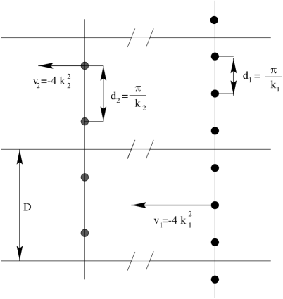
(a)		(b)

Figure 2.1: (a) The motion of the poles of a one-soliton solution in the complex plane. (b) The asymptotic motion of the poles of a two-soliton solution.

Since two solitons of the KdV equation cannot move with the same speed, a two-soliton solution of the KdV equation asymtotically appears as the sum of two one-soliton solutions which are well-separated: the higher-amplitude soliton, which is faster, is to the right of the smaller-amplitude soliton as $t\rightarrow-\infty$. As $t\rightarrow\infty$, the higher-amplitude soliton is to the left of the smaller-amplitude soliton. Hence as $t\rightarrow-\infty$, the pole configuration of a two-soliton solution with wave numbers $k_{1}$ and $k_{2}$ is as in Fig. 2.1b. In this limit, the two-soliton solution is a sum of two one-soliton solutions. Each results in a vertical line of equispaced poles, with interpolar distance respectively $d_{1}=\pi/k_{1}$ and $d_{2}=\pi/k_{2}$. As long as the solitons are well-separated, these poles move in approximately straight lines, parallel to the real axis, with respective velocities $v_{1}=-4k_{1}^{2}$ and $v_{2}=-4k_{2}^{2}$. Since $|v_{1}|>|v_{2}|$, the solitons interact eventually. This interacting results in non-straight line motion of the poles. After the interaction, the situation is as in Fig. 2.1b, but with the two lines of poles interchanged.

Thickstun [thickstun] considered the case where $k_{1}$ and $k_{2}$ are rationally related, so $k_{1}/k_{2}=p/q$, where $p$ and $q$ are positive integers. In this case, one can define $D=pd_{1}=qd_{2}$. The complex $x$-plane is now divided into an infinite number of equal strips, parallel to the real $x$-axis, each of height $D$. The real $x$-axis is usually taken to be the base of such a strip. It is easy to show [thickstun] that the motion of the poles in one strip is repeated in every strip. Hence, one is left studying the motion of a finite number $N$ ($=p+q$) of poles in the fundamental strip, whose base is the real $x$-axis. Thickstun examined this motion by analyzing the exact expression for a two-soliton solution of the KdV equation.

Any two-soliton solution is expressible as [as]

$$u(x,t)=2\partial_{x}^{2}\ln\tau(x,t).$$ (2.5)

It follows from this formula that the poles of $u(x,t)$ are the zeros of $\tau(x,t)$ if $\tau(x,t)$ is entire in $x$. Then the Weierstraß Factorization Theorem [conway] gives a factorization for $\tau(x,t)$:

$$\tau(x,t)=C\prod_{k=1}^{\infty}\left(1-\frac{x}{x_{k}}\right)e^{x/x_{k}}.$$ (2.6)

Since only the second logarithmic derivative of this function is relevant, the constant $C$ is not important. If the solution is periodic in the imaginary $x$-direction, this is rewritten as

$$\tau(x,t)=C\prod_{n=1}^{N}\prod_{l=-\infty}^{\infty}\left(1-\frac{x}{x_{n}+ilD}\right)e^{x/(x_{n}+ilD)},$$ (2.7)

where the first product runs over the poles in the fundamental strip. The second product runs over all strips. Using the uniform convergence of (2.7),

$$u(x,t)=-2\sum_{n=1}^{N}\sum_{l=-\infty}^{\infty}\frac{1}{(x-x_{n}-ilD)^{2}},$$ (2.8)

which, using (2.2), is rewritten as

$$u(x,t)=-2\frac{\pi^{2}}{D^{2}}\sum_{n=1}^{N}\mbox{cosech}^{2}\frac{\pi(x-x_{n})}{D}=-2\frac{k_{2}^{2}}{q^{2}}\sum_{n=1}^{p+q}\mbox{cosech}^{2}\frac{k_{2}(x-x_{n})}{q},$$ (2.9)

where the pole locations $x_{n}$ depend on time: $x_{n}=x_{n}(t)$. One recovers the one-soliton solution (2.1) easily, by equating $k_{1}=0,p=0,q=1$. Equation (2.9) essentially expresses a two-soliton solution as a linear superposition of $N$ one-soliton solutions with nonlinearly interacting phases. Note that the first equality in (2.9) is valid for arbitrary soliton solutions that are periodic in $x$ with period $iD$. This is the case for a g-soliton solution if its wavenumbers $k_{i}$, $i=1,2,\ldots,g$ are all commensurable: $(k_{1}:k_{2}:\ldots:k_{g})=(p_{1}:p_{2}:\ldots:p_{g})$, for positive distinct integers $p_{i}$, $i=1,2,\ldots,g$ which have no overall common integer factor. The total number of poles in a strip is then $N=p_{1}+p_{2}+\ldots+p_{g}$. In obtaining (2.8) and (2.9), we have deviated from Thickstun’s approach [thickstun] to an approach that is generalized to the elliptic case of the next section in a straightforward way.

Next, we derive the dynamics imposed on the poles $x_{n}(t)$ by the KdV equation. This is conveniently done by substituting (2.8) into (1.1) and examining the behaviour near one of the poles: $x=x_{n}+\epsilon$. This results in several singular terms as $\epsilon\rightarrow 0$, corresponding to negative powers of $\epsilon$. The dynamics of the poles is then determined by the vanishing of the coefficients of these negative powers and the zeroth power. This results in only two nontrivial equations, obtained at order $\epsilon^{-3}$ and $\epsilon^{-2}$ respectively:

$$\dot{x}_{n} = 12{\sum_{k=1,k\neq n}^{N}}\sum_{l=-\infty}^{\infty}\frac{1}{(x_{k}-x_{n}-ilD)^{2}}+12\sum_{l\neq 0,l=-\infty}^{\infty}\frac{1}{(-ilD)^{2}},$$ (2.10 a)

$$0 = \sum_{k=1,k\neq n}^{N}\sum_{l=-\infty}^{\infty}\frac{1}{(x_{k}-x_{n}-ilD)^{3}},$$ (2.10 b)

for $n=1,2,\ldots,N$. Using (2.2) and its derivative,

$$\dot{x}_{n} = -4\frac{\pi^{2}}{D^{2}}+12\frac{\pi^{2}}{D^{2}}{\sum_{k=1,k\neq n}^{N}}\mbox{cosech}^{2}\frac{\pi(x_{k}-x_{n})}{D},$$ (2.11 a)

$$0 = \sum_{k=1,k\neq n}^{N}\mbox{cosech}^{2}\frac{\pi(x_{k}-x_{n})}{D}\,\mbox{coth}\frac{\pi(x_{k}-x_{n})}{D},$$ (2.11 b)

for $n=1,2,\ldots,N$. Hence the dynamics of the poles $x_{n}(t)$ is determined by (2.11 a). This dynamics is constrained by the equations (2.11 b). These constraint equations (2.11 b) are invariant under the flow of (2.11 a). This follows from a direct calculation.

Remarks:

• Since the KdV equation has two-soliton solutions for any ratio of the wavenumbers $k_{1}/k_{2}\neq 1$, the constraint (2.11 b) is solvable for any value of $N$, excluding $N=2$, which can only be obtained by $p=q=1$, resulting in equal wavenumbers $k_{1}$ and $k_{2}$.

• In particular, it follows that the minimum number of poles in a fundamental strip required to obtain a $g-soliton$ solution is $N=1+2+3+\ldots+g=g(g+1)/2$, corresponding to a $g$-soliton solution with wavenumbers which are related as $(k_{1}:k_{2}:\ldots:k_{g-1}:k_{g})=(g:g-1:\ldots:2:1)$.

• Equating $k_{1}=0$, $p=0$, $q=1$, one obtains from (2.11 a) $\dot{x}_{1}=-4k_{2}^{2}$, corresponding to the dynamics of the one-soliton solution. The asymptotic behavior of the poles of a two-soliton solution also follows from (2.11 a): from the separation of the poles into distinct vertical lines, it follows from (1.4 a) that the velocity of these vertical lines is given by the one-soliton velocity for each line, as expected. This result follows from easy algebraic manipulation and the identity

  $$\frac{p^{2}-1}{3}=\sum_{n=1}^{p-1}\mbox{cosec}^{2}\left(\frac{n\pi}{p}\right),$$

  valid for any integer $p>1$.

• A full analysis of the interaction of the poles for the case of any two-soliton solution with $k_{1}/k_{2}=p/q$ is given in [thickstun].

3 The elliptic case

Consider the quasiperiodic finite-gap solutions of the KdV equation with $g$ phases [itsmatveev]

$$u(x,t)=2\partial_{x}^{2}\ln\theta_{g}(\mbox{\boldmath{$k$}}x+\mbox{\boldmath{$\omega$}}t+\mbox{\boldmath{$\phi$}}|\mbox{\boldmath{$B$}}),$$ (3.1)

where

$$\theta_{g}(\mbox{\boldmath{$z$}}|\mbox{\boldmath{$B$}})=\sum_{\mbox{\boldmath{$m$}}\in\mbox{\boldmath{$Z^{g}$}}}\exp\left(\frac{1}{2}\mbox{\boldmath{$m$}}\cdot\mbox{\boldmath{$B$}}\cdot\mbox{\boldmath{$m$}}+i\mbox{\boldmath{$m$}}\cdot\mbox{\boldmath{$z$}}\right),$$ (3.2)

a hyperelliptic Riemann-theta function of genus $g$. The $g\times g$ real Riemann matrix ($i.e.$, symmetric and negative definite) $B$ originates from a hyperelliptic Riemann surface with only one point at infinity. Furthermore, $k$, $\omega$ and $\phi$ are $g$-dimensional vectors.

The derivation of equations (2.9), (2.11 a) and (2.11 b) is easily generalized to the case where the solution is not only periodic in the imaginary $x$-direction, but also in the real $x$-direction:

$$u(x+L_{1},t)=u(x,t)=u(x+iL_{2},t).$$ (3.3)

This divides the complex $x$-plane into an array of rectangular domains, each of size $L_{1}\times L_{2}$. One of these domains, called the fundamental domain $S$, is conveniently placed in the lower left corner of the first quadrant of the $x$-plane. The theta function has the property [dub]

$$\theta_{g}(\mbox{\boldmath{$z$}}+i\mbox{\boldmath{$B$}}\cdot\mbox{\boldmath{$M$}}+2\pi\mbox{\boldmath{$N$}}|\mbox{\boldmath{$B$}})=\theta_{g}(\mbox{\boldmath{$z$}}|\mbox{\boldmath{$B$}})\exp\left(-\frac{1}{2}\mbox{\boldmath{$M$}}\cdot\mbox{\boldmath{$B$}}\cdot\mbox{\boldmath{$M$}}+i\mbox{\boldmath{$M$}}\cdot\mbox{\boldmath{$z$}}\right),$$ (3.4)

for any pair of $g$-component integer vectors $\mbox{\boldmath{$M$}},\mbox{\boldmath{$N$}}$. This expression is useful to determine conditions on the wavevector $k$ in order for $u(x,t)$, given by (3.1), to satisfy (3.3):

$$\exists~{}\mbox{\boldmath{$N_{0}$}},\mbox{\boldmath{$M_{0}$}}\in\mbox{\boldmath{$Z$}}^{g}:\mbox{\boldmath{$k$}}L_{1}=2\pi\mbox{\boldmath{$N_{0}$}},~{}\mbox{\boldmath{$k$}}L_{2}=\mbox{\boldmath{$B$}}\cdot\mbox{\boldmath{$M_{0}$}}.$$ (3.5)

These results are now used to determine the number of poles $N$ of $u(x,t)$ in the fundamental domain. The poles of (3.1) are given by the zeros of $\vartheta(x,t)=\theta_{g}(\mbox{\boldmath{$k$}}x+\mbox{\boldmath{$\omega$}}t+\mbox{\boldmath{$\phi$}}|\mbox{\boldmath{$B$}})$, regarded as a function of $x$:

$$N = \frac{1}{2\pi i}\oint_{\partial S}d\ln\vartheta(x,t)$$ (3.6)

$$= \frac{1}{2\pi i}\left(\int_{0}^{L_{1}}d\ln\vartheta(x,t)+\int_{0}^{iL_{2}}d\ln\vartheta(x+L_{1},t)-\right.$$

$$\left.\int_{0}^{L_{1}}d\ln\vartheta(x+iL_{2},t)-\int_{0}^{iL_{2}}d\ln\vartheta(x,t)\right)$$

$$\stackrel{{\scriptstyle\mbox{using (\ref{thetaprop})}}}{{=}} \frac{1}{2\pi i}\int_{0}^{L_{1}}d\ln\frac{\vartheta(x,t)}{\vartheta(x+iL_{2},t)}$$

$$\stackrel{{\scriptstyle\mbox{using (\ref{thetaprop})}}}{{=}} \frac{1}{2\pi i}\int_{0}^{L_{1}}d(-ix\mbox{\boldmath{$M_{0}$}}\cdot\mbox{\boldmath{$k$}})$$

$$= -\mbox{\boldmath{$M_{0}$}}\cdot\mbox{\boldmath{$N_{0}$}}=-\frac{L_{1}}{2\pi L_{2}}\mbox{\boldmath{$M_{0}$}}\cdot\mbox{\boldmath{$B$}}\cdot\mbox{\boldmath{$M_{0}$}}.$$

The first equality of (3.6) confirms that $N$ is an integer. The second equality shows that $N$ is positive, by the negative-definiteness of $B$.

We now proceed to determine the dynamical system satisfied by the motion of the $N$ poles of $u(x,t)$ in the fundamental domain $S$. Again, the poles of $u(x,t)$ are the zeros of $\vartheta(x,t)$. Furthermore, simple zeros of $\vartheta(x,t)$ result in double poles of $u(x,t)$, as in the hyperbolic case.

The Weierstraß Factorization theorem [conway] gives the following form for $\vartheta(x,t)$:

$$\vartheta(x,t)=e^{cx^{2}/2}\prod_{k}\left(1-\frac{x}{x_{k}}\right)e^{\frac{x}{x_{k}}+\frac{x^{2}}{2x_{k}^{2}}},$$ (3.7)

where the product runs over all poles $x_{k}$. The additional exponential factors, as compared to (2.6), are required because the poles now appear in a bi-infinite sequence: both in the vertical and horizontal directions. These exponential factors ensure uniform convergence of the product. The parameter $c$ is allowed to depend on time. It determines the behavior of $\vartheta(x,t)$ as $x$ approaches infinity in the complex $x$-plane [dub]. Using (3.3), this is rewritten as

$$\vartheta(x,t)=\exp(cx^{2}/2)\prod_{n=1}^{N}\prod_{m=-\infty}^{\infty}\prod_{l=-\infty}^{\infty} \!\!\!\!\!\!\!\!\!\!\left(1-\frac{x}{x_{n}+mL_{1}+ilL_{2}}\right)\times$$ (3.8)

$$\!\!\!\!\!\!\!\!\!\!\exp\left(\frac{x}{x_{n}+mL_{1}+ilL_{2}}+\frac{x^{2}}{2(x_{n}+mL_{1}+ilL_{2})^{2}}\right).$$

The first product runs over the number of poles ($N$) in the fundamental domain, the second and third products result in all translations of the fundamental domain. From the uniform convergence of (3.8),

$$u(x,t)=2c-2\sum_{n=1}^{N}\sum_{m=-\infty}^{\infty}\sum_{l=-\infty}^{\infty}\left(\frac{1}{(x-x_{n}-mL_{1}-ilL_{2})^{2}}-\frac{1}{(x_{n}+mL_{1}+ilL_{2})^{2}}\right).$$ (3.9)

Using the definition of the Weierstraß function (1.3), this is rewritten as

$$u(x,t)=2c-2\sum_{n=1}^{N}\wp(x-x_{n})+2\sum_{j=1}^{N}\wp(x_{n}),$$ (3.10)

where the periods of the Weierstraß function are given by $2\omega_{1}=L_{1},2\omega_{2}=iL_{2}$. Define

$$\tilde{c}=2c+2\sum_{n=1}^{N}\wp(x_{n}).$$ (3.11)

The dynamics of the poles $x_{n}=x_{n}(t)$ is determined by substitution of (3.10) or (3.9) into the KdV equation and expanding in powers of $\epsilon$ for $x$ near a pole: $x=x_{k}+\epsilon$. Equating the coefficients of $\epsilon^{-3}$, $\epsilon^{-2}$ and $\epsilon^{0}$ to zero result in

$$\dot{x}_{n} = 12\sum_{j=1,j\neq n}^{N}\wp(x_{j}-x_{n}),$$ (3.12 a)

$$0 = \sum_{j=1,j\neq n}^{N}\wp^{\prime}(x_{j}-x_{n}),$$ (3.12 b)

$$\dot{\tilde{c}} = 0\Leftrightarrow\tilde{c}(t)=\alpha=0,$$ (3.12 c)

for $n=1,2,\ldots,N$. (The constant $\alpha$ can always be removed by a Galilean shift, so it is equated to zero, without loss of generality.) The constraints (3.12 b) are invariant under the flow, as can be checked by direct calculation. Notice that (3.12 a-b) are identical to the equations obtained by Airault, McKean and Moser [amm]. These equations are obtained here in greater generality: any solution (3.1) which is doubly periodic in the $x$-plane gives rise to a system (3.12 a-b). This allows us to reach the conclusions stated in the next section.

Remarks

• In the limit $L_{1}\rightarrow\infty$, the equations (3.12 a–3.12 b) reduce to (2.11 a–2.11 b). This limit is most conveniently obtained from the Poisson representation of the Weierstraß function:

  $$\wp(x)=\left(\frac{\pi}{L_{2}}\right)^{2}\left(\frac{1}{3}+\mbox{cosech}^{2}\frac{\pi x}{L_{2}}+\sum_{n=-\infty,n\neq 0}^{\infty}\left\{\mbox{cosech}^{2}\frac{\pi}{L_{2}}(x+nL_{1})-\mbox{cosech}^{2}\frac{n\pi L_{1}}{L_{2}}\right\}\right).$$ (3.13)

  This representation is obtained from (1.3) by working out the summation in the vertical direction. It gives the Weierstraß function as a sum of exponentially localized terms, hence few terms have important contributions in the fundamental domain. A Poisson expansion for $\wp^{\prime}(x)$ is obtained from differentiating (3.13) term by term with respect to $x$.

• Define the one-phase theta function $\theta_{1}(z,q)$ [tables]:

  $$\theta_{1}(z,q)=2\sum_{n=0}^{\infty}(-1)^{n}q^{(n+1/2)^{2}}\sin(2n+1)z,$$ (3.14)

  with $|q|<1$. If $L_{2}<L_{1}$, then the relationship $\wp(z)=a-\partial_{x}^{2}\ln\theta_{1}(\pi z/L_{1},iL_{2}/L_{1})$, with $a$ a constant [tables], allows us to rewrite (1.2) as

  $$u(x,t)=\hat{a}+2\partial_{x}^{2}\ln\prod_{j=1}^{N}\theta_{1}\left(\frac{\pi}{L_{1}}(x-x_{j}(t)),i\frac{L_{2}}{L_{1}}\right),$$ (3.15)

  with $\hat{a}=-2aN$. Hence, for the doubly-periodic solutions of the KdV equation of the form (3.1), it is possible to rewrite the $g$-phase theta function as a product of $N$ $1$-phase theta functions, with nonlinearly interacting phases. Note that this does not imply that the $g$-phase theta function appearing in (3.1) is reducible. Reducible theta-functions do not give rise to solutions of the KdV equation [dub].

• By taking another time derivative of (3.12 a) and using (3.12 b), one obtains

  $$\ddot{x}_{n}=-(12)^{2}\sum_{j=1,j\neq n}^{N}\wp^{\prime}(x_{j}-x_{n})\wp(x_{j}-x_{n}).$$ (3.16)

  It is known that this system of differential equations is Hamiltonian [chud], with Hamiltonian

  $$H=\frac{1}{2}\sum_{k=1}^{N}p_{k}^{2}+\frac{(12)^{2}}{2}\sum_{k=1}^{N}\sum_{j=1,j\neq k}^{N}\wp^{2}(x_{k}-x_{j}),$$ (3.17)

  and canonical variables $\{x_{k},p_{k}=\dot{x}_{k}\}$. A second Hamiltonian structure for the equations (3.16) is given in [chud]. A Lax representation for the system (3.12 a-c) is also given there. This Lax representation is a direct consequence of the law of addition of the Weierstraß function [tables]. It is unknown to us whether a Hamiltonian structure exists for the constrained first-order dynamical system (3.12 a-b).

  The Hamiltonian structure (3.17) shows that the system (3.12 a-b) is a (constrained) member of the elliptic Calogero-Moser hierarchy [belokolos1].

4 Discussion of the dynamics

In this section, the constrained dynamical system (3.12 a-c) is discussed. In particular, the assertions made in the introduction are validated here.

For reality of the KdV solution (3.1) when $x$ is restricted to the real line, it is necessary and sufficient that if $x_{j}(t)$ appears, then so does $x_{j}^{*}(t)$. Because the Weierstraß function is a meromorphic functions of its argument, this reality constraint is invariant under the dynamics (3.12 a).

As a consequence, the distribution of the poles in the fundamental domain $S$ is symmetric with respect to the horizontal centerline of $S$. Poles are allowed on the centerline. Most of what follows is valid for both real KdV solutions and KdV solutions that are not real, but we restrict our attention to real KdV solutions.

4.1 All finite-gap elliptic solutions of the KdV equation are of the form (1.2), up to a constant

A straightforward singularity analysis of the KdV equation [amm] shows that any algebraic singularity of a solution of the KdV equation is of the type $u(x,t)=-2/(x-\alpha(t))^{2}+{\cal O}(x-\alpha)$, for almost all times t. At isolated times $t_{c}$, the leading order coefficient is not necessarily $-2$. It can be of the form $-g(g+1)$ (see below), but the exponent of the leading term is always $-2$.

Hence, an elliptic function ansatz for $u(x,t)$ can only have second order poles and with the substitution $u(x,t)=2\partial_{x}^{2}\ln\vartheta(x,t)$ gives rise to a Weierstraß expansion of the form (3.8), with an arbitrary prefactor $\exp(c(x,t))$, for an arbitrary function $c(x,t)$, entire in $x$. Substitution of this ansatz in the KdV equation then determines that $c_{xx}$ is doubly periodic and meromorphic in $x$. The only such $c$ is a constant. Hence, all finite-gap elliptic solutions of the KdV equation are of the form (1.2).

4.2 If $L_{1}/L_{2}\gg 1$, any number of poles $N\neq 2$ in the fundamental domain is allowed

We have already argued that the equations (2.9) and (2.11 a-b) are obtained from (1.2) and (3.12 a-b) in the limit $L_{1}\rightarrow\infty$. On the other hand, (3.13) can be regarded as a perturbative expansion of the soliton case, which corresponds to its first two terms. Because (3.13) converges uniformly away from $x=n_{1}L_{1}+in_{2}L_{2}$, for arbitrary integers $n_{1},n_{2}$ we conclude that for large (but finite) values of $L_{1}/L_{2}$ any real, nonsingular $g$-soliton solution with rationally related wave numbers $(k_{1}:k_{2}:\ldots:k_{g})=(p_{1}:p_{2}:\ldots:p_{g})$ has an elliptic deformation with real period $L_{1}$ and imaginary period $iL_{2}$, which is real and nonsingular. Since $N=p_{1}+p_{2}+\dots+p_{g}\neq 2$ is arbitrary in the soliton case, this is also true for these elliptic deformations of the solitons. Hence the constraint (3.12 b) is solvable for arbitrary $N$, for $L_{1}\gg L_{2}$.

At this point, it is appropriate to remark that if one is interested in elliptic solutions of the Kadomtsev-Petviashvili (KP) equation,

$$\partial_{x}\left(-u_{t}+6uu_{x}+u_{xxx}\right)+3\sigma^{2}u_{yy}=0$$ (4.1)

(with parameter $\sigma$), then the equations (1.2), (3.12 a-b) are replaced by [chud]

$$u(x,y,t) = -2\sum_{n=1}^{N}\wp(x-x_{n}(y,t)),$$ (4.2 a)

$${\partial x_{n}\over\partial t} = 3\sigma^{2}\left({\partial x_{n}\over\partial y}\right)^{2}+12\sum_{j=1,j\neq n}^{N}\wp(x_{j}-x_{n}),$$ (4.2 b)

$$\sigma^{2}{\partial^{2}x_{n}\over\partial y^{2}} = -16\sum_{j=1,j\neq n}^{N}\wp^{\prime}(x_{j}-x_{n}).$$ (4.2 c)

This clarifies the appearance of the constraint (3.12 b) on the motion of the poles of elliptic solutions of the KdV equation, where the poles are independent of $y$. The search for $y$-independent solutions of the KP equation reduces it to the KdV equation and it reduces the equations (4.2 a-c) to (1.2), (3.12 a-b), forcing the poles to remain on the invariant manifold defined by (3.12 b). For the KP equation, no such constraint exists and hence the number of poles $N$ in the fundamental domain can be any integer, not equal to two.

4.3 For any $N>4$, nonequivalent configurations exist, for $L_{1}/L_{2}$ sufficiently large

Again, we only consider solutions with nonsingular soliton limits; $i.e.,$ the elliptic deformations mentioned above. Consider the asymptotic behavior for $t\rightarrow-\infty$ of $\lim_{L_{1}\rightarrow\infty}u(x,t)$. In this soliton limit, as $t\rightarrow-\infty$, the poles are collected in groups corresponding to one-soliton solutions.

In this section, two configurations are called nonequivalent if the above asymptotic behavior results in a different grouping of the poles.

For $N=3$, all configurations are equivalent to one configuration. In the limit $L_{1}\rightarrow\infty$, this configuration corresponds to the two-soliton case with $k_{1}:k_{2}=2:1$. This configuration is discussed in Section 5.1.

For $N=4$, all configurations are again equivalent to one configuration. This configuration corresponds to the two-soliton case with $k_{1}:k_{2}=3:1$. Recall that $k_{1}$ and $k_{2}$ are not allowed to be equal, hence a configuration with two poles to the left and two poles to the right does not exist. Another way of expressing that only one configuration exists is that $N=4$ can only be decomposed as the sum of distinct positive integers without common factor as $N=3+1$. Again, all $N=4$ configurations are equivalent. This configuration is discussed in Section 5.2. That section also discusses another example of an $N=4$ potential which does not have a nonsingular soliton limit. This potential is a special case of one of the Treibich-Verdier potentials (1.8).

Any integer $N>4$ can be written as a sum of distinct positive integers without overall common factor in more than one way. Let the number of terms in the $m$-th decomposition of $N$ be denoted as $N_{m}$, then $N=\sum_{i=1}^{N_{m}}n_{i}$, with the $n_{i}$ distinct and having no overall common factor. This configuration corresponds to the $N_{m}$-soliton case with wavenumber ratios $(k_{1}:k_{2}:\ldots:k_{N_{m}})=(n_{1}:n_{2}:\ldots:n_{N_{m}})$. A solution with these wave numbers has $N_{m}$ phases and is an $N_{m}$-soliton solution. Hence for any $N>4$ there exist at least as many different configurations as there are decompositions of $N$ into distinct positive integers, without overall common factor. These configurations need not have the same number of phases.

Two nonequivalent configurations corresponding to $N=5$ are discussed in Section 5.3.

4.4 The poles only collide in triangular numbers

A collision of poles is a local process in which only the colliding poles play a significant role. The analysis of the collisions is identical to the rational and the soliton cases because close to the collision point, the Weierstraß function reduces to $1/x^{2}$. Kruskal [kruskalpoles] already noticed that the poles do not collide in pairs, but triple collisions do occur. In fact, any triangular number of poles can participate in a collision, in which case the solution of the KdV equation at the collision time $t_{c}$, nearby the collision point $x_{c}$ is given by $u(x,t_{c})=-g(g+1)/(x-x_{c})^{2}$ [amm]. Asymtotically near the collision point $x_{c}$, $i.e.,$ $t<t_{c}$, the poles lie on the vertices of a regular polygon with $g(g+1)/2$ vertices. For $t>t_{c}$, the poles emanate from the collision points, again forming a regular polygon with $g(g+1)/2$ vertices. If $g(g+1)/2$ is even, this polygon is identical to the polygon before the collision. If $g(g+1)/2$ is odd, the polygon is rotated around the collision point by $2\pi/g(g+1)$ radians.

Of all these collision types, the one where three poles collide (corresponding to $g=1$) is generic. It is the one observed in the examples illustrated in Section 5.

Since the poles only collide in triangular numbers, it is possible that at any given time $t_{c}$ the solution of the KdV equation has the form (1.9), with not all $g_{i}=1$. At almost every other time $t$, such a solution has $N=\sum_{i=1}^{M}g_{i}(g_{i}+1)/2$ distinct poles.

4.5 The solutions (1.2) are finite-gap potentials of the stationary Schrödinger equation (1.6)

By construction the solutions (1.2) are periodic in $x$ because they are obtained as a Weierstraß factorization of the theta function appearing in (3.1), upon which we have imposed the double periodicity. Hence the solutions (1.2) are finite-gap potentials of the Schrödinger operator. In [gw2], another proof of this can be found.

For solutions that are elliptic deformations of the nonsingular solitons of Section 2, more can be said: an elliptic deformation of a $g$-soliton solution is a $g$-gap potential of the Schrödinger equation. The reasoning is as follows: we already know that any elliptic deformation results in a finite-gap potential of the Schrödinger equation. On the other hand, any finite gap potential of the Schrödinger equation is of the form (3.1). The soliton limit of such a finite-gap solution with $g$-phases is a $g$-soliton solution [belokolos1]. Hence the number of phases of an elliptic deformation of a $g$-soliton solution is equal to $g$.

This limit is the soliton limit of the periodic solutions, in which the fundamental domain reduces to the fundamental strip. In order to have a $g$-soliton solution of the KdV equation, we remarked in Section 2 that at least $N=g(g+1)/2=1+2+\ldots+g$ poles are required in the fundamental strip. Hence, this many poles are required in the fundamental domain to obtain a $g$-gap potential of the Schrödinger equation that is an elliptic deformation of a nonsingular soliton solution.

5 Examples

In this section, some explicit examples of elliptic solutions of the KdV equation are discussed. These are illustrated with figures displaying the motion of the poles in the fundamental domain. Other figures display the solution of the KdV equation $u(x,t)$ as a function of $x$ and $t$. All these figures were obtained from numerical solutions of the corresponding constrained dynamical system. In all cases, the constrained dynamical system was solved using a projection method: the dynamical system (3.12 a) is used to evolve the system for some time. Subsequently, the new solution is projected onto the constraints (3.12 b) to correct numerical errors, after which the process repeats.

In all examples given, $L_{1}=4$ and $L_{2}=\pi$. This seems to indicate that one can wander far away from $L_{1}/L_{2}\gg 1$ and still obtain soliton-like elliptic solutions of the KdV equation. This is not surprising as (3.13) indicates that as perturbation parameter on the soliton case one should use $\epsilon=\exp(-2\pi L_{1}/L_{2})$. For the values given above, this gives $\epsilon=0.00034$.

5.1 The solution of Dubrovin and Novikov [dubnov]: $N=3$

Dubrovin and Novikov [dubnov] integrated the KdV equation with the Lamé-Ince potential $u(x,0)=-6\wp(x-x_{c})$ as initial condition. They found the solution to be elliptic for all time, with $N=3$. They gave explicit formulae for the solution, which they remarked was probably the simplest two-gap solution of the KdV equation. The dynamics of the poles in the fundamental domain is displayed in Fig. 5.1a. Fig. 5.1b displays the corresponding two-phase solution of the KdV equation. Animations of the behavior of the poles and of $u(x,t)$ as $t$ changes are also available at http://amath-www.colorado.edu/appm/other/kp/papers. Notice the soliton-like interactions of the two phases in the solution. In terms of the classification of Lax [lax2], these are interactions of type (c) ($i.e.,$ $u(x,t)$ has only one maximum while the larger wave overtakes the smaller wave).

From Fig. 5.1a, it appears that the Dubrovin-Novikov solution is periodic in time. This was indeed proven by Ènol’skii [enolskii].

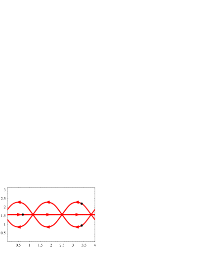
(a)	(b)

Figure 5.1: The solution of Dubrovin and Novikov, with $L_{1}=4$ and $L_{2}=\pi$. (a) The motion of the poles in the fundamental domain. The initial position of the poles is indicated by the black dots. The arrows denote the motion of the poles. (b) The KdV solution $u(x,t)$

For this specific solution only one of the three constraint equations is independent: since the derivative of the Weierstraß function is odd, the sum of the constraints is zero. Furthermore, labelling the three poles by $x_{1},x_{2}$ and $x_{3}$, for reality $x_{2}=x_{1}^{*}+iL_{2}$ and $x_{3}$ is on the centerline. Hence the second constraint is the complex conjugate of the first constraint. The constraints (3.12 b) reduce to the single equation

$$\wp^{\prime}(x_{1}-x_{1}^{*})+\wp^{\prime}(x_{1}-x_{3})=0.$$ (5.1)

This equation was solved numerically to provide the initial condition shown in Fig. 5.1a. The initial guess required for the application of Newton’s method is based on the knowledge of the soliton limit. In that case two poles on the right represent a faster soliton, one pole on the left represents the slower soliton. The periodic case is not that different: the vertical line of poles with the smallest vertical distance between poles has poles closer to the real $x$-axis than the others and correspond to the wave crest with the highest amplitude, as seen in Fig. 5.1b. We refer to the Dubrovin-Novikov solution as a $(2:1)$-solution because of the natural separation of the poles in a group of 2 poles $(x_{1},x_{2})$ and a single pole $(x_{3})$.

Equating $x_{1}=x_{3}+\epsilon$ and only condering the singular terms of (5.1), it is possible to examine the location of the poles close to a collision points $x_{c}$. With $\wp^{\prime}(x)=-2/x^{3}$ in this limit and $\epsilon=\epsilon_{r}+i\epsilon_{i}$, one finds

$$\epsilon_{r}^{3}-3\epsilon_{i}^{2}\epsilon_{r}=0,~{}~{}~{}~{}9\epsilon_{i}^{3}-3\epsilon_{r}^{2}\epsilon_{i}=0.$$ (5.2)

This set of equations has three solutions, corresponding to the three distances between the poles: $\epsilon_{r}/\epsilon_{i}\in\left\{0,\sqrt{3},-\sqrt{3}\right\}$. This allows for two triangular configurations of the poles: an equilateral triangle pointing left of the collision point and one pointing right.

Using the dynamical system (3.12 a) in the same way and only retaining singular terms results in

$$\dot{\epsilon}_{r}=-\frac{3}{4\epsilon_{i}^{2}}+3\frac{\epsilon_{r}^{2}-\epsilon_{i}^{2}}{\left(\epsilon_{r}^{2}+\epsilon_{i}^{2}\right)^{2}},~{}~{}~{}~{}\dot{\epsilon}_{i}=\frac{6\epsilon_{r}\epsilon_{i}}{\left(\epsilon_{r}^{2}+\epsilon_{i}^{2}\right)^{2}}.$$ (5.3)

Since the constraints (3.12 b) are invariant under the flow (3.12 a), the solutions to (5.2) give invariant directions of the system (5.3). Along these invariant directions, one obtains ordinary differential equations for the motion of the poles as they approach the collision point. It follows from these equations that the poles approach the collision point $x_{c}$ with infinite velocity. Integrating the equations with initial condition $\epsilon(t_{c})=0$ gives

$$\epsilon=\frac{3^{5/6}}{2}(\sqrt{3}+i)(t_{c}-t)^{1/3}.$$ (5.4)

Using the three branches of $(t_{c}-t)^{1/3}$ results in the dynamics of each edge of the equilateral triangle. If $t<t_{c}$ this triangle is pointing left, for $t>t_{c}$ it is pointing right.

5.2 $N=4$: an elliptic deformation and a Treibich-Verdier solution

The next solution we discuss has 4 poles in the fundamental domain and is an elliptic deformation of a soliton solution. In the limit $L_{1}\rightarrow\infty$, this solution corresponds to a two-soliton solution with wavenumber ratio $k_{1}/k_{2}=3/1$, so this solution is refered to as a $(3:1)$- solution.

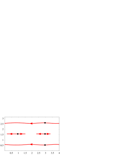
Figure 5.2: $N=4$: the pole dynamics of a $(3:1)$-solution. The initial positions of the 4 poles are indicated. The arrows on the centerline indicate that the poles there move in both directions.

The motion of the poles in the fundamental domain is displayed in Fig. 5.2. Corresponding to the given wavenumber ratio, the amplitute ratio of the two phases present in the solution is roughly $k_{1}^{2}/k_{2}^{2}=9/1$. As a consequence, the form of $u(x,t)$ is not very illuminating and it has been omitted. Animations with the time dependence of both the positions of the poles and of $u(x,t)$ are again available at http://amath-www.colorado.edu/appm/other/kp/papers.

Note that the poles of the $(3:1)$-solution do not collide. This is in agreement with the results of Thickstun [thickstun] who outlined which configurations lead to collisions and which do not, in the hyperbolic case. As mentioned before, the examination of collision behavior is essentially local and no differences appear between the rational, hyperbolic and elliptic cases.

Another configuration with $N=4$ exists. Consider the potential

$$u(x,t=t_{c})=-2\wp(x-x_{0})-6\wp(x-x_{0}-\omega_{1}),$$ (5.5)

with $x_{0}$ on the centerline. This is a Treibich-Verdier potential, obtained from (1.9) with $M=2$, $g_{1}=1$, $g_{2}=2$, $\alpha_{1}=x_{0}$ and $\alpha_{2}=x_{0}+\omega_{1}$. It is referred to as a Treibich-Verdier potential because the position of the poles is given in terms of the periods of the Weierstraß function, as in (1.8). Also, it can be obtained from (1.8) as a degenerate case. As before $N=\sum_{i=1}^{2}g_{i}(g_{i}+1)/2=4$, hence for all times that are not collision times, this solution has 4 distinct poles in the fundamental domain. The time $t=t_{c}$ is a collision time. Immediately after the collision time $t=t_{c}$, the 3 poles located at $x_{0}+\omega_{1}$ separate, as in the Dubrovin-Novikov solution, along an equilateral triangle. The result appears to be a three-phase solution. However, it is known that the potential (5.5) is a two-gap potential of the Schrödinger equation and its hyperelliptic Riemann surface is given explicitly in [belokolos1]. This solution is not an elliptic deformation of a nonsingular soliton solution and the separation into different phases does not make sense. This is also seen from the following argument: if, for a fixed time which is not a collision time, we attempt to take the limit as $L_{1}=2\omega_{1}\rightarrow\infty$, the poles seem to separate in three distinct solitons with respective wave numbers $(k_{1}:k_{2}:k_{3})=(2:1:1)$. Such a nonsingular soliton solution does not exist for the KdV equation and the separation into different phases does not make sense.

The dynamics of the poles is illustrated in Fig. 5.3a. The corresponding KdV solution is shown in Fig. 5.3b.

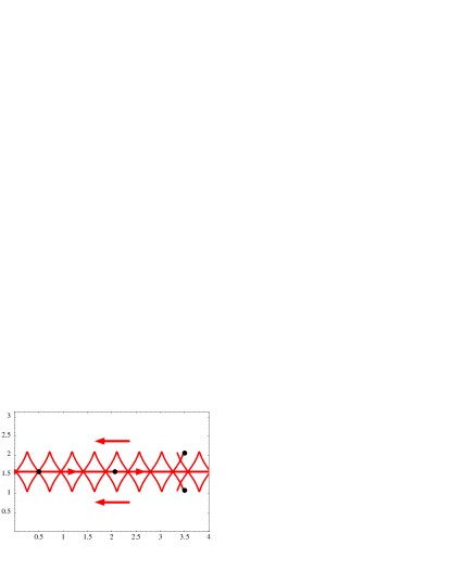
(a)	(b)

Figure 5.3: An $N=4$, $M=2$ Treibich-Verdier solution, with $L_{1}=4$ and $L_{2}=\pi$. (a) The motion of the poles in the fundamental domain. The initial position of the poles is indicated by the black dots. The initial time $t=0$ was chosen different from the collision times $t_{c}$. The arrows denote the motion of the poles. (b) The KdV solution $u(x,t)$

The dynamics of the poles illustrated in Fig. 5.3a exhibits behavior that appears qualitatively different from any other solution discussed here. The trajectories traced out by the motion of the poles in the fundamental domain appear to have singular points (cusps), away from the collision points. Upon closer investigation, these “cusps” are only a figment of the resolution of the plot and the poles trace out a regular curve as a function of time, away from the collision times. Exactly why the global pole dynamics of the Treibich-Verdier potential (5.5) under the KdV flow appears so different from the pole dynamics of elliptic deformations of soliton solutions of the KdV equation is an open problem. Another question one may ask is whether similar behavior is observed for other solutions originating from Treibich-Verdier potentials.

5.3 $N=5$: two different possibilities

For $N=5$, two soliton configurations are possible, and corresponding to each of these is an elliptic solution. The first solution is a $(4:1)$-solution. The second solution is a $(3:2)$-solution.

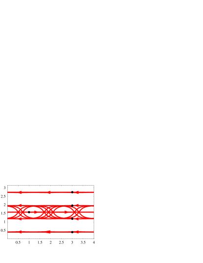
(a)
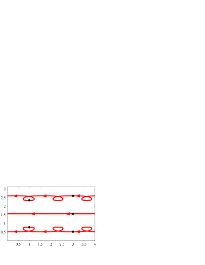
(b)	(c)

Figure 5.4: $N=5$: (a) The pole dynamics of a $(4:1)$-solution in the fundamental domain. (b) The pole dynamics of a $(3:2)$-solution in the fundamental domain. (c) The KdV solution $u(x,t)$ corresponding to the pole dynamics in (b). In (a) and (b), the initial positions of the poles are indicated. Both solutions are quasiperiodic in time. $u(x,t)$

The $(4:1)$-solution offers no new pole-dynamics: initially 1 pole is located on the centerline, at the left in the fundamental domain. The other poles are located at the right of the fundamental domain, symmetric with respect to the centerline. The three poles closest to the centerline interact as the $(2:1)$-solution. The two outer poles behave as the two outer poles of the $(3:1)$-solution. The pole dynamics of the $(4:1)$-solution is displayed in Fig. 5.4a.

The $(3:2)$-solution is more interesting. It is displayed in Fig. 5.4c, together with the motion of the poles in the fundamental domain 5.4b. Again, the two crests of $u(x,t)$ interact in a soliton-like manner. In Lax’s classification [lax2], this is an interaction of type (a), where at every time two maxima are observed. Fig. 5.4b only displays the motion of the poles for a short time, in order not to clutter the picture. The motion of the poles is presumably quasiperiodic in time, as is the case for the $(4:1)$-solution. It appears that the two poles above (or below) the middle line of the fundamental domain share a common trajectory. It is an open problem to establish whether or not this is the case.

5.4 $N=6$: two different possibilities. A three-phase solution

For $N=6$, two distinct pole configurations are possible. The first one corresponds to a $(5:1)$-solution and results in a two-gap potential of the Schrödinger equation. It essentially behaves as the $(3:1)$-solution with two more poles added, which also behave as the outer poles of the $(3:1)$-solution.

The second configuration is a $(3:2:1)$-solution, which limits to a three-soliton solution with wavenumber ratio $(k_{1}:k_{2}:k_{3})=(3:2:1)$. This elliptic solution is a three-phase solution of the KdV equation.

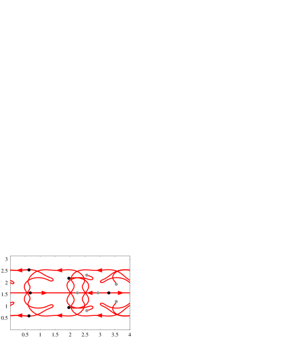
Figure 5.5: The pole dynamics of a $(3:2:1)$-solution. The black dots mark the initial position of the poles; the grey dots mark the position of the poles at $t=0.4$.

Figure 5.6: A $(3:2:1)$-solution of the KdV equation, corresponding to the pole dynamics in Fig. 5.6

The amplitude ratio of the $(3:2:1)$-solution is $(9:4:1)$, which explains why the third phase is hard to notice in Fig. 5.6. Animations of the pole dynamics and of the time dependence of the $(3:2:1)$-solution are available at http://amath-www.colorado.edu/appm/other/kp/papers.