Integrable vs Nonintegrable
Geodesic Soliton Behavior

Abstract

We study confined solutions of certain evolutionary partial differential equations (pde) in $1+1$ space-time. The pde we study are Lie-Poisson Hamiltonian systems for quadratic Hamiltonians defined on the dual of the Lie algebra of vector fields on the real line. These systems are also Euler-Poincaré equations for geodesic motion on the diffeomorphism group in the sense of the Arnold program for ideal fluids, but where the kinetic energy metric is different from the $L^{2}$ norm of the velocity. These pde possess a finite-dimensional invariant manifold of particle-like (measure-valued) solutions we call “pulsons.” We solve the particle dynamics of the two-pulson interaction analytically as a canonical Hamiltonian system for geodesic motion with two degrees of freedom and a conserved momentum. The result of this two-pulson interaction for rear-end collisions is elastic scattering with a phase shift, as occurs with solitons. In contrast, head-on antisymmetric collisons of pulsons tend to form singularities.

Numerical simulations of these pde show that their evolution by geodesic dynamics for confined (or compact) initial conditions in various nonintegrable cases possesses the same type of multi-soliton behavior (elastic collisons, asymptotic sorting by pulse height) as the corresponding integrable cases do. We conjecture this behavior occurs because the integrable two-pulson interactions dominate the dynamics on the invariant pulson manifold, and this dynamics dominates the pde initial value problem for most choices of confined pulses and initial conditions of finite extent.

¹Dept. of Civil and Environmental Engineering, Stanford University, Stanford, CA 94305. email: fringer@leland.stanford.edu, www: http://rossby.stanford.edu/^∼fringer

²Theoretical Division and Center for Nonlinear Studies, Los Alamos National Laboratory, Los Alamos, NM 87545. email: dholm@lanl.gov, www: http://cnls.lanl.gov/^∼dholm

1 Introduction

We study particle-like dynamics on a set of finite-dimensional invariant manifolds for certain measure-valued solutions, called “pulsons,” of the family of evolutionary integral partial differential equations given by

$$m_{t}+um_{x}+2mu_{x}=0\,,\quad\lim_{|x|\to\infty}m=0\,.$$ (1.1)

Here subscripts denote partial derivatives, $m:\mathbb{R}\times\mathbb{R}\rightarrow\mathbb{R}$ is a real, measure-valued map on $1+1$ space-time with coordinates $x,t$, and the function $u$ is defined by the convolution integral,

$$u(x,t)=\int_{-\infty}^{\infty}g(x-y)\,m(y,t)\,dy=:g\ast m\,.$$ (1.2)

The integral kernel, or Green’s function, $g(x)$, is taken to be even, $g(-x)=g(x)$, of confined spatial extent, and such that the quadratic integral quantity

$$H=\frac{1}{2}\int_{-\infty}^{\infty}m\,g\ast m\,dx\quad\hbox{with}\quad\frac{\delta H}{\delta m}=u\,,$$ (1.3)

is positive definite; so that $H$ defines a norm. Physically, $m$ is a momentum density, associated to a velocity distribution $u=g\ast m$, and $H$ is the kinetic energy for the dynamics. Evenness of the Green’s function $g(x)$ implies that equation (1.1) conserves the kinetic energy $H$ and the total momentum $P=\int_{-\infty}^{\infty}m\,dx$, for solutions $m$ of equation (1.1) that vanish at spatial infinity. The “mass” $M=\int_{-\infty}^{\infty}\sqrt{m}\,dx$ is also conserved for such solutions.

In a certain formal sense, equation (1.1) is hyperbolic, as it follows from a pair of equations of hydrodynamic type, namely

$$\ell_{t}+u\ell_{x}=0\,,\quad\eta_{t}+(\eta u)_{x}=0\,,\quad\hbox{with}\quad u=-g\ast(\eta\ell_{x})\,.$$ (1.4)

This pair of equations implies equation (1.1), upon setting $m=-\eta\ell_{x}$. Note that $\ell$ is preserved along flow lines of $u$ and the integrated “mass” $\int\eta dx$ is conserved for solutions of equations (1.4) for which $u$ vanishes at spatial infinity. Note also that $\ell_{x}$ satisfies the same equation as $\eta$ does. Thus, these equations preserve the relation $\eta=\pm\ell_{x}$, provided it holds initially. Hence, equation (1.1) preserves sign-definitiveness of $m$, provided $m$ can be initially expressed as $m=\pm\eta^{2}$, for some function $\eta(x,0)$ on the real line. Moreover, $\eta^{2}$ also satisfies equation (1.1), and this equation is the second in a hierarchy of equations implied by (1.4) for the powers of $\eta$. Because of its special geometric properties, we shall concentrate our attention here on the family of equations (1.1) for various choices of the Green’s function, $g(x)$.

Hamiltonian and geodesic properties.

Equation (1.1) is expressible in Lie-Poisson Hamiltonian form $m_{t}=\{m,H\}$ with Hamiltonian $H$ given in equation (1.3) and Lie-Poisson bracket defined by

$$\{F,H\}=-\int_{-\infty}^{\infty}m\bigg{[}\frac{\delta F}{\delta m},\frac{\delta H}{\delta m}\bigg{]}\,dx=-\int_{-\infty}^{\infty}\frac{\delta F}{\delta m}\,(\partial m+m\partial)\,\frac{\delta H}{\delta m}\,dx\,,$$ (1.5)

where we have integrated by parts and $\partial$ denotes the operator $\partial/\partial{x}$. This Lie-Poisson bracket is defined on $\mathfrak{g}^{\ast}$, the dual of the Lie algebra $\mathfrak{g}$ of vector fields on the real line that vanish at spatial infinity and possess the Lie bracket operation $ad:\mathfrak{g}\times\mathfrak{g}\to\mathfrak{g}$ defined by $ad_{f}h=[f,h]=fh_{x}-hf_{x}$, for $f,h\in\mathfrak{g}$. Thus, equation (1.1) may be rewritten for $m\in\mathfrak{g}^{\ast}$ as

$$m_{t}=\{m,H\}=-(\partial{m}+m\partial)\frac{\delta H}{\delta m}=-ad^{\ast}_{{\delta H}/{\delta m}}m\,,$$ (1.6)

where $ad^{\ast}$ is the operation on $\mathfrak{g}^{\ast}$ dual to the $ad$-operation on $\mathfrak{g}$. By Legendre transforming from $\mathfrak{g}^{\ast}$ to $\mathfrak{g}$ using the relation ${\delta H}/{\delta m}=u\in\mathfrak{g}$, equation (1.6) may be re-expressed as an Euler-Poincaré equation [1], [2], [3]

$$\frac{\partial}{\partial t}\frac{\delta L}{\delta u}=-ad^{\ast}_{u}\,\frac{\delta L}{\delta u}\,,$$ (1.7)

for the Lagrangian

$$L=\int_{-\infty}^{\infty}mu\,dx-H=\frac{1}{2}\int_{-\infty}^{\infty}u\,Q\,u\,dx\,,$$ (1.8)

where $g(x)$ is the Green’s function for the self-adjoint positive operator $Q$, i.e.,

$$Q\,g(x)=2\delta(x)\,,$$ (1.9)

with Dirac measure $\delta(x)$. Thus, $m={\delta L}/{\delta u}=Qu$ is the momentum density conjugate to the velocity $u\in\mathfrak{g}$, and $u$ satisfies the Euler-Poincaré equation,

$$\frac{\partial}{\partial t}Qu=-ad^{\ast}_{u}\,Qu\,.$$ (1.10)

Replacing $m$ by $Qu$ in (1.1) reveals that this equation is not Galilean invariant (i.e., it changes form under $x\to x+ct$, $u\to u+c$, $t\to t$) unless $m\to m$ under such a transformation. Typically, $m\to m+\kappa$, with $\kappa$ a constant depending on $c$ under a Galilean transformation, so that equation (1.1) becomes

$$m_{t}+um_{x}+2mu_{x}+2\kappa u_{x}=0\,,$$ (1.11)

which for $\kappa\neq 0$ introduces linear dispersion. Thus, equation (1.1) should best be considered as a family of equations parameterized by the function $g(x)$ and the constant $\kappa$, here taken as $\kappa=0$. The aim of this paper is to explore the solution behavior of this family of equations for the initial value problem, under variations of $g(x)$ and the initial conditions. The effects of $\kappa\neq 0$ will also be discussed briefly in the Appendix.

Equation (1.10) is formally the equation for geodesic motion on the diffeomorphism group with respect to the metric given by the Lagrangian $L$ in equation (1.8), which is right-invariant under the action of the diffeomorphism group. See Holm, Marsden and Ratiu [4] for detailed discussions, applications and references to Euler-Poincaré equations of this type for ideal fluids and plasmas. See Ovsienko and Khesin [5] and Segal [6] for discussions of the Korteweg-de Vries (KdV) equation from the viewpoint of the Euler-Poincaré theory of geodesic motion on the Bott-Virosoro group. Misiolek [7] has given a similar interpretation to equation (1.1) in the integrable case, $g(x)=e^{-|x|}$ [8], [9]. See also Holm et al. [4], [10] for generalizations of equation (1.1) to higher spatial dimensions, and Shkoller [11] and Holm et al. [12] for generalizations to Riemannian manifolds. Some of the most interesting solutions of the systems we study actually leave the diffeomorphism group due to a loss of regularity. Such solutions must be interpreted in the sense of generalized flows, as done by Brenier [13] and Shnirelman [14]. The functional-analytic study of these solutions is made in Holm et al. [15]. In this paper we shall formally consider such solutions to represent geodesic motion and hence keep the above nomenclature. These dynamics can be formulated either in a periodic domain, or on the real line. For the analysis here we shall work on the real line. The numerics will be conducted in a periodic domain.

Completely integrable cases.

The Hamiltonian system (1.1) is known to be completely integrable in the Liouville-Arnold sense for three cases: $g=\delta(x)$; $g=1-|x|$ on $|x|<1$ (and $g=0$ elsewhere); and $g=e^{-|x|}$. These cases are identified with the following Lie-Poisson equations and solution behavior.

$$\begin{array}[]{lll}g=\delta(x)\,,&m_{t}+3mm_{x}=0&\hbox{shocks},\\ \\ g=\left\{\begin{array}[]{ll}1-|x|&\hbox{for}\,|x|<1,\\ 0&\hbox{for}\,|x|\geq 1,\end{array}\right.&(u_{t}+uu_{x})_{xx}=\frac{1}{2}(u_{x}^{2})_{x}&\hbox{compactons},\\ \\ g=e^{-|x|}\,,&(1-\partial^{2})(u_{t}+uu_{x})=-\,(u^{2}+\frac{1}{2}u_{x}^{2})_{x}&\hbox{peakons}.\end{array}$$ (1.12)

The first case yields the Riemann equation, which governs the formation of shocks. The second case yields a Galilean invariant equation in the Harry Dym hierarchy (at the KdV shallow water position) which describes the propagation of weakly nonlinear orientation waves in a massive nematic liquid crystal director field [16]. The compacton solutions of this equation are triangular pulses with compact support that interact as solitons. The third case, $g=e^{-|x|}$, yields the Camassa-Holm equation, whose peakon solutions describe a limiting situation of unidirectional shallow water dynamics [8], [9]. Integrable compactons and peakons are discussed further in [8], [9], [16] for motion on the real line, and in [17], [18] and references therein for the periodic case. See also references [19], [20] for other recent discussions of the Camassa-Holm equation. Note that, from (1.12), the Dym shallow water equation for compactons arises as a “high wavenumber limit” of the Camassa-Holm equation for peakons. The latter two integrable cases each have an associated isospectral problem whose discrete spectrum determines the asymptotic speeds of the solitons that emerge from their initial conditions. Here we shall use these integrable solutions as comparisons in assessing the nonintegrable, but qualitatively identical pulse interaction behavior for other choices of $g(x)$, which turns out to be the pulse profile.

Traveling waves.

Traveling wave solutions of equation (1.1) of the form $m(x-ct)$, with $u(x-ct)=g\ast m$, satisfy

$$-(c-u)m^{\prime}+2mu^{\prime}=0\,,$$ (1.13)

whose first integral is

$$(c-u)^{2}m=a^{2}=\hbox{const}.$$ (1.14)

These traveling waves are critical points of the sum of conserved quantities, $H-cP+2aM$. The boundary condition $\lim_{|x|\to\infty}m=0$ implies that the constant $a$ must vanish. Therefore, $m$ must vanish except where $g\ast m=u=c$. Thus, equation (1.1) admits Dirac measure valued (particle-like) traveling wave solutions $m=2c\delta(x-ct)$, for which $u=cg(x-ct)$. Substitution of these formulae for $m$ and $u$ into (1.1) and integration by parts against a smooth test function (using $g^{\prime}(0)=0$ from evenness of $g$) verifies this solution, provided $g(0)=1$. Therefore, the traveling wave’s speed $c$ is equal to the peak height of its velocity profile, and the Green’s function $g(x-ct)$ is the normalized shape of this profile. We shall study the interaction dynamics of a superposition of “pulsons” in the following form

$$m(x,t)=\sum_{i=1}^{N}2p_{i}(t)\delta(x-q_{i}(t)\,)\,,$$ (1.15)

for which the velocity superposes as [21]

$$u(x,t)=\sum_{i=1}^{N}p_{i}(t)g(x-q_{i}(t)\,)\,,$$ (1.16)

and the Hamiltonian $H$ in (1.3) becomes (up to an unimportant factor of 2)

$$H_{N}=\frac{1}{2}\sum_{i,j=1}^{N}p_{i}p_{j}\,g(q_{i}-q_{j})\,.$$ (1.17)

Substitution of these superpositions of particle-like solutions into (1.1) shows that they form an invariant manifold under the Lie-Poisson dynamics of (1.1), provided the parameters $(p_{i},q_{i})$, $i=1,\dots,N$, satisfy the finite-dimensional particle dynamics equations,

$$\dot{p}_{i}=-p_{i}\sum_{j=1}^{N}p_{j}\,g^{\prime}(q_{i}-q_{j})\,,\qquad\dot{q}_{i}=\sum_{j=1}^{N}p_{j}\,g(q_{i}-q_{j})\,.$$ (1.18)

These are precisely Hamilton’s canonical equations for the “collective” Hamiltonian $H_{N}$ in (1.17). These equations describe geodesic motion on an $N$-dimensional surface with coordinates $q_{i}$, $i=1,\dots,N$, and co-metric $g^{ij}=g(q_{i}-q_{j})$. Equations (1.18) are integrable for any finite $N$ for two cases [22], [23]; namely, $g(x)=\lambda+\mu\cos(\nu{x})+\mu^{\prime}\sin(\nu|x|)$ and $g(x)=\lambda+\alpha|x|+\beta{x^{2}}$, where $\{\lambda,\mu,\mu^{\prime},\nu,\alpha,\beta\}$ are free constants. These cases correspond to the pde for compactons and peakons in (1.12) known to be integrable by the isospectral method, when $g(x)$ is required to be spatially confined. We shall choose Green’s functions $g$ that are spatially confined (or have compact support); so that $g(x)$ and $g{\,}^{\prime}(x)$ are negligible for $|x|>D$, with $D$ the interaction range between particles. Thus, once the separations between every pair of peaks satisfies $|q_{i}-q_{j}|>D$, equations (1.18) will become essentially $\dot{p}_{i}=0$ and $\dot{q}_{i}=p_{i}$. Subsequently, the peak positions of the separated pulsons will undergo free linear motion $p_{i}=c_{i}$, $q_{i}=c_{i}t+q_{i}^{0}$ for a set of $2N$ constants, the speeds $c_{i}$ and phases $q_{i}^{0}$, for $i=1,\dots,N$. Thus, the peaks will separate linearly in time, in proportion to their difference in heights, and become linearly ordered according to height, with the faster ones to the right.

Numerically, the finite-dimensional invariant manifold of superposed solutions given in (1.15), (1.16) and satisfying (1.18) shall be shown for various confined initial velocity distributions and choices of pulse shape $g(x)$ to describe stable pulses which interact elastically like solitons do, sort themselves according to height (as expected for geodesic motion), and dominate the solution of the initial value problem via their two-body interactions.

2 Pulson-Pulson and Pulson-Antipulson Interactions

Before we show numerical solutions of initial value problems for various choices of $g(x)$, we shall present the solution of the 2-pulson and pulson-antipulson interaction equations for arbitrary $g(x)$. We follow [8], [9] for the analytical solution of the two-peakon and peakon-antipeakon interaction dynamics for the Camassa-Holm equation. For $N=2$, the collective Hamiltonian (1.17) becomes

$$H=\frac{1}{2}(p^{2}_{1}+p^{2}_{2})+p_{1}p_{2}g(q_{2}-q_{1})\,.$$ (2.1)

Defining sum and difference canonical variables as $P=p_{1}+p_{2}$, $Q=q_{1}+q_{2}$, and $p=p_{2}-p_{1}$, $q=q_{2}-q_{1}$, respectively, transforms this Hamiltonian to

$$H=\frac{1}{2}P^{2}-\frac{1}{4}(P^{2}-p^{2})(1-g(q))\,,$$ (2.2)

which is independent of the sum coordinate $Q$, so that $P$ is conserved. Thus $H$ and $P$ are both constants of motion. Hence, equation (2.2) relates the phase space coordinates $(p,q)$ by

$$p^{2}=\frac{4H-2P^{2}}{1-g(q)}+P^{2}=\frac{-4c_{1}c_{2}}{1-g(q)}+(c_{1}+c_{2})^{2}\,,$$ (2.3)

upon writing the values of the constants $H$ and $P$ as $H=\frac{1}{2}(c_{1}^{2}+c_{2}^{2})$ and $P=(c_{1}+c_{2})$, for asymptotic speeds $c_{1}$ and $c_{2}$. In this relation, the condition $g(0)=1$ for $q=0$ will produce singular behavior for $p$, should the pulsons overlap. For 2-pulson, or 2-antipulson collisons, we have $c_{1}c_{2}>0$, so the peak separation $q$ cannot vanish in these cases for real $p$. However, for pulson-antipulson collisons, we have $c_{1}c_{2}<0$; so $q=0$ may occur and the relative momentum $p$ diverges when this happens.

The sum and difference variables obey the canonical equations

$${\begin{array}[]{ll}\dot{P}=-2\frac{\partial H}{\partial Q}=0\,,&\dot{Q}=2\frac{\partial H}{\partial P}=P(1+g(q))\,,\\ \dot{p}=-2\frac{\partial H}{\partial q}=-\frac{1}{2}(P^{2}-p^{2})g^{\prime}(q)\,,&\dot{q}=2\frac{\partial H}{\partial p}=p(1-g(q))\,.\end{array}}$$ (2.4)

Conservation of the total momentum $P=\sum_{i=1}^{N}p_{i}$ holds for arbitrary $N$, and for the case $N=2$ it is sufficient for solvability of the dynamics. Substituting $p$ from (2.3) into the $\dot{q}$ equation in (2.4) gives a quadrature formula for the dynamics of the separation between peaks, $q(t)$. Namely,

$$\pm(t-t_{0})=\int_{q(t_{0})}^{q(t)}\frac{dq^{\prime}}{\left[P^{2}g^{2}(q^{\prime})-4Hg(q^{\prime})+\left(4H-P^{2}\right)\right]^{1/2}}\,.$$ (2.5)

Seen as a collision between two initially well-separated “particles” with initial speeds $c_{1}$ and $c_{2}$, the separation $q(t)$ reaches a nonzero distance of closest approach for 2-pulson collisions with $c_{1}c_{2}>0$ and this quadrature formula produces only a phase shift (a delay or advance of position relative to the extension of the incoming trajectory, without a change in asymptotic speed) of the two asymptotically linear $q(t)$ trajectories. These trajectories are shown for several choices of $g(x)$ in Figure 2.1. The phase space trajectories of rear-end collisions for three typical Green’s functions are shown in Figure 2.2. Notice that $p$ is nonsingular and $q$ remains positive throughout, so the particles retain their order. The momentum transfer in these rear-end collisions occurs rather suddenly over a small range of separation distance $q$, especially for wave forms with compact support.

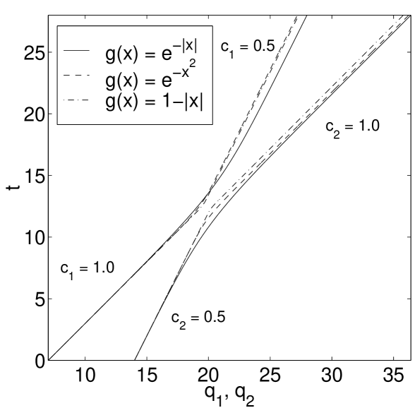
Figure 2.1: Space-time trajectories $q_{1}(t)$ and $q_{2}(t)$ for three typical Green’s functions. For any spatially confined Green’s function, these space-time plots become linear, asymptotically in time. Note that the relative separation $q=q_{2}-q_{1}$ remains positive, so the particles retain their order.

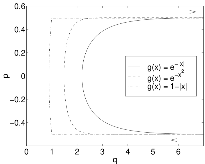
Figure 2.2: Phase space trajectories $p(t)$ vs $q(t)$ of rear-end collisons for three typical Green’s functions. For rear-end collisons these trajectories are nonsingular. Note that $p=p_{2}-p_{1}$ changes sign, while $q=q_{2}-q_{1}$ remains positive; so the particles exchange their momentum, but retain their order.

Head-on pulson-antipulson collision.

For the special case of completely antisymmetric pulson-antipulson collisions, for which $p_{1}=-p_{2}=-p/2$ and $q_{1}=-q_{2}=-q/2$ (so that $P=0$ and $Q=0$) the quadrature formula (2.5) reduces to

$$\pm(t-t_{0})=\frac{1}{\sqrt{4H}}\int_{q(t_{0})}^{q(t)}\frac{dq^{\prime}}{\sqrt{1-g(q^{\prime})}}\,.$$ (2.6)

For this case, the conserved Hamiltonian (2.2) is

$$H=\frac{p^{2}}{4}[1-g(q)]\,.$$ (2.7)

After the collision, the pulson and antipulson separate and travel oppositely apart; so that asymptotically in time $g(q)\to 0$, $p\to 2c$, and $H\to{c}^{2}$, where $c$ (or $-c$) is the asymptotic speed (and amplitude) of the pulson (or antipulson). Setting $H={c}^{2}$ in equation (2.7) gives a relation for the pulson-antipulson $(p,q)$ phase trajectories for any Green’s function,

$$p=\mp\frac{2c}{\sqrt{1-g(q)}}\,.$$ (2.8)

Notice that $1/p$ passes through zero when $q\to 0$, since $g(0)=1$. The relative momentum $p$, initially at $-2c$, diverges to $-\infty$ at the “bounce” collision point as $q\to 0^{+}$. Then $p$ changes sign, $q$ increases again and $p$ asymptotes to $2c$ from above. Thus, $p$ diverges as $q\to 0^{+}$ and switches branches of the square root, from negative to positive. Note also that $q>0$ throughout, so the particles retain their order. The phase space trajectories of head-on collisions for three typical Green’s functions are shown in Figure 2.3.

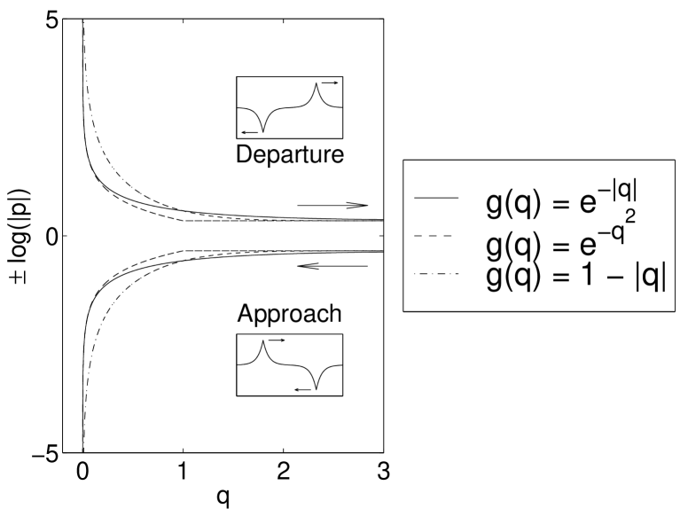
Figure 2.3: Phase space trajectories of head-on collisions for three typical Green’s functions. As $q\to 0^{+}$ at the collison point, $1/p$ passes through zero. Note that $q$ remains positive throughout the collision, so the particles retain their order. In particular, they do not “pass through” each other.

In terms of relative momentum and separation, $p$ and $q$, the solution (1.16) for the velocity $u$ in the head-on pulson-antipulson collision becomes

$$u(x,t)=\frac{-p}{2}g(x+q/2)+\frac{p}{2}g(x-q/2)\,.$$ (2.9)

Using equation (2.8) to eliminate $p$ allows this solution to be written as a function of position $x$ and the separation between the pulses $q$ for any pulse shape $g(x)$ as

$$u(x,q)=\frac{\mp{c}}{\sqrt{1-g(q)}}\Big{[}g(x+q/2)-g(x-q/2)\Big{]},$$ (2.10)

where $c$ is the pulson speed at sufficiently large separation and the dynamics of the separation $q(t)$ is given implicitly by equation (2.6) with $\sqrt{4H}=2c$. Equation (2.10) is the exact analytical solution for the pulson-antipulson collision.

3 Numerical Simulations

We shall summarize our choices of Green’s functions and briefly discuss the numerical method used to compare their pde interaction dynamics in numerical simulations. These numerical simulations demonstrate the qualitative similarity in solution behavior for these Green’s functions in both rear-end (2-pulson) and head-on (pulson-antipulson) collisions. The numerical results show that the dynamics of the initial value problem is dominated by Green’s function wave forms that collide elastically with each other and sort themselves according to height, as solitons do. The reversibility of the numerical dynamics for the initial value problem is also shown, by demonstrating that the dynamics of a set of separated peaked solitary waves may be reversed to reconstruct a smooth initial distribution.

3.1 Choice of Green’s Functions

The choice $g(x)=e^{-|x|}$ satisfies $(1-\partial^{2})g(x)=2\delta(x)$, for which the Hamiltonian (1.3) becomes

$$H_{1}=\frac{1}{2}\int mu\,dx=\frac{1}{2}\int(u^{2}+u^{2}_{x})dx\,.$$ (3.1)

This is the $H_{1}$ norm which generates the peakon dynamics studied in [8], [9], [17], [18]. It is natural to consider higher-derivative norms of this type, such as

$$H_{s}=\frac{1}{2}\int(u^{2}+u^{2}_{s})dx\,,$$ (3.2)

with $u_{s}=\partial^{s}{u}/\partial{x^{s}}$. The corresponding normalized Green’s function

$$g^{(s)}(x)=\frac{1}{R}\sum_{j=0}^{s-1}r_{j}e^{-r_{j}|x|}\,,$$ (3.3)

with $r_{j}=exp\left(\frac{i\pi}{s}\left(j-\frac{s-1}{2}\right)\right)$, $j=0,...,s-1$ and $R=\sum_{j=0}^{s-1}r_{j}$, satisfies

$$\left(1+(-\partial^{2})^{s}\right)g^{(s)}(x)=\frac{2s}{R}\delta(x)\,.$$ (3.4)

The Green’s function $g^{s}(x)$ has a discontinuity in its s-th derivative. The pulse shape (3.3) is plotted for $s=1$ peakons and $s=2,3$ pulsons in Figure 3.1.

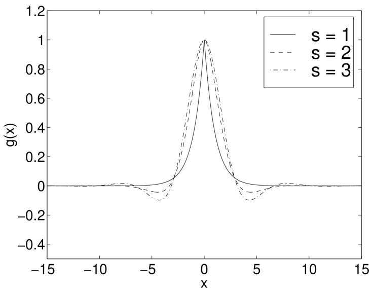
Figure 3.1: Pulson shapes for s=1,2, and 3.

In the high wave number limit, the Hamiltonian (3.2) becomes

$$H_{s,k\rightarrow\infty}=\frac{1}{2}\int u^{2}_{s}\,dx\,,$$ (3.5)

whose corresponding Green’s function satisfies

$$(-\partial^{2})^{s}g_{c}^{(s)}(x)=2s\delta(x)\,.$$ (3.6)

The Green’s functions corresponding to (3.6) having compact support are given by

$$g_{c}^{(s)}(x)=\left\{\begin{array}[]{cl}1+\frac{s(-1)^{s}}{(2s-1)!}x^{2s-1}\hbox{sgn}(x)&\mbox{if $|x|<\left(\frac{(2s-1)!}{s}\right)^{\frac{1}{2s-1}}$}\,,\\ 0&\mbox{otherwise}.\end{array}\right.$$ (3.7)

These are depicted in Figure 3.2 according to (3.7) for $s=1,3$, but the opposite convexity is chosen for $s=2$. These “compacton” Green’s functions serve as examples of traveling wave solutions to (1.1) with compact support.

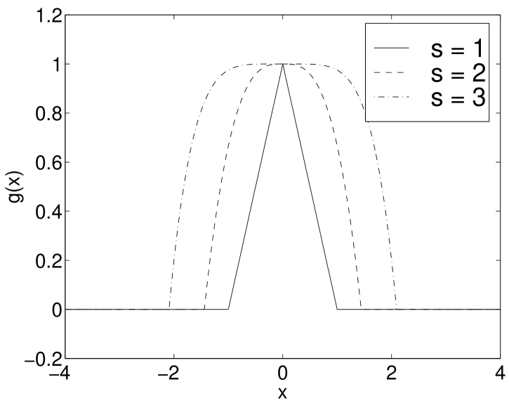
Figure 3.2: Compacton shapes for s=1,2, and 3. These shapes widen as $s$ increases.

In addition to the aformentioned Green’s functions, we also test a Gaussian and a composite Green’s function consisting of one central $s=2$ compacton and two outlying $s=1$ compactons.

3.2 Numerical Method

Equation (1.1) is advanced in time with a fourth order Runge Kutta scheme whose time step is chosen (by numerical trial and error) so as to ensure less than a 1% drop in amplitude over 8 periodic domain traversals. We keep track of the evolution of the Fourier modes of $m(x,t)$ and compute the spatial derivatives in (1.1) pseudospectrally. To transform between $u(x,t)$ and $m(x,t)$ we convolve $m(x,t)$ with the Green’s function in Fourier space as $\hat{u}_{n}=N\hat{g}_{n}\hat{m}_{n}$, where $N$ is the number of Fourier modes, which is kept at 2048 for each run. This method of transforming between $m$ and $u$ proves convenient for arbitrary Green’s functions because the transformation can be computed numerically and the relationship between $m$ and $u$ does not need to be determined explicitly. Because antisymmetric perturbations to the zero solution are unstable [8], [9], and the numerical approximation of the nonlinear terms have aliasing errors in the high wave numbers, we apply the following high pass filtered artificial viscosity [24]

$$\nu(k)=\left\{\begin{array}[]{cl}0&\mbox{if $|k|<\frac{5N}{16}$}\\ 2\varepsilon(\frac{4|k|}{N}-1)&\mbox{if $\frac{5N}{16}<|k|<\frac{3N}{8}$}\\ \varepsilon&\mbox{if $|k|>\frac{3N}{8}$}\end{array}\right.,$$ (3.8)

where $\varepsilon=0.01$ for the present simulations.

3.3 Initial Value Results

Beginning with a normalized Gaussian distribution $u(x,0)=\frac{1}{\sigma\sqrt{\pi}}e^{-{(x-x_{0})^{2}}/{\sigma^{2}}}$ we first show the behavior of the initial value problem for the integrable cases of peakons and $s=1$ compactons. From [8][9], the asymptotic speeds of the emergent integrable pulses can be determined as the eigenvalues of the Sturm-Liouville problem

$$\psi_{xx}-\left[\frac{\delta_{CH}}{4}-\frac{1}{2\lambda}m(x,t)\right]\psi=0,$$ (3.9)

where $m(x,t)$ is the momentum density associated with the velocity of the initial distribution and $\delta_{CH}$ is $1$ for the peakons and $0$ for the $s=1$ compactons. Camassa et al. [9] solve (3.9) analytically with $m(x,0)=A\hbox{sech}^{2}(x)$. The relation of equation (3.9) to the spectral problem for the Schrödinger equation in the case of positive “potential,” $m(x,t)$ has recently been discussed in Beales et al. [25]. See also Constantin [26] for a similar discussion of the spectral problem for equation (3.9) in the periodic case.

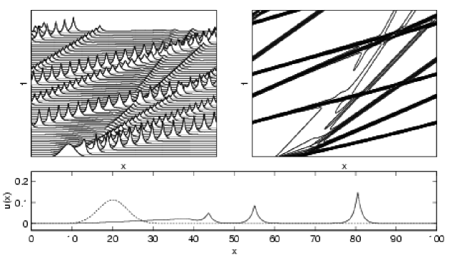
Figure 7.1: $s=1$ peakons emerging from a Gaussian of unit area and $\sigma=5$ centered about $x=20$ on a periodic domain of length $L=100$. A secondary peakon emerges in the upper right hand corner of the contour plot as the faster peakons recross the domain and interact with the residual distribution.

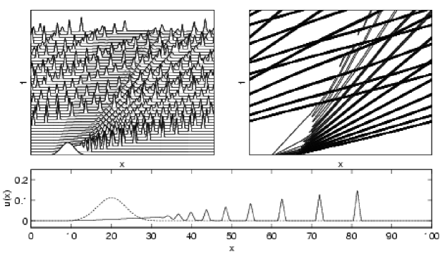
Figure 7.2: $s=1$ compactons emerging from a Gaussian of unit area and $\sigma=5$ centered about $x=20$ on a periodic domain of length $L=100$. More compactons emerge here than peakons in Figure 7.1, because the compactons have smaller area. The residual distribution around $x=20$ causes the space-time trajectories to curve as the larger, faster $s=1$ compactons interact with the slower ones that comprise the residual.

In the simulations we investigate here the asymptotic speeds are given by the heights of the emergent pulses computed numerically from (1.1). Figures 7.1 and 7.2 depict the emergence of peakons and $s=1$ compactons from the initial Gaussian distribution. The integrable behavior is evidenced as the pulses in both cases collide elastically as they recross the periodic domain. Note the presence of roughly nine distinct $s=1$ compactons in Figure 7.2 versus three peakons in Figure 7.1. While the maximum speed is identical for both cases, the number of emergent pulses increases for pulses of smaller area.

In Figure 7.1 we see the interaction of the larger peakons with the slower residual distribution that is left behind by the initial distribution after some early evolution has occurred. Notice that the last two peakons emerging in the upper right hand corner of the contour plot experience a positive phase shift (to the right) shortly after the sixth peakon emerges. This is consistent with the increase in amplitude of the peakon as it grows out of the initial distribution and propagates away, enhanced by the interaction of the larger, faster peakons with the much slower residual distribution, whose peakon content has not yet emerged. This rather complex interaction in which the sixth peakon experiences a significant amount of growth as it traverses the upper right hand corner of the figure could have been avoided by removing the residual distribution remaining after the first few peakons had emerged. However, the Gaussian initial distribution for this figure is comprised of a countable infinity of peakons interacting nonlinearly among themselves. Thus, removing the residual distribution this way would alter the intended initial value problem perhaps unacceptably. Should we desire only a certain finite number of peakons, say, six of them, to emerge from an initial distribution, then we could use the inverse problem to determine what initial distribution is formed from this number of pulses. We discuss the inverse problem as well as the reversible nature of equation (1.1) later in the paper.

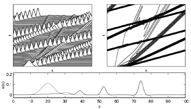
Figure 7.3: $s=2$ pulsons emerging from a Gaussian of unit area and $\sigma=5$ centered about $x=20$ on a periodic domain of length $L=100$. The space-time trajectories curve just after the $s=2$ pulsons emerge from the initial distribution because their large width enhances their interaction range. Note the phase shift in the space-time plot occurring at the trailing edge of the residual distribution as the larger, faster pulsons recross the domain.

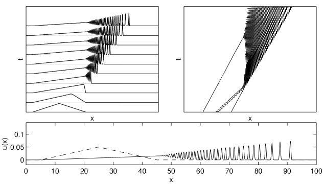
Figure 7.6: Gaussons emerging from an initial $s=1$ compacton of unit area and width $40$ centered about $x=20$ on a periodic domain of length $L=100$. In an effort to avoid confusion, the Gaussons are not shown recrossing the domain.

Next, we discuss the nonintegrable results in Figures 7.3, 7.4, 7.5 and 7.6. In Figure 7.3 we see $s=2$ pulsons emerging from an initial Gaussian velocity distribution. Note the curvature of the space-time trajectories in the contour plot for the third and fourth pulsons. This occurs because the larger width of the $s=2$ pulsons compared to the peakons in Figure 7.1 implies a longer interaction period between pulson pairs. Again we see the effects of the interaction of the larger pulsons with the residual distribution as they recross the periodic domain. Most notably we see the continued emergence of pulsons on the “upwind” side of the initial distribution, leading to the emergence of a pulson at the top center of the contour plot in Figure 7.3. Figures 7.4 and 7.5 also depict this phenomenon of curvature in the space-time trajectories during the emergence of the $s=2$ compactons and Gaussons. In Figure 7.4 the curvature in the space-time trajectories is not only because of the prolonged interaction between the $s=2$ compactons, but also because of their interaction with the residual initial distribution as they recross the domain. We do not show the Gaussons emerging from the initial $s=1$ compacton shape and colliding with the initial residual distribution in Figure 7.6 because there are too many pulses to make a clear plot. However, this figure helps to support our main conclusion: that an arbitrary (even) wave form given by the Green’s function $g(x)$ can be made to emerge from an (essentially) arbitrary confined initial condition. In this case we have chosen a wide $s=1$ compacton for the initial distribution partly because its shallow discontinuity imposes less stringent conditions on the numerics, and also to demonstrate the effects that the width of the initial condition has on the number of emergent pulses. Namely, the width of the initial distribution must be greater than the single pulson width prescribed by the function $g(x)$, and wider initial distributions produce a larger number of pulsons.

In summary, Figures 7.3, 7.4, 7.5 and 7.6 demonstrate that: (1) the shape of each wave form emerging in the initial value problem is controlled by the choice of $g(x)$; and (2) the dynamical behavior of the emergent pulses is qualitatively the same as the integrable behavior of the peakons and $s=1$ compactons.

3.4 Rear-End Collisions

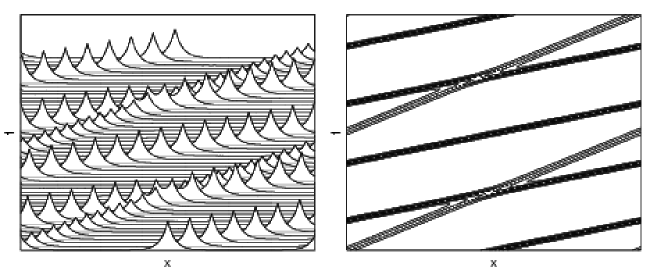
Figure 7.7: Rear-end collision dynamics for $s=1$ peakons. The faster peakon moves at twice the speed of the slower one. For this case, both collisions result in a phase shift to the right for the faster space-time trajectory, but no phase shift for the slower one. The phase shift causes the second collision to occur slightly to the left of the first.

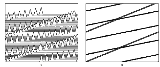
Figure 7.8: Rear-end collision dynamics for $s=1$ compactons. The faster space-time trajectory experiences a phase shift to the right while the slower one experiences a phase shift to the left.

We compute the evolution governed by equation (1.1) with two wave forms (for a particular choice of Green’s function) located initially at $x=0$ and $x=L/2$ with amplitudes $c_{1}=1$ and $c_{2}=1/2$, respectively. This situation is arranged to investigate the nature of rear-end collisions both for the integrable and nonintegrable cases. Beginning with the integrable cases depicted in Figures 7.7 and 7.8, we see that, consistent with the findings of [9], the slower peakon in Figure 7.7 experiences no phase shift, but the faster peakon experiences a shift to the right. This occurs after each collision, thus causing the second collision to occur to the left of the first. In Figure 7.8 we see that the faster $s=1$ compacton trajectory experiences a phase shift to the right while the slower one experiences a shift to the left. Thus, perhaps not unexpectedly, the phase shift of the interaction depends on the pulse shape. The sudden leftward phase shift of the slower trajectory indicates that momentum is being transferred rightward rather quickly in the collision process across the entire width of both wave forms. This is something like the sudden transfer of momentum in the collision of billiard balls. For this reason, the magnitude of the phase shift increases with pulse width. Note that the pulsons exchange momentum in each collision, rather than passing through each other.

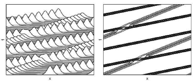
Figure 7.9: Rear-end collision dynamics for $s=2$ pulsons. The faster space-time trajectory experiences a phase shift to the right while the slower one experiences a phase shift to the left. The size of the interaction region is proportional to the sum of the pulse widths.

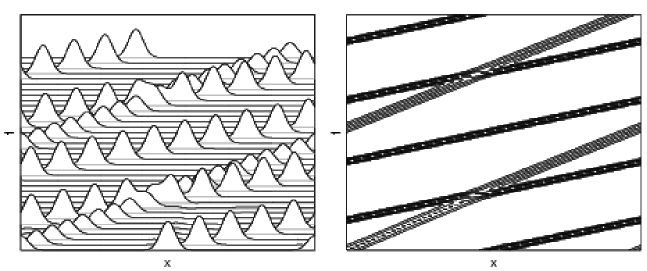
Figure 7.11: Rear-end collision dynamics for Gaussons. The faster space-time trajectory experiences a phase shift to the right while the slower one experiences a phase shift to the left. Because they are so narrow, Gaussons have the smallest phase shift of the four nonintegrable cases depicted in this figure and Figures 7.9, 7.10, and 7.12.

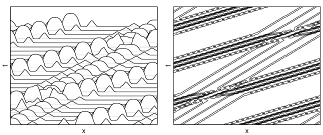
Figure 7.12: Rear-end collision dynamics for multicompactons. The faster space-time trajectory experiences a phase shift to the right while the slower one experiences a phase shift to the left. The large width and hence large interaction range of the multicompactons causes them to have the largest phase shift of the four nonintegrable cases depicted in this figure and Figures 7.9, 7.10, and 7.11.

The nonintegrable cases depicted in Figures 7.9, 7.10, 7.11, and 7.12 all show similar elastic collisions resulting only in phase shifts. In each case the faster pulse trajectory experiences no shift, or a shift to the right, while the slower one experiences a shift to the left. The magnitude of the shift increases with pulse width. The pulse width is the largest for the multicompactons in Figure 7.12 and they experience the largest phase shift of the four nonintegrable cases shown here. The Gaussons in Figure 7.11, on the other hand, experience the least phase shift and they are the narrowest of the four nonintegrable pulsons we treat.

3.5 Head-on Collisions

We use the exact solution $u(x,q)$ for arbitrary Green’s functions in equation (2.10) to determine the velocity profiles in head-on antisymmetric pulson-antipulson collisions. The complexity of the wave shapes and the strengths of the various singularities which form according to equation (2.10) during these interactions for many choices of pulson shapes are beyond the capabilities of most numerics. For example, the spatial derivative of equation (2.10) at $x=0$ gives

$$u_{x}(0,q)=\frac{2c}{\sqrt{1-g(q)}}g^{\prime}(q/2)\,.$$ (3.10)

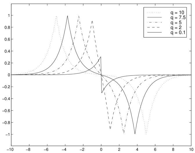
Figure 7.13: Head-on collision dynamics for $s=1$ peakons at five pre-collision separations $q$. The velocity tends to zero as the separation between the peakons tends to zero and a verticality in slope develops at $x=0$, as $q\to 0^{+}$. At this collision point, the solution reverses its polarity by flipping across the horizontal axis (so that $u\to-u$) and the peakons move apart in opposite directions.

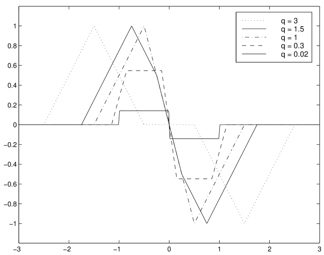
Figure 7.14: Head-on collision dynamics for $s=1$ compactons at five pre-collision separations $q$. As the compactons meet, the slope at $x=0$ remains at $u_{x}(0,q)=-2$ until their peaks are clipped when $q=1$. Thereafter the slope at $x=0$ begins to increase and eventually becomes vertical when $q=0$ just as the velocity vanishes. At this moment the solution reverses polarity and the compactons re-emerge, moving apart in opposite directions.

Hence, whether a vertical slope in $u$ forms at $x=0$ depends on the choice of the Green’s function $g(x)$. Colliding peakon-antipeakon profiles are depicted in Figure 7.13. As discussed in [9] the solution $u$ in this case tends to zero as $q\rightarrow 0$, as the slope $\lim_{q\to 0}u_{x}(0,q)$ diverges to minus infinity. Also, $p\rightarrow\infty$ as $q\rightarrow 0$, so as to maintain constant energy and zero total momentum in the particle system. This divergence phenomenon occurs similarly for the $s=1$ compactons, as shown in Figure 7.14.

As with the peakons, the colliding $s=1$ compactons develop a vertical slope in velocity at $x=0$ when $q~{}=~{}0$. Upon making initial contact when $q=2$, the two triangular pulses develop a maximum negative slope at $x=0$ of $u_{x}(0,q)|_{q\in[1,2]}=-2c$ which remains constant until $q=1$, whereupon the two pulses begin to clip their peaks and become trapezoidal as the slope at $x=0$ tends toward minus infinity via $\lim_{q\to 0^{+}}u_{x}(0,q)=-2c/\sqrt{|q|}$, cf. equation (3.10). When $q=0$, the two colliding pulses diminish to $u=0$ and then “bounce” apart to reverse the aformentioned process, so that $u_{x}(0,q)=+2c/\sqrt{|q|}$ until $q=1$ with $u_{x}(0,q)|_{q\in[1,2]}=+2c$. Thereafter, the reformed pulses separate in opposite directions. Note that $q$ approaches zero, but does not change sign; so the “particles” with phase space coordinates $p_{i}$, $q_{i}$, $i=1,2$, keep their order, just as for the rear-end collisions.

The most significant difference between the integrable and nonintegrable pulson-antipulson collisions is that the solution $u(x,q)$ does not necessarily tend toward zero as $q\rightarrow 0$ for the nonintegrable cases. Another difference is that a verticality in slope does not necessarily develop at $x=0$. Moreover, such a verticality may not develop at all. As an example of a nonintegrable pulse that does not approach $u=0$ as $q\to 0$, but does develop two verticalities at that instant, we consider a parabolic pulse such that

$$g(x)=\left\{\begin{array}[]{cl}1-x^{2}&\mbox{if $|x|\leq 1\,,$}\\ 0&\mbox{otherwise}.\end{array}\right.$$ (3.11)

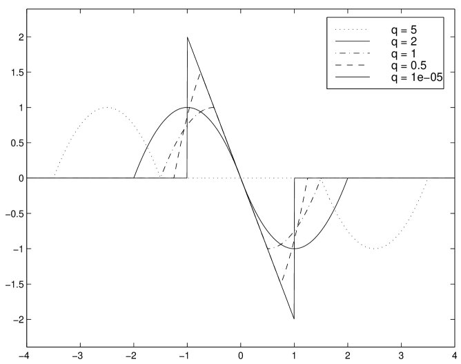
Figure 7.15: Head-on collision dynamics for parabolas at five pre-collision separations $q$. Parabolas collide to form a finite distribution when $q=0^{+}$ and two verticalities in slope appear at $x=\pm 1$. After the collision the solution reverses polarity and the parabolas move apart, preserving the antisymmetry.

The antisymmetrically colliding parabolas are shown in Figure 7.15. As the parabolic pulson collides with its antipulson, two verticalities develop at $x~{}=~{}\pm~{}1$ rather than at $x=0$. By equation (2.10), this interaction creates a limiting distribution such that

$$\lim_{q\rightarrow 0^{+}}u(x,q)=\left\{\begin{array}[]{cl}-2cx&\mbox{if $|x|\leq 1\,,$}\\ 0&\mbox{otherwise}.\end{array}\right.$$ (3.12)

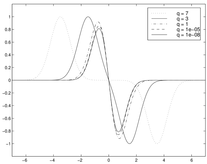
Figure 7.16: Head-on collision dynamics for Gaussons at five pre-collision separations $q$. Gaussons collide to form a finite distribution when $q=0^{+}$ and develop no verticalities in slope. After the collision the solution reverses polarity and the Gaussons move away from each other.

As an example of a nonintegrable pulson that does not tend toward $u=0$ and develops no verticalities in slope as $q\rightarrow 0$, we consider the antisymmetrically colliding Gaussons depicted in Figure 7.16. Here the limiting distribution is

$$\lim_{q\rightarrow 0^{+}}u(x,q)=-2cxe^{-x^{2}}.$$ (3.13)

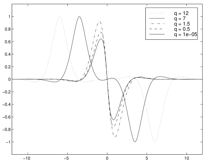
Figure 7.17: Head-on collision dynamics for $s=2$ pulsons at five pre-collision separations $q$. As for the Gaussons in Figure 7.16, $s=2$ pulsons collide to form a finite distribution when $q=0^{+}$ and develop no verticalities in slope. At the moment of collision, the solution reverses polarity and then the $s=2$ pulsons move apart antisymmetrically.

When an antisymmetric collision results in a limiting distribution as in equations (3.12) and (3.13) as $q\rightarrow 0^{+}$, the solutions must flip instantaneously as they approach $q=0^{+}$, and bounce apart so that the post-collision interaction will be identical but opposite in polarity to the pre-collision interaction. This situation also occurs similarly for the antisymmetric collision of $s=2$ pulsons, shown in Figure 7.17. However, the analytical solution for the limiting $q\rightarrow 0^{+}$ distribution is not so easily expressed in this case, so we omit it here.

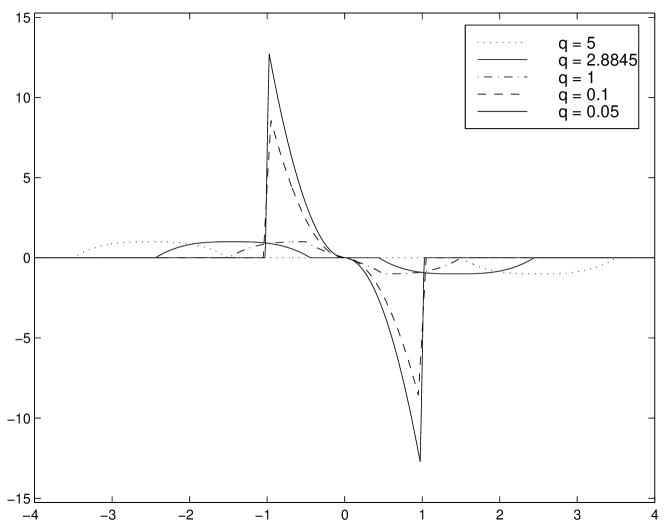
Figure 7.18: Head-on collision dynamics for $s=2$ compactons at five pre-collision separations $q$. The $s=2$ compactons collide to form two verticalities in slope at $x=\pm 1$ as well as unbounded growth in $u(x,q)|_{x=\pm 1}$ as $q\to 0+$. At this moment, the solution reverses polarity and the compactons move apart in opposite directions.

An even more complex situation develops when two $s=2$ compactons collide antisymmetrically, as shown in Figure 7.18. In this case, not only do the colliding pulses develop two verticalities, but there is no limiting distribution as $q\rightarrow 0^{+}$. In fact, one can show for $s=2$ compactons (with the factor of $1/3$ omitted for convenience) that

$$u(x=\pm 1,q)=\mp\frac{2}{\sqrt{q}}\left(1+\frac{q^{2}}{8}\right),$$ (3.14)

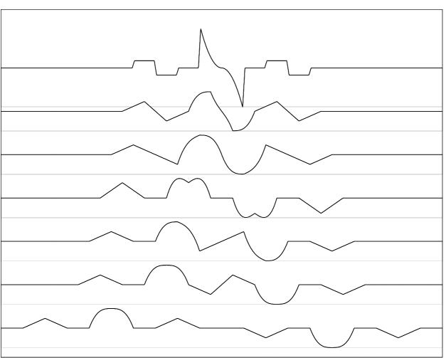
Figure 7.19: Head-on collision dynamics of multicompactons depicted at separations of $q=$ 10, 5, 4, 3, 2, 1, and 0.1. We avoid confusion and show a “waterfall” plot to depict the multicompactons rather than an overlay. Here, verticalities as well as unbounded growth in $u(x,q)$ develop at $x=\pm 1$, $\pm 2$, $\pm 3$, and $\pm 4$ as $q\to 0^{+}$. The last distribution is scaled by a factor of $1/2$ to keep the large amplitudes resulting from the approaching unboundedness of $u(x,q)$ within the plot.

so that the velocity at $x=\pm 1$ becomes unbounded as $q\rightarrow 0^{+}$. However, as soon as $q$ reaches zero, the unbounded solution for $u$ switches sign and the pulses restore themselves with reversed polarity and move apart. As a final example we show in Figure 7.19 the antisymmetric collision of “multicompactons,” again with the factor of $1/3$ omitted from the central hump for convenience. Here we use a “waterfall” plot to depict the collision since an overlay would be too confusing. This collision results in the creation of eight verticalities at $x=\pm 1$, $\pm 2$, $\pm 3$, and $\pm 4$. Again, as $q\to 0^{+}$, the solution flips polarity instantaneously and the interaction reverses as the multicompactons move apart.

3.6 Reversibility

The results in Section 3.3 for the initial value problem show that a train of pulses in the prescribed pulse shape $g(x)$ emerges from any initial distribution and dominates the initial value problem. In this process, the initial distribution breaks up into a discrete number of pulsons, each of which travels at a speed equal to its height, and the pulsons collide elastically among each other as they recross the periodic domain. An interesting feature of equation (1.1) is that it is time reversible, that is, invariant under $t\to-t$ and $u\to-u$. Thus, replacing $dt$ with $-dt$ at any point in the numerical simulations causes the pulsons emerging in the initial value problems to reverse their evolution sequence (but not their heights) and collapse together into the initial distribution. Thus the time-reversed series of collisions reforms the original initial distribution at $t=0$. This process enables us in principle to determine the parameters $p_{i}$, $q_{i}$, $i=1,\dots,N$, on the invariant manifold by running the pde (1.1) forward in time until $N$ pulsons have emerged, then reversing the solution to recreate the original smooth initial distribution. Similarly, we may run the pde forward until time $T$, determine the parameters ($p_{i},q_{i}$) at this time, remove any residual velocity distribution from which pulsons have not yet emerged, then time-reverse the ordinary differential equation (ode) dynamics for a period $T$ to create an initial distribution containing only the pulson content that will emerge before time $T$. Should this process, denoted in obvious notation as $[ODE(-T)\circ\Pi_{N}\circ PDE(T)]u(x,0)$, produce an accurate approximation $u_{N}(x,0)$ of the original distribution $u(x,0)$, it would be a useful procedure for approximately determining the pulson invariant manifold content of a given initial velocity distribution.

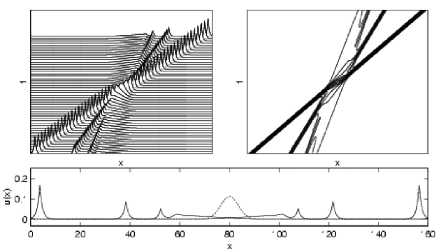
Figure 7.20: $s=1$ peakons colliding to form a Gaussian and then reemerging symmetrically thereafter.

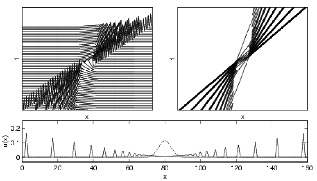
Figure 7.21: $s=1$ compactons colliding to form a Gaussian and then reemerging symmetrically thereafter.

Figures 7.20 and 7.21 were constructed by running the pde forward in time from an initial Gaussian distribution until trains of three peakons in Figure 7.20 and nine $s=1$ compactons in Figure 7.21 emerged. At this point time was reversed, and the pde was run in reverse for twice as long, then the solution was reflected in space. In this process trains of pulsons in reversed order (with the tallest ones behind) reassembled moving rightward into the original initial condition and then re-emerged as before (with the tallest ones ahead). The same “geodesic pulson scattering” figures could be generated by running the initial Gaussian distribution both forward and backward in time, then superposing the results. Formally we have $S(t)R_{x}S(t)=Id$ (where $S(t)$ is pde evolution for time $t$ and $R_{x}$ is reflection in space), for initial conditions that are symmetric about the origin. Thus these figures could also have been generated by the process of evolution, reflection, then evolution again. This time reversal symmetry property indicates that the initial distribution may be regarded not just as a sum of pulsons, but as a moment in time at which a set of pulsons moving geodesically has collided to form a smooth distribution, in this case a Gaussian.

4 Conclusions

In equations (1.1) and (1.2) we have introduced a new family of hyperbolic pde describing a certain type of geodesic motion and for some members of this family we have studied its particle-like solutions. We call these solutions “pulsons.” We have shown that, once initialized on their invariant manifold (which may be finite-dimensional), the pulsons undergo geodesic dynamics in terms of canonical Hamiltonian phase space variables. This dynamics effectively reproduces the classical soliton behavior. We conjecture that this behavior occurs because of the preponderance of two-body elastic-collision interactions for the situation we consider of confined pulses and confined initial conditions.

The dynamics we study in this framework of geodesic motion on a finite-dimensional invariant manifold seems to account for all of the classical soliton phenomena, including elastic scattering, dominance of the initial value problem by confined pulses and asymptotic sorting according to height – all without requiring complete integrability. Thus, complete integrability is apparently not necessary for exact soliton behavior. Regarding the “formation” of the pulsons: in fact, the pulsons must always be present, since they compose an invariant manifold. One discerns them in a given (confined) initial condition by using the isospectral property in the integrable cases, or just by waiting for them to emerge under the pde dynamics in the nonintegrable cases. However, there is no “pattern formation” process in this dynamics. Rather, there is an “emergence of the pattern,” which is the pulson train.

This conclusion is illustrated by Figures 7.20 and 7.21 showing geodesic scattering of an incoming set of pulsons that collapses into a smooth “initial” distribution, then fans out again into an outgoing set of pulsons that is the mirror image of the incoming set. This parity-reflection is an implication of reversibility, as well; since reversing the dynamics of a set of separated pulsons reassembles them into a smooth “initial” distribution, which is just their sum, with appropriate values for their initial “moduli” parameters $p_{i}(0),q_{i}(0)$, $i=1,\dots,N$. The moduli parameters $p_{i},q_{i}$ are collective phase space coordinates on an invariant manifold for the pde motion. Once initialized, these collective degrees of freedom persist and emerge as a train of pulses, arranged in order of their heights. Moreover, since their velocity is their peak height, small residual errors departing from the pulson superposition in the assignment of initial parameter values $p_{i}(0),q_{i}(0)$, $i=1,\dots,N$, do not propagate significantly. On the real line, such residual errors are simply left behind by the larger pulsons traveling more quickly. And on the periodic interval, these errors provide an occasional phase shift perturbation to the stable pulsons. These perturbations are seen in the figures as regions of curvature in the space-time trajectories of the pulsons.

Our main conclusions regarding the elastic collisions of the pulsons and their role in the pde initial value problem are the following:

1. Two-pulson interactions are elastic collisions that conserve total kinetic energy and transfer momentum, as measured by the asymptotic speeds and peak heights of the pulsons. The motion of the pulsons is governed by geodesic kinematics of particles with no internal degrees of freedom; but with an interaction range, or spatial extent, which is given by their Green’s function, or wave form, $g(x)$. Thus, these interactions are analogous to the collisions of billiard balls. This is especially clear for pulsons of compact support.

2. The exact solution in equation (2.10) determines analytically the complex wave shapes and the strengths of the various singularities that may form during antisymmetric head-on collisions of pulsons and antipulsons. These singularities are verticalities in slope at which the velocity may diverge, take a finite value, or even vanish, depending on the choice of Green’s function. At the moment of collision, the pulson and antipulson “bounce” apart and the polarity of the antisymmetric wave form reverses, $u\to-u$. Again this is analogous to billiards, but with the difference that the reversal of momentum reverses the polarity of the pulson velocity profile. Note that the wave forms reverse polarity and bounce apart; they do not actually “pass through” each other, although they may appear to do so.

3. The dynamics on the pulson invariant manifold is dominated by the preponderance of two-body collisons. To the extent that the initial value problem for the pde takes place on the pulson invariant manifold, these two-pulson collisions should also dominate the solution of the pde dynamics. We conjecture this is so for most choices of confined pulse and initial conditions of finite extent for the family of pde (1.1) with $u$ given in (1.2).

Thus, geodesy governs the motion and explains the elastic-scattering soliton phenomena we observe, without providing (or even requiring there exists) a means of analytically solving the initial value problem for this family of pde. Even the motion on the pulson manifold is not integrable for $N>2$, except in the cases corresponding to the Camassa-Holm, and Dym integrable pde. Similar geodesic but nonintegrable families of equations showing soliton behavior on a finite-dimensional invariant manifold may exist for other integrable geodesic equations, such as KdV.

5 Acknowledgments

This work was supported in part by the Computational Science Graduate Fellowship Program of the Office of Scientific Computing in the Department of Energy. For their kind attention, suggestions and encouragement, we are happy to thank R. Camassa, P. Constantin, P. Fast, C. Foias, I. Gabitov, J. M. Hyman, Y. Kevrekidis, S. Shkoller, P. Swart and S. Zoldi.

6 Appendix on Numerical Stability

As discussed in Section 3.2, we add dissipation in the higher modes for the simulations covered in this paper because the Fourier pseudospectral method used is unstable to perturbations at the grid scale. These perturbations arise as a result of the Gibbs phenomenon which causes an overshoot to occur at points of discontinuous slope in $u$. Such an overshoot forms negative values of the function $u$, which can artificially create antipulsons that emerge and interact with positive pulsons to form verticalities in slope as described in Section 3.5. As an example, we tested the stability of the numerical method by initializing the domain with a perturbation at a single grid point, as

$$u_{i}=\left\{\begin{array}[]{cl}10^{-3}&\mbox{if $i=N/2\,,$}\\ 0&\mbox{otherwise},\end{array}\right.$$ (6.1)

for $i=1,\dots,N$. This initial distribution was unstable and caused exponential growth in the neighboring grid points, such that $u_{N/2-1}\to+\infty$ and $u_{N/2+1}\to-\infty$, resulting from the creation of a pulson-antipulson pair whose peaks grew unstably. We then ran the same initial condition with a dissipation coefficient of $\varepsilon=0.01$ in equation (3.8), which stabilized it. We also ran it again with a nonzero linear dispersion coefficient of $\kappa=0.01$ in equation (1.11) which stabilized it as well. Adding dissipation damps the higher modes as specified in Section 3.2 while adding linear dispersion smooths discontinuities in $u$, thus effectively damping the higher modes. Thus, either dissipation or dispersion will suppress instability due to perturbations at the grid scale.

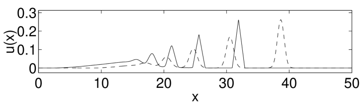
Figure 6.1: $s=1$ compactons emerging from a Gaussian of width $\sigma=3$ and unit area centered about $x=10$ on a periodic domain of length $L=50$ demonstrating the effects of the linear dispersion coefficient $\kappa$. The solid line depicts the $\kappa=0$ case with added dissipation while the dashed line depicts the $\kappa=10^{-3}$ case with no dissipation.

Figure 6.1 compares dissipative and dispersive dynamics for the case of $s~{}=~{}1$ compactons emerging from an initial Gaussian velocity distribution. Linear dispersion ($\kappa\neq 0$) acts to smooth out discontinuities as well as hastening the emergence time of each pulson. This is demonstrated by the separation between the leading pulses for the $\kappa=10^{-3}$ and $\kappa=0$ cases. Despite the negligible difference in speed between the two, the leading $\kappa=10^{-3}$ pulson is far ahead of the leading $\kappa=0$ pulson, because the former was emitted sooner. Stability is acquired by suppressing the higher modes, as shown in Figure 6.2. Here the power spectrum of one compacton is shown for both values of $\kappa$. Introduction of linear dispersion with $\kappa=10^{-3}$ damps the higher modes by roughly three orders of magnitude.

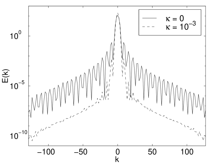
Figure 6.2: Power spectra of one pulse for the $\kappa=0$ and $\kappa=10^{-3}$ cases.

7 Figures

Figure 7.4: $s=2$ compactons emerging from a Gaussian of unit area and $\sigma=5$ centered about $x=20$ on a periodic domain of length $L=100$. The space-time trajectories curve slightly as they emerge from the initial distribution and then straighten out when the compactons are no longer interacting. The space-time trajectories curve again as the compactons recross the domain and interact with the residual distribution.

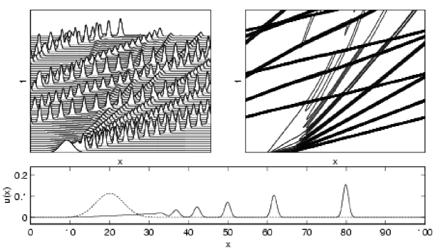
Figure 7.5: Gaussons emerging from an initial Gaussian of unit area and $\sigma=5$ centered about $x=20$ on a periodic domain of length $L=100$. The interaction of the faster Gaussons with the residual “ramp” distribution causes another Gausson to emerge at the top center of the contour plot. The interaction between nearby Gaussons and between Gaussons and the residual distribution causes their space-time trajectories to curve.

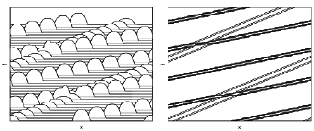
Figure 7.10: Rear-end collision dynamics for $s=2$ compactons. The faster space-time trajectory experiences a phase shift to the right while the slower one experiences a phase shift to the left.

References

- [1] H. Poincaré, Sue une forme nouvelle des équations de la méchanique. C. R. Acad. Sci., Paris, 132 (1901) 369-371.
- [2] V.I. Arnold, Sur la géométrie differentielle des groupes de Lie de dimenson infinie et ses applications à l’hydrodynamique des fluids parfaits. Ann. Inst. Fourier, Grenoble 16 (1966) 319-361.
- [3] J.E. Marsden and T.S. Ratiu, Introduction to Mechanics and Symmetry. Texts in Applied Mathematics 17, Springer, New York (1994).
- [4] D.D. Holm, J.E. Marsden, and T.S. Ratiu, Euler-Poincaré equations and semidirect products with applications to continuum theories. Adv. in Math., 137 (1998) 1-81.
- [5] V.Y. Ovsienko and B.A. Khesin, Korteweg-de Vries superequations as an Euler equation. Funct. Anal. Appl. 21 (1987) 329-331.
- [6] G. Segal, The geometry of the KdV equation. Int. J. Mod. Phys. A 132 (1991) 2859-2869.
- [7] G. Misiolek, A shallow water equation as a geodesic flow on the Bott-Virasoro group. J. Geom. Phys., 24 (1998) 203-208.
- [8] R. Camassa and D.D. Holm, An integrable shallow water equation with peaked solitons. Phys. Rev. Lett. 71 (1993) 1661-1664.
- [9] R. Camassa, D.D. Holm and J.M. Hyman, A new integrable shallow water equation. Advances in Applied Mechanics, Academic Press: Boston, vol 31 (1994) 1-33.
- [10] D.D. Holm, J.E. Marsden, and T.S. Ratiu, Euler–Poincaré models of ideal fluids with nonlinear dispersion. Phys. Rev. Lett., 80 (1998) 4173-4177.
- [11] S. Shkoller, Geometry and curvature of diffeomorphism groups with metric and mean hydrodynamics. J. Func. Anal., (1998) to appear.
- [12] D.D. Holm, S. Kouranbaeva, J.E. Marsden, T. Ratiu and S. Shkoller, A nonlinear analysis of the averaged Euler equations, Fields Inst. Comm., Arnold Vol. 2, Amer. Math. Soc., (Rhode Island), (1998) to appear.
- [13] Y. Brenier, The least action principle and the related concept of generalized flows for incompressible perfect fluids. J. Amer. Math. Soc., 2 (1989) 225-255.
- [14] A.I. Shnirelman, Generalized fluid flows, their approximation and applications. Geom. Func. Anal., 4 (1994) 586-620.
- [15] D.D. Holm, J.E. Marsden and S. Shkoller, Generalized flows of shallow water waves, in preparation.
- [16] J. Hunter and Y. Zheng, On a completely integrable nonlinear hyperbolic variational equation. Physica D, 79 (1994) 361-386.
- [17] M. Alber, R. Camassa, D.D. Holm and J.E. Marsden, The geometry of peaked solitons and billiard solutions of a class of integrable PDE’s. Lett. Math. Phys. 32 (1994) 137-151.
- [18] M. Alber, R. Camassa, D.D. Holm and J.E. Marsden, On the link between umbilic geodesics and soliton solutions of nonlinear PDE’s. Proc. Roy. Soc. 450 (1995) 677-692.
- [19] A. Constantin and H. McKean, A shallow water equation on the circle, Comm. Pure Appl. Math., to appear.
- [20] M.S. Velan and M. Lakshmanan, Lie symmetries and infinite-dimensional Lie-algebras of certain ()-dimensional nonlinear evolution-equations. J. Phys. A 30 (1997) 3261-3271.
- [21] Each member of the hierarchy of equations for powers of resulting from (1.4) possesses a measure-valued traveling wave solution similar to (1.15). However, we shall concentrate on solutions of this type for equation (1.1).
- [22] F. Calogero, An integrable Hamiltonian system. Phys. Lett. A 201 (1995) 306-310.
- [23] F. Calogero and J.P. Francoise, A completely integrable Hamiltonian system. J. Math. Phys. 37 (1996) 2863-2871.
- [24] J. M. Hyman, personal communication.
- [25] R. Beales, D. H. Sattinger, and J. Szmigielski, Acoustic Scattering and the Extended Korteweg deVries Hierarchy. (1998) preprint.
- [26] A. Constantin, On the inverse spectral problem for the Camassa-Holm equation. J. Funct. Anal. 155 (1998) 352-363.