A zero-field Ising model with ferromagnetic coupling constants on the so-called Labyrinth tiling is investigated. Alternatively, this can be regarded as an Ising model on a square lattice with a quasi-periodic distribution of up to eight different coupling constants. The duality transformation on this tiling is considered and the self-dual couplings are determined. Furthermore, we analyze the subclass of exactly solvable models in detail parametrizing the coupling constants in terms of four rapidity parameters. For those, the self-dual couplings correspond to the critical points which, as expected, belong to the Onsager universality class.

1 Introduction

The understanding of phase transitions in 2D systems has considerably increased during the last decade. In particular, a lot is known about the conformal structure at the critical point of a whole hierarchy of models [2]. On the other hand, numerous series of solvable vertex models [3, 4] and IRF (Interaction-Round-a-Face) models [3, 5] have been constructed. Furthermore, the so-called chiral Potts models [6, 7] attracted a lot of interest, mainly due to the existence of superintegrable cases [6] (see also [8] and references therein) and applications to 3D systems [9].

While many of these models can be solved in the presence of a temperature-like deviation from criticality, solvability is in general restricted to the zero-field case (apart from e.g. the hard hexagon model [3] which is a limiting case of the triangular Ising model in a symmetry-breaking field). Recently, a series of models which can be solved in the presence of a symmetry breaking “field” was found [10], among them a model which belongs to the universality class of the Ising model in a magnetic field. But even on regular lattices, notably the square lattice, the word “solvable” does not mean that all physically interesting quantities have been calculated explicitly, in particular the computation of two-point (or even higher) correlation functions still appears to be a hopeless task in the general case.

Even less, however, is known about models on non-periodic graphs. The main reason is that quite a number of new phenomena show up: already the Lee-Yang zeros of the classical 1D Ising model on substitution chains reveal gap structures that are unknown in the periodic case [11]. Similarly, the Ising quantum chain on such substitution structures [12, 13, 14, 15] and the 2D Ising model with aperiodicity in one direction [16, 17] resemble the periodic situation at its critical point only under special conditions. These examples also show that results from conformal field theory cannot generally be applied to systems on non-regular graphs which is not too surprising as they rely on the basic assumption of conformal invariance of the system at the critical point.

The restricted knowledge about non-periodic systems is due to the significantly increased difficulty to reach rigorous results, the study of 8-vertex models on relatively general grids [18, 19] or certain IRF models on (rhombic) duals of regular de Bruijn grids [19, 20] being untypical exceptions (see [21] for a definition of the grid formalism). Other investigations make use of various approximative techniques such as, for instance, real space renormalization group [22, 23], mean field calculations [24], computer simulations [25, 26, 27, 28, 29], series expansions [30], and finite-size scaling methods [31], but almost exclusively deal with Ising or Potts models on Penrose tilings.

In this article, we consider the zero-field Ising model defined on a different quasiperiodic graph in 2D. We have chosen the so-called Labyrinth tiling, see [32] for a detailed geometric description. It turns out that this tiling is self-dual as a graph. This allows – under certain assumptions such as uniqueness of the critical point – a simple argument to obtain information about the location of critical points, though it turns out to be incomplete. In the case of the frequently studied Penrose patterns, duality and correlation inequalities are less conclusive, but have been used to obtain bounds for the critical temperature [25, 28].

From the Peierls argument [33, 34, 35] it is clear that there must exist at least one phase transition in our system. We do not expect that the continuous transition in the Ising model on regular lattices becomes a first-order transition in our case since introducing “randomness” generally tends to smooth out transitions, though it is certainly not completely obvious (e.g., the four-spin interaction Ising model on the tetrahedra of the 3D fcc lattice in fact has a first-order transition at its self-dual point [36]).

Unfortunately, we could not decide the question of uniqueness of the critical point in the ferromagnetic case in general, though one might expect this to be true if all coupling constants are strictly positive and uniformly bounded from below. To further attack this problem, we have investigated the solvable cases of the model by means of the rapidity line approach [37]. We find a 4D manifold in the 8D space of couplings where the Ising model on the Labyrinth is solvable. Therein, one finds a 3D critical surface, hence it contains one temperature-like parameter that describes the deviation from criticality. The result is given explicitly by means of some geometric properties of the Labyrinth. In all these cases, the critical point is unique and belongs to the Onsager universality class as expected [38, 39].

2 The Labyrinth tiling

To investigate exactly some typical properties of generic non-periodic graphs in 2D, we need a simple example which is more complicated than the Cartesian product of a Fibonacci chain and a 1D periodic lattice (which is what underlies the well-studied Ising quantum chains), but still considerably simpler than a Penrose tiling. The natural choice is the so-called Labyrinth tiling [32], which got its name from the properties of certain colourings. There exist several ways to construct it, see [32, 40] for a detailed description. For our purpose, an approach via the Cartesian product of a 1D substitution sequence with itself is most appropriate which we will now briefly outline.

2.1 The silver mean substitution rule

Let us start with the generation of a 1D chain, the so-called silver mean chain, by repeated application of the two-letter substitution rule

$$\varrho\,:\,\,\begin{array}[]{rcl}a&\rightarrow&b\\ b&\rightarrow&bab\end{array}$$ (2.1)

to the letter $a$. The corresponding substitution matrix $R$ is obtained from the standard abelianization process, compare [41] and refs. therein, and reads

$$R=\left(\begin{array}[]{cc}0&1\\ 1&2\end{array}\right)\,.$$ (2.2)

The Perron-Frobenius eigenvalue is the silver mean, $\lambda=1+\sqrt{2}$, the corresponding eigenvector reads $(1,\lambda)^{t}$, or $((3-\lambda)/2,(\lambda-1)/2)^{t}$ in statistical normalization. Since $R$ is symmetric, left and right eigenvectors are the transpose of each other. Thus, the entries have two meanings: on the one hand, they tell us the relative frequencies of $a$’s and $b$’s in the infinite chain – the ratio of which is the irrational number $\lambda$ wherefore the chain cannot be periodic. On the other hand, they give us the natural choice for the lengths of two intervals with which we can represent the chain geometrically such that the substitution rule (2.1) gives rise to a inflation/deflation symmetry. In this setup (which we shall use for graphical presentation), $a$ stands for a short interval, while that attached to $b$ is a factor of $\lambda$ longer.

2.2 Construction of the Labyrinth

The next step is to generate a 2D tiling. First, we take an orthogonal Cartesian product of two identical silver mean chains in the proper geometric representation. This way, we obtain a quadrant with an orthogonal grid, but two different spacings in each direction. Now, starting from the lower left corner, we mark every second vertex point of this grid and connect them with the nearest neighbours of the same kind. This would then give a fourfold symmetric, non-periodic tiling of the plane (after filling the 3 free quadrants with rotated copies of the grid constructed).

In what follows, we shall, however, mainly need so-called periodic approximants. They can easily be obtained from the periodic approximants of the silver mean chain. The $n$-th iteration of the substitution rule (remember that we start with the letter $a$ for $n=0$) gives a finite chain with $g_{n}$ cells with the generalized Fibonacci numbers $g_{0}=1$, $g_{1}=1$, and $g_{n+1}=2g_{n}+g_{n-1}$, compare eqs. (4.19) and (4.20) in Ref. [41]. Now, due to the special choice of the substitution (2.1), we can close the chain periodically not only after the full number of cells, but also after $g_{n}-1$ cells, which is always an even number.

If we do that for our finite grid (obtained from the Cartesian product of two identical finite chains), we wrap it on the torus and get the periodic approximants we need, compare Fig. 1. They have the nice property that neither new vertex configurations nor other mismatches occur. Such an approximant, obtained from the $n$-th iteration step of the substitution rule, is called ${\cal L}_{n}^{\mbox{}}$. Note that the number $N_{n}$ of vertices in ${\cal L}_{n}^{\mbox{}}$ is given by

$$N_{n}\;\;=\;\;\frac{1}{2}(g_{n}-1)^{2}\,.$$ (2.3)

The tiling was constructed from half the points of the orthogonal grid. If we use the other half, we obtain another tiling of the same kind, and, even more, the dual graph to the Labyrinth tiling. This also establishes the checkerboard structure we will need later. The duality of the two graphs remains true for the periodic approximants, and Fig. 2 shows both ${\cal L}_{n}^{\mbox{}}$ and ${\cal L}_{n}^{\ast}$ for $n=4$. It is also obvious that the Labyrinth tiling is topologically a square tiling – but we have now performed a non-periodic deformation. Furthermore, this tiling is quasiperiodic [32, 40], but it can be seen as a modulated structure and is therefore not a true example of a quasicrystal [42]. But this does not matter for our purposes as many arguments, in particular the rapidity line approach of Sec. 4, apply also to discrete, locally finite structures obtained from regular grids via dualization, compare [18, 19, 20]. Note, however, that these examples are usually not self-dual as a graph.

Before we proceed, let us describe some properties of the Labyrinth tiling which are useful in our present context, for additional material we refer to [32, 40]. First of all, the tiling is built from three tiles, a square (abbrev. by the letter $A$ from now on), a kite ($B$) and a trapezoid ($C$). They show altogether three different edge lengths which we call $\ell$, $m$, and $s$ for long, medium, and short, respectively. We will now summarize their statistics.

2.3 Tiles and vertices

The substitution rule (2.1) of the underlying 1D chain induces a substitution rule for the 2D tiles which is local, compare Fig. 3. The combinatorial net rule reads

$$\begin{array}[]{rcl}A&\rightarrow&A+4B+4C\\ B&\rightarrow&A+3B+2C\\ C&\rightarrow&A+2B+C\,.\end{array}$$ (2.4)

This rule can be summarized by the tile substitution matrix $R_{t}$

$$R_{t}=\left(\begin{array}[]{ccc}1&1&1\\ 4&3&2\\ 4&2&1\end{array}\right)\,,$$ (2.5)

compare fig. 2(b) of [32]. Since this matrix is no longer symmetric, one has to distinguish geometric and statistical quantities. We have chosen the convention where the statistical properties can be read from the usual (right) eigenvectors.

The Perron-Frobenius eigenvalue is $\lambda^{2}=3+2\sqrt{2}$ with eigenvector $(5-2\lambda,6\lambda-14,10-4\lambda)^{t}$ which shows the frequencies of the tiles in the thermodynamic limit. Due to self-duality of the tiling as graph, this tells us also the frequencies of the vertex configurations, see Fig. 4. Here, the four orientations of the kite and the trapezoid (resp. that of the corresponding vertex configurations) are summed over, respectively. Since the tiling has fourfold symmetry [32], each orientation is equally frequent which we will use later.

2.4 Statistics of bonds

For the Ising model to be studied next, we need some information about the bonds of the tiling. One important observation, compare Figs. 1 and 2, is that transversally intersecting dual bonds of ${\cal L}$ and ${\cal L}^{*}$ are always of the same type (i.e., $\ell$ intersects with $\ell^{*}$ etc.). Furthermore, this duality is still consistent with an anisotropic generalization, where we distinguish altogether eight different types of bonds. This holds true both for the thermodynamic limit and for the finite approximants.

Also, we can calculate the frequency of the bonds. The substitution rule for the tiles, summarized in (2.5), induces the following edge replacement rule,

$$\begin{array}[]{rcl}\ell&\rightarrow&4\ell+4m+s\\ \ell+m&\rightarrow&6\ell+5m+s\\ \ell+2m+s&\rightarrow&9\ell+6m+s\,.\end{array}$$ (2.6)

From this, one can read $m\rightarrow 2\ell+m$ and $s\rightarrow\ell$, wherefore the corresponding bond substitution matrix $R_{b}$ reads

$$R_{b}=\left(\begin{array}[]{ccc}4&2&1\\ 4&1&0\\ 1&0&0\end{array}\right)\,.$$ (2.7)

Here, the Perron-Frobenius eigenvalue is again $\lambda$, now with eigenvector $(\frac{1}{2},\lambda-2,\frac{5}{2}-\lambda)^{t}$ in statistical normalization, i.e., exactly 50% of the bonds in the thermodynamic limit are of type $\ell$ etc. Again, different orientations of the same type of bond are summed over, but are equally frequent due to the symmetry of the tiling. We have now all geometric data we need for the description of the Ising model.

3 Ising model and duality

We now consider a zero-field Ising model with spins $\sigma\in\{1,-1\}$ located on the vertices of the periodic approximant ${\cal L}_{n}^{\mbox{}}$. Let $J_{\ell}$, $J_{m}$, $J_{s}$ denote ferromagnetic coupling constants for neighbouring spins connected by a long, medium, or short bond, respectively. In other words, a bond of type $x$ between neighbouring spins at locations $i$ and $j$ contributes $-J_{x}\sigma_{i}\sigma_{j}$ to the total energy, where $J_{x}\geq 0$ and $x\in\{\ell,m,s\}$.

The canonical partition function $Z_{n}$ of the periodic approximant ${\cal L}_{n}^{\mbox{}}$ is the sum over all configurations $\sigma$ on ${\cal L}_{n}^{\mbox{}}$ and has the form

$$Z_{n}\;\;=\;\;\sum_{\sigma}\left(\prod_{<i,j>_{\ell}}\exp(K_{\ell}^{\mbox{}}\sigma_{i}\sigma_{j})\prod_{<i,j>_{m}}\exp(K_{m}^{\mbox{}}\sigma_{i}\sigma_{j})\prod_{<i,j>_{s}}\exp(K_{s}^{\mbox{}}\sigma_{i}\sigma_{j})\right)\,.$$ (3.1)

Here, $<\!i,j\!>_{x}$ denotes all nearest neighbour pairs at positions $i$ and $j$ which are connected by a bond of type $x$ and $K_{x}^{\mbox{}}=\beta J_{x}$, $x\in\{\ell,m,s\}$, where $\beta=1/k_{B}T$ is the inverse temperature.

In complete analogy to the treatment of the square-lattice Ising model in [3] (we use the same notation throughout the argument) we can write down both low- and high-temperature expansions for the partition function (3.1) in terms of polygons on the lattice ${\cal L}_{n}^{\mbox{}}$. Let us commence with the high-temperature series.

3.1 High-temperature expansion

Consider an arbitrary, but fixed ${\cal L}_{n}^{\mbox{}}$. Since $\sigma_{i}\sigma_{j}\in\{-1,1\}$, one has

$$\exp(K\sigma_{i}\sigma_{j})\;\;=\;\;\cosh(K)\left(1+\tanh(K)\sigma_{i}\sigma_{j}\right)\,.$$ (3.2)

Now, we introduce, for $x\in\{\ell,m,s\}$,

$$v_{x}^{\mbox{}}\;\;=\;\;\tanh(K_{x}^{\mbox{}})$$ (3.3)

insert this and the previous expression into (3.1), and expand the products. If $m_{x}$ denotes the number of bonds of type $x$ in ${\cal L}_{n}^{\mbox{}}$, we obtain $2^{m_{\ell}+m_{m}+m_{s}}$ terms of the form

$$v_{\ell}^{r_{\ell}}v_{m}^{r_{m}}v_{s}^{r_{s}}\cdot\prod_{i=1}^{N_{n}}\sigma_{i}^{\nu_{i}}\;,$$ (3.4)

where $r_{x}$ is the total number of $x$-bonds in the polygonal representation of the corresponding configuration, compare [3], and $\nu_{i}$ is the number of lines with site $i$ as an endpoint. Since $\sigma_{i}\in\{+1,-1\}$, summation of (3.4) over the spin configurations will not contribute to $Z_{n}$ unless all $\nu_{i}$ are even, when it sums up to $v_{\ell}^{r_{\ell}}v_{m}^{r_{m}}v_{s}^{r_{s}}\cdot 2^{N_{n}}$.

This allows us to rewrite the partition function (3.1) as follows [3]

$$Z_{n}\;\;=\;\;2^{N_{n}}{(\cosh K_{\ell}^{\mbox{}})}^{m_{\ell}}{(\cosh K_{m}^{\mbox{}})}^{m_{m}}{(\cosh K_{s}^{\mbox{}})}^{m_{s}}\sum_{P\subset\mbox{${\cal L}_{n}^{\mbox{}}$}}v_{\ell}^{r_{\ell}}v_{m}^{r_{m}}v_{s}^{r_{s}}$$ (3.5)

where the summation is now performed over all polygon configurations $P$ on ${\cal L}_{n}^{\mbox{}}$. Note that (3.5) is the exact expression for any (finite) periodic approximant because we do not truncate the series – the name only stems from the importance ordering w.r.t. high temperature. We will now turn to the appropriate counterpart for low temperature.

3.2 Low-temperature expansion

Let $m_{x}$ be as above and denote by $r_{x}$ the number of unlike nearest-neighbour spins linked by a bond of type $x$. Then, for a given configuration, there remain $m_{\ell}-r_{\ell}$ spin pairs of type $\ell$ etc., wherefore the corresponding term in $Z_{n}$ takes the value

$$\exp(K_{\ell}^{\mbox{}}(m_{\ell}-2r_{\ell})+K_{m}^{\mbox{}}(m_{m}-2r_{m})+K_{s}^{\mbox{}}(m_{s}-2r_{s}))\;.$$ (3.6)

Now, if any two adjacent spins in ${\cal L}_{n}^{\mbox{}}$ are different (and only then), we draw the dual bond in ${\cal L}_{n}^{\ast}$ which is of the same type. This gives us a set of precisely $r_{\ell},r_{m},r_{s}$ lines (bonds) of type $\ell,m,s$ in ${\cal L}_{n}^{\ast}$, respectively, which form closed polygons.

Since, in turn, each such polygon configuration represents exactly two spin configurations, the partition sum (3.1) can be rewritten as [3]

$$Z_{n}\;\;=\;\;2\>\exp\left(K_{\ell}^{\mbox{}}m_{\ell}+K_{m}^{\mbox{}}m_{m}+K_{s}^{\mbox{}}m_{s}\right)\sum_{P\subset\mbox{${\cal L}_{n}^{\ast}$}}\exp\left(-2K_{\ell}^{\mbox{}}r_{\ell}-2K_{m}^{\mbox{}}r_{m}-2K_{s}^{\mbox{}}r_{s}\right)\;.$$ (3.7)

The sum is now over all polygon configurations $P$ in the dual lattice ${\cal L}_{n}^{\ast}$, which, however, is isomorphic with the lattice ${\cal L}_{n}^{\mbox{}}$ itself wherefore the sum over ${\cal L}_{n}^{\ast}$ can be replaced by one over ${\cal L}_{n}^{\mbox{}}$. Then, we can directly compare with Eq. (3.5) above because the meaning of $m_{\ell},r_{\ell}$ etc. is now the same.

Note that there is a slight difference from the square-lattice model in [3] where the horizontal and vertical lines interchange by going to the dual lattice. In our case above, we only associated different coupling constants to bonds of different length. We will discuss an anisotropic generalization with eight different (ferromagnetic) coupling constants later.

3.3 Free energy

The average free energy per site $f$, respectively the corresponding dimensionless quantity $\psi$,

$$\beta f\;\;=\;\;\psi\;\;=\;\;-\lim_{n\rightarrow\infty}\frac{1}{N_{n}}\ln Z_{n}$$ (3.8)

can now be expressed in two ways using the above expansions (3.5) and (3.7)

$$-\psi = K_{\ell}^{\mbox{}}\mu_{\ell}\;+\;K_{m}^{\mbox{}}\mu_{m}\;+\;K_{s}^{\mbox{}}\mu_{s}\;+\;\Phi(e^{-2K_{\ell}^{\mbox{}}},e^{-2K_{m}^{\mbox{}}},e^{-2K_{s}^{\mbox{}}})$$ (3.9)

$$= \ln\left[2\,{(\cosh K_{\ell}^{\mbox{}})}^{\mu_{\ell}}\,{(\cosh K_{m}^{\mbox{}})}^{\mu_{m}}\,{(\cosh K_{s}^{\mbox{}})}^{\mu_{s}}\right]\;+\;\Phi(v_{\ell}^{\mbox{}},v_{m}^{\mbox{}},v_{s}^{\mbox{}})\;.$$ (3.10)

Here, we introduced the notation

$$\mu_{x}\;\;=\;\;\lim_{n\rightarrow\infty}\frac{m_{x}(n)}{N_{n}}\hskip 28.45274pt(x\in\{\ell,m,s\})$$ (3.11)

and

$$\Phi(v_{\ell}^{\mbox{}},v_{m}^{\mbox{}},v_{s}^{\mbox{}})\;\;=\;\;\lim_{n\rightarrow\infty}\frac{1}{N_{n}}\ln\left(\sum_{P\subset\mbox{${\cal L}_{n}^{\mbox{}}$}}v_{\ell}^{r_{\ell}}v_{m}^{r_{m}}v_{s}^{r_{s}}\right)$$ (3.12)

Thus $\mu_{x}$ is the frequency of the bonds of type $x$ relative to the number of vertices, which means that the $\mu_{x}$ are normalized according to

$$\mu_{\ell}+\mu_{m}+\mu_{s}\;\;=\;\;2\;.$$ (3.13)

This follows from the co-ordination number of any vertex being $n_{c}=4$ and each bond belonging to precisely two vertices. The actual values follow from the remarks after Eq. (2.7) and are given by

$$\mu_{\ell}\;=\;1\;,\hskip 22.76219pt\mu_{m}\;=\;2\lambda-4\;,\hskip 22.76219pt\mu_{s}\;=\;5-2\lambda$$ (3.14)

with $\lambda=1+\sqrt{2}$.

3.4 Duality and critical point

We introduce dual couplings $K_{x}^{\ast}$ by

$$\exp(-2K_{x}^{\mbox{}})\;\;=\;\;\tanh(K_{x}^{\ast})\;\;=\;\;v_{x}^{\ast}$$ (3.15)

(or, equivalently, by $\exp(-2K_{x}^{\ast})=\tanh(K_{x}^{\mbox{}})$) with $x\in\{\ell,m,s\}$. They satisfy

$$\sinh(2K_{x}^{\mbox{}})\>\sinh(2K_{x}^{\ast})\;\;=\;\;1$$ (3.16)

which is a more symmetric way to present the relationship between the two sets of couplings. Also, Eq. (3.16) shows directly that the duality transformation

$$*\;:\;\;\;K_{x}\;\longmapsto\;K_{x}^{\ast}$$ (3.17)

is an involution on $\mbox{\mbox{\hskip 1.00006pt}\rule{0.39993pt}{6.88889pt}\mbox{}{\sf R}}_{+}^{3}$, where it is also analytic. Using Eq. (3.13), one obtains from Eqs. (3.9) and (3.10) the following transformation of $\psi$ under $*$,

$$\psi(K_{\ell}^{\ast},K_{m}^{\ast},K_{s}^{\ast})\;\;=\;\;\psi(K_{\ell}^{\mbox{}},K_{m}^{\mbox{}},K_{s}^{\mbox{}})\;+\;\frac{1}{2}\ln\left[{(\sinh 2K_{\ell}^{\mbox{}})}^{\mu_{\ell}}{(\sinh 2K_{m}^{\mbox{}})}^{\mu_{m}}{(\sinh 2K_{s}^{\mbox{}})}^{\mu_{s}}\right]\;.$$ (3.18)

Therefore, the duality transformation relates the free energies at different couplings which implicitly depend on temperature. In general, they do not belong to the same Ising system, wherefore we cannot say much about phase transition points ($=$ non-analyticity points of $\psi$). However, if we define

$${\cal M}\;:=\;\{(K_{\ell},K_{m},K_{s})\in\mbox{\mbox{\hskip 1.00006pt}\rule{0.39993pt}{6.88889pt}\mbox{}{\sf R}}_{+}^{3}\;|\;\psi(K_{\ell},K_{m},K_{s})\mbox{ not analytic }\}$$ (3.19)

we know that ${\cal M}$ is invariant under duality transformation $*$. It would now be interesting to know the hierarchy of $*$-invariant subsets of ${\cal M}$ because this would tell us the critical structure of the model, but, unfortunately, we do not have enough information about ${\cal M}$ to do so. Let us therefore at least look for invariant points. The only fixed points of Eq. (3.17) are obtained from

$$\sinh(2K_{\ell}^{\mbox{}})\;=\;\sinh(2K_{m}^{\mbox{}})\;=\;\sinh(2K_{s}^{\mbox{}})\;=\;1\;,$$ (3.20)

i.e., $K_{\ell}^{\mbox{}}=K_{m}^{\mbox{}}=K_{s}^{\mbox{}}=\ln(1\!+\!\sqrt{2})/2=0.44068679\ldots$. This, of course, is just the phase transition point of the periodic square lattice Ising model [43, 3]. Unfortunately, this does not tell us anything about the critical behaviour in the non-periodic case.

Before we continue, let us remark that the additional term on the right-hand side of Eq. (3.18), which is anti-symmetric under duality transformation, vanishes at the self-dual point. Therefore, the latter lies on the surface defined by

$${(\sinh 2K_{\ell}^{\mbox{}})}^{\mu_{\ell}}{(\sinh 2K_{m}^{\mbox{}})}^{\mu_{m}}{(\sinh 2K_{s}^{\mbox{}})}^{\mu_{s}}\;\;=\;\;1$$ (3.21)

with $\mu_{\ell}$, $\mu_{m}$, and $\mu_{s}$ as listed in Eq. (3.14). This surface consists of all points in coupling space for which the free energy is invariant under duality transformation (though the couplings may change). It would be interesting to see how phase transition points for non-periodic models (which certainly exist for non-vanishing couplings due to the Peierls argument, see [33], ch. V of [34] and, for the proper generalization needed here, ch. V.5 of [35]) are located relative to this surface, i.e., how ${\cal M}$ is related to it.

As mentioned before, we do not know the full solution for the non-periodic model. In the ferromagnetic regime, one might expect a single critical point of the Onsager universality class, but even this appears to be quite complicated to decide.

If one also allows anti-ferromagnetic interactions, the general picture will, of course, be different due to the presence of frustration, compare [44] (see also [45, 46] for the effects of frustration even in the 1D case). Things get also more complicated then by local energetic degeneracies, a whole hierarchy of which can be seen as a consequence of inflation/deflation symmetries [47, 44]. However, if all interactions are anti-ferromagnetic, the behaviour of the system will be the same as in the purely ferromagnetic case since the Labyrinth is a bipartite graph and an overall sign can be absorbed reversing the spins on one sublattice.

3.5 Anisotropic generalization

So far, we have dealt with three types of bonds only. Like in the square lattice case, compare [3], we can however distinguish “raising” bonds from “lowering” bonds. If we introduce the label $xy$ for the box with abscissa $x$ and ordinate $y$ and $K_{xy}^{\mbox{}}=\beta J_{xy}^{+}$ ($L_{xy}^{\mbox{}}=\beta J_{xy}^{-}$) for the couplings of a raising (lowering) bond in it (see Fig. 5), it is easy to derive from Fig. 2 that the proper duality transformation is now given by

$$\ast\;:\hskip 28.45274pt\left(\begin{array}[]{c}K_{xy}^{\mbox{}}\\ L_{xy}^{\mbox{}}\end{array}\right)\;\;\longmapsto\;\;\left(\begin{array}[]{c}K^{\ast}_{xy}\\ L^{\ast}_{xy}\end{array}\right)$$ (3.22)

with $K^{\ast}_{xy}$ and $L^{\ast}_{xy}$ defined by

$$\begin{array}[]{rcl}\sinh(2K^{\ast}_{xy})\,\sinh(2L_{xy}^{\mbox{}})&=&1\\ \sinh(2L^{\ast}_{xy})\,\sinh(2K_{xy}^{\mbox{}})&=&1\;.\end{array}$$ (3.23)

Here, $xy$ is any element of the set of labels $\{aa,ab,ba,bb\}$ where $a$ and $b$ refer to (2.1) and hence to a short and a long interval, respectively, of the original 1D chain, see Fig. 1. Again, $*$ is an analytic involution, this time on $\mbox{\mbox{\hskip 1.00006pt}\rule{0.39993pt}{6.88889pt}\mbox{}{\sf R}}_{+}^{8}$.

Also, one can use the definition (3.19) w.r.t. this 8D space. From the Peierls argument, one would expect the set ${\cal M}$ to be some sort of codimension one manifold, possibly with a rather complicated structure, where again the knowledge of $*$-invariant subsets is desirable. Let us look at the submanifold ${\cal S}$ of self-dual points, which is easily calculable. With the abbreviation

$$S_{xy}:=\sinh(2K_{xy}^{\mbox{}})\,\sinh(2L_{xy}^{\mbox{}})$$ (3.24)

one obtains the fixed points of Eq. (3.22) as the solutions of

$$S_{aa}\;=\;S_{ab}\;=\;S_{ba}\;=\;S_{bb}\;=\;1\;.$$ (3.25)

A little later, we will relate this self-duality surface ${\cal S}$ to critical points obtained from exactly solvable cases.

In order to identify the 4D manifold ${\cal S}$ defined by Eq. (3.25) with a surface of critical points, one needs the following arguments and assumptions. For every point $\xi\in{\cal S}$ one can easily find a curve $K_{xy}(\tau)$, $L_{xy}(\tau)$ parametrized by $\tau\in\mbox{\mbox{\hskip 1.00006pt}\rule{0.39993pt}{6.88889pt}\mbox{}{\sf R}}_{+}$ with the following properties: (i) $K_{xy}(\tau)$ and $L_{xy}(\tau)$ are strictly increasing functions of $\tau$, (ii) the curve is mapped onto itself under duality, (iii) for some (unique) $\tau_{0}$, the curve passes through $\xi$, (iv) $K_{xy}(0)=L_{xy}(0)=0$ and $K_{xy}(\infty)=L_{xy}(\infty)=\infty$. Obviously, such a curve need not belong to a single Ising model. Nevertheless, $\tau$ plays the role of an inverse temperature wherefore the usual arguments apply: (a) there is at least one phase transition along the curve, compare [33], and (b) assuming uniqueness, the phase transition point coincides with the self-dual point $\xi$. We shall say more about criticality in Sec. 4.

Of course, one can also work, step by step, through the generalizations of the equations of the previous sections to find the transformation of the free energy under $*$. The manifold of couplings where the free energy is invariant under duality is now given by

$$(S_{bb})^{\mu_{\ell}/2}\,(S_{ba})^{\mu_{m}/4}\,(S_{ab})^{\mu_{m}/4}\,(S_{aa})^{\mu_{s}/2}\;=\;1$$ (3.26)

which contains ${\cal S}$ as a submanifold. In Eq. (3.26), we have used the frequencies of the bonds and their isotropic distribution over the different orientations.

Again, it would be instructive to see how the various surfaces are interrelated, which we will now partially explore for a subspace of coupling space where the model is exactly solvable. Here, the set of critical points in fact coincides with the corresponding submanifold of the self-duality surface.

4 Rapidity lines and solvability

The checkerboard structure of the original graph gives us the opportunity to introduce so-called rapidity lines for the parametrization of the couplings, compare [37] for details. Whereas Baxter considered the most general case of a “$Z$-invariant” Ising model [37] (which is a special case of the exactly solvable “$Z$-invariant” zero-field eight-vertex model [18]), we are only interested in models which have at most eight different coupling constants associated with the eight different bonds in the Labyrinth tiling. This leads to exactly solvable models with commuting transfer matrices and couplings $K_{xy}$ and $L_{xy}$ parametrized by differences of four rapidity parameters $u_{x}^{\mbox{}}$ and $u^{\prime}_{y}$ (where both $x$ and $y$ can be either $a$ or $b$) for the horizontal and vertical rapidity lines, respectively, and one temperature-like variable $\Omega$ which describes the deviation from criticality. Altogether, this means that we have a 4D solvable subspace of the 8D space of couplings $K_{xy}$ and $L_{xy}$ (which, of course, implicitly contain the temperature).

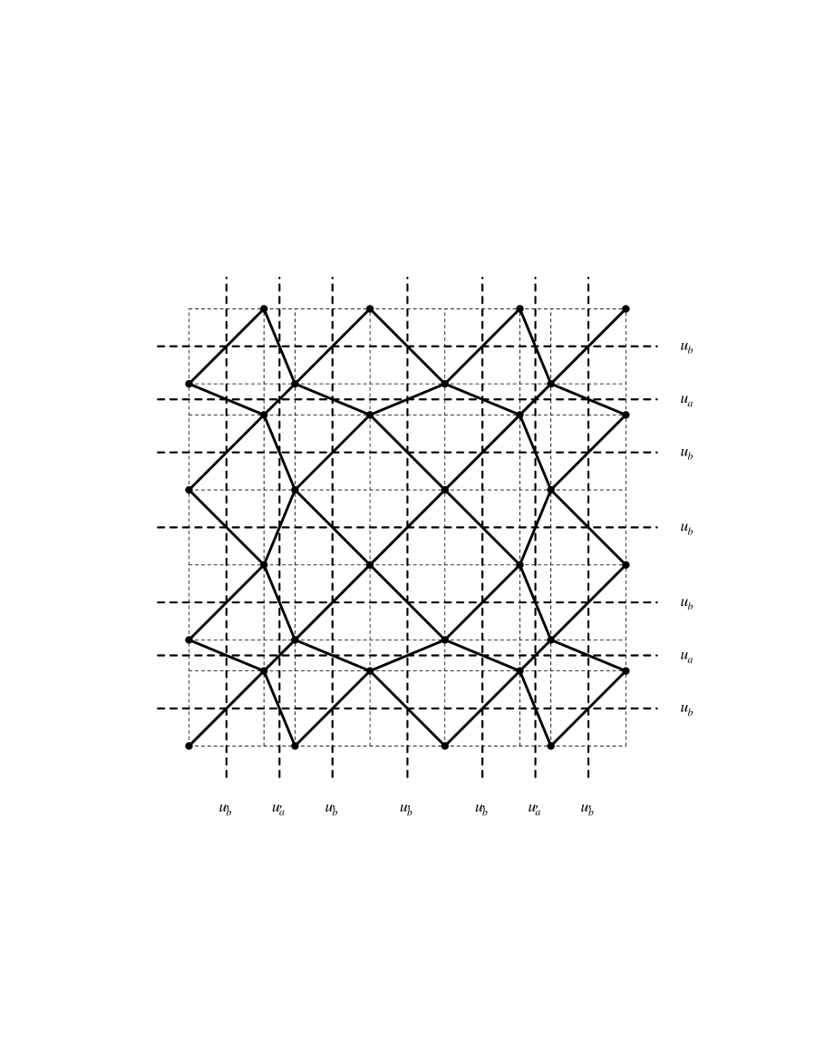
Figure 6: The tiling with rapidity lines and underlying grid

Fig. 6 shows a small section of the Labyrinth tiling with the underlying grid (light) and the rapidity lines (dashed) with the associated parameters. Here, the rapidity lines are constructed parallel to the underlying grid in such way that they divide the edges of the underlying grid into two equal halves. Note that this gives a one-to-one correspondence between the intersections of two rapidity lines and the bonds of the tiling on which the intersection occurs. The checkerboard structure is apparent as the vertices of the Labyrinth lie in rectangles which constitute one of the two sublattices of the rectangular grid formed by the rapidity lines.

It is not possible to give a full account of the actual solution in what follows. Instead, with special focus on the Labyrinth, we summarize the key points of the approach of Ref. [37] which the interested reader should have at hand for cross-reference. Though we can simplify several of the conditions (and actually give the results without derivation) we still depend on the explicit parametrization by elliptic functions which we will now outline.

4.1 Elliptic parametrization and duality

One can explicitly obtain parametrizations of the couplings in the integrable case for three different regimes [37], namely

$$\sinh(2K_{xy}^{\mbox{}})\;=\;F(\eta-u^{\prime}_{x}+u_{y}^{\mbox{}})\;,\hskip 28.45274pt\sinh(2L_{xy}^{\mbox{}})\;=\;F(u^{\prime}_{x}-u_{y}^{\mbox{}})$$ (4.1)

where $F(u)$ is a quotient of Jacobi’s elliptic functions sn($u$), cn($u$), and dn($u$) and where $\eta$ is determined by their half-period magnitudes $K$ and $K^{\prime}$, see Table 1. The rapidities $u_{x}^{\mbox{}}$ and $u^{\prime}_{x}$ ($x\in\{a,b\}$) are a priori arbitrary complex numbers, but in order to obtain real (positive) coupling constants they have to be chosen appropriately, see Ref. [37] for details. In Table 1, we also define several quantities which will be used in what follows. Here, $k$ and $k^{\prime}$ denote the elliptic modulus and conjugate modulus, respectively, and $\Theta(u)$ and $\Theta_{1}(u)$ are the usual Jacobian theta functions [48].

Table 1:   Parametrization in terms of elliptic functions
regime I criticality regime II regime III $\Omega$ $\frac{1}{k^{\prime}}$ $1$ $k^{\prime}$ $\frac{ik^{\prime}}{k}$ $\eta$ $K$ $\frac{\pi}{2}$ $K$ $K-iK^{\prime}$ $F(u)$ $\frac{\mbox{sn($u$)}}{\mbox{cn($u$)}}$ $\tan(u)$ $k^{\prime}\frac{\mbox{sn($u$)}}{\mbox{cn($u$)}}$ $ik^{\prime}\frac{\mbox{sn($u$)}}{\mbox{cn($u$)}}$ $r(u)$ $\frac{\mbox{dn($u$)}}{\mbox{sn($u$)}\mbox{cn($u$)}}$ $\frac{2}{\sin(2u)}$ $\frac{\mbox{dn($u$)}}{\mbox{sn($u$)}\mbox{cn($u$)}}$ $\frac{\mbox{cn($u$)}}{\mbox{sn($u$)}\mbox{dn($u$)}}$ $q(u)$ $\frac{K^{\prime}}{\pi}\frac{\Theta_{1}^{\prime}(u)}{\Theta_{1}(u)}$ $0$ $\frac{K^{\prime}}{\pi}\frac{\Theta^{\prime}(u)}{\Theta(u)}$ $\frac{K^{\prime}}{\pi}\frac{\Theta^{\prime}(u)}{\Theta(u)}$ $c$ $\frac{k^{2}K^{\prime}}{\pi}$ $0$ $-\frac{k^{2}K^{\prime}}{\pi}$ $-\frac{K^{\prime}}{\pi}$

In all regimes, we require the elliptic moduli $k$, $k^{\prime}$ ($k^{\prime}=\sqrt{1-k^{2}}$) to satisfy the inequality $0\leq k,k^{\prime}\leq 1$. Hence, the regimes are characterized by the values of $\Omega$ (which plays the role of a “temperature-like” variable) given in Table 1 as follows: on has $\Omega^{2}>1$, $0<\Omega^{2}<1$ and $\Omega^{2}<0$ for regimes I, II and III, respectively. The critical surface ($\Omega^{2}=1$) separates the “low-temperature” regime I from the disordered “high-temperature” regimes II and III. At all other values of $\Omega$, the partition function turns out to be analytic. We have listed regime III for the sake of completeness because it might become interesting in the context of Lee-Yang zeros in the complex temperature plane.

In the present context, we are mainly interested in regimes I and II as these lead to positive real couplings for the Ising model. In particular, this is the case if one chooses real rapidity differences $u^{\prime}_{x}-u_{y}^{\mbox{}}$ within the range $0<u^{\prime}_{x}-u_{y}^{\mbox{}}<\eta$. Obviously, these two regimes are also related by duality (which inverts $\Omega^{2}$) since the dual couplings (defined by Eqs. (3.22) and (3.23)) are obtained from

$$\sinh(2K_{xy}^{\ast})\;=\;\Omega^{-1}\,F(\eta-u^{\prime}_{x}+u_{y}^{\mbox{}})\;,\hskip 28.45274pt\sinh(2L_{xy}^{\ast})\;=\;\Omega^{-1}\,F(u^{\prime}_{x}-u_{y}^{\mbox{}})\;.$$ (4.2)

Note that in the parametrization given in Table 1 the critical case corresponds to the limits $k\rightarrow 0$, $k^{\prime}\rightarrow 1$, $K\rightarrow\pi/2$, $K^{\prime}\rightarrow\infty$, and $q\rightarrow 0$ where $q=\exp(-\pi K^{\prime}/K)$ is the elliptic nome.

The above parametrization defines a subspace of couplings for which the Ising model is “$Z$-invariant”. The main ingredient in the derivation is, of course, the star-triangle relation [3, 37]. Although we do not want to go into details of the calculation, we still feel that a few words should be spent on the actual conditions on the couplings which are solved by the parametrization (4.1).

The restrictions imposed by the condition of integrability can be conveniently summarized as follows. To this end, it is convenient to introduce another involution $\;\widehat{.}\;$,

$$\widehat{.}\;:\hskip 28.45274pt\left(\begin{array}[]{c}K_{xy}\\ L_{xy}\end{array}\right)\longmapsto\left(\begin{array}[]{c}\widehat{K}_{xy}\\ \mbox{$\!\widehat{\,L\,}\!$}_{xy}\end{array}\right)$$ (4.3)

where $\widehat{K}_{xy}$ and $\mbox{$\!\widehat{\,L\,}\!$}_{xy}$ are implicitly given by

$$\sinh(2\widehat{K}_{xy})\,\sinh(2K_{xy})\;=\;1\;,\hskip 28.45274pt\sinh(2\mbox{$\!\widehat{\,L\,}\!$}_{xy})\,\sinh(2L_{xy})\;=\;1\;.$$ (4.4)

This involution, together with the duality transformation $\;\ast\;$, generates the Abelian group $\mbox{\sf Z\mbox{}Z}_{2}\!\oplus\!\mbox{\sf Z\mbox{}Z}_{2}$ (Klein’s 4-group) which acts on the 8D coupling space $\mbox{\mbox{\hskip 1.00006pt}\rule{0.39993pt}{6.88889pt}\mbox{}{\sf R}}_{+}^{8}$. (Note that $\;\widehat{.}\;$ and $\;\ast\;$ coincided in Sec. 3.4 which was the reason for the “poor” self-duality condition). In the present context, integrability means that the equation

$$\Omega^{2}\;\;=\;\;\prod_{j=1}^{4}\frac{\sinh(2M_{j})\cosh(\widehat{M}_{1}+\widehat{M}_{2}+\widehat{M}_{3}+\widehat{M}_{4}-2\widehat{M}_{j})}{\sinh(2\widehat{M}_{j})\cosh(M_{1}+M_{2}+M_{3}+M_{4}-2M_{j})}$$ (4.5)

has to be satisfied for all vertices, where $M_{j}$ ($j=1,\ldots,4$) denote the couplings on the four surrounding edges of the vertex. In the Labyrinth, we have nine different vertices (counting orientations), cf. Fig. 4, which yield five different equations (due to symmetries). Note that the value of $\Omega$ is the same for all vertices, hence one equation can be regarded as the definition of $\Omega$ and the remaining four result in relations between the couplings. Using the notation of Eq. (3.24), four of the five conditions can actually be simplified to

$$S_{aa}\;=\;S_{ab}\;=\;S_{ba}\;=\;S_{bb}\;=\;\Omega\\$$ (4.6)

which is also apparent in the parametrization given in Table 1 as the function $F$ satisfies

$$F(u)\>F(\eta-u)\;\;=\;\;\Omega$$ (4.7)

in all three regimes.

The one additional equation stems from the vertex which involves one long, one short and two medium length bonds, see Fig. 4. The equivalence of the equations obtained from the four different orientations follows from Eq. (4.6).

Note also that Eq. (4.5) is automatically satisfied for vertex configurations obtained by including words with sequences $\ldots aa\ldots$ which do not occur in the silver mean chain (2.1). This means that the same conditions arise if one considers Ising models on tilings which are defined by different two-letter substitution rules in an analogous way. If one wants to consider models which involve only the four conditions of Eq. (4.6), one is forced to use periodic sequences of just one letter in one direction as this is the only way to avoid the vertex which yields the additional equation.

The conditions (4.5) drastically restrict the possible couplings for the integrable cases. In the “isotropic” case $K_{aa}=L_{aa}=K_{s}$, $K_{ab}=L_{ab}=K_{ba}=L_{ba}=K_{m}$, $K_{bb}=L_{bb}=K_{\ell}$ considered in Sec. 3, the solvable subspace reduces to the isotropic Ising model on the square lattice, since from Eq. (4.6) one obtains $\sinh(2K_{s})=\sinh(2K_{m})=\sinh(2K_{\ell})=\Omega^{1/2}$.

Of course, Eqs. (4.5) and (4.6) are entirely consistent with the results of Sec. 3 as the intersection of the solvable subspace with the self-dual surface (3.26) is just the critical solvable case with $\Omega=1$. One should also realize that it is the additional equation with respect to Eq. (4.6) that actually restricts the solvable critical manifold to a subspace of the self-dual manifold in our case. If one considers models where this equation is absent (which means that one uses a periodic sequence $aaa...$ or $bbb...$ in one direction of the grid on which the tiling is built), the two spaces coincide. It would be interesting to see explicitly how the extra condition in the generic case affects the critical behaviour of the system.

4.2 Partition function and magnetization

Provided that $\Omega$ and all couplings are real and positive, we can follow the techniques outlined in [18, 37, 19, 20] to calculate the partition function in the thermodynamic limit. Here, the result (normalized per site) reads

$$Z\;\;:=\;\;\lim_{n\rightarrow\infty}Z_{n}^{1/N_{n}}\;\;=\;\;{(4\Omega)}^{1/4}\>\exp\left(\frac{1}{2}\mu_{s}\xi_{aa}+\frac{1}{4}\mu_{m}(\xi_{ab}+\xi_{ba})+\frac{1}{2}\mu_{\ell}\xi_{bb}\right)$$ (4.8)

where

$$\xi_{xy}\;\;=\;\;\phi(u^{\prime}_{x}-u_{y}^{\mbox{}})\;+\;\phi(\eta-u^{\prime}_{x}+u_{y}^{\mbox{}})$$ (4.9)

and (cf. Table 1)

$$\phi(u)\;\;=\;\;\frac{1}{2}\,c\,u\;+\;\int_{0}^{u}\,\left(\frac{x}{2K}+q(x)\right)\,r(x)\,dx\;\;.$$ (4.10)

The local spontaneous magnetization $\langle\sigma\rangle$ is given by [37]

$$\langle\sigma\rangle\;\;=\;\;\left\{\begin{array}[]{l@{\hspace*{8mm}}l}{(1-\Omega^{-2})}^{1/8}\hfil\hskip 22.76219pt&\mbox{if $\Omega^{2}>1$}\\ 0\hfil\hskip 22.76219pt&\mbox{if $\Omega^{2}\leq 1$}\end{array}\right.$$ (4.11)

for any single Ising spin of the lattice – wherefore we suppressed the site index in (4.11). One can also easily find expressions for the correlations of two Ising spins that belong to the same plaquette of the Labyrinth tiling [37]. These, of course, depend on the particular couplings along the edges of that plaquette.

The above feature is certainly somewhat surprising as one would expect the one-point function to depend on the local neighbourhood. That this is not the case for the magnetization is clearly due to the conditions (4.6) on the couplings. It is to be expected that one would, for instance, observe a smaller magnetization at the vertices which are surrounded by long bonds only if one chooses $K_{bb}$ and $L_{bb}$ to be small simultaneously (compared to the other couplings) which necessarily violates Eq. (4.6). In this sense, the integrable subspace is possibly not representative and we presently cannot exclude the possibility of more than one phase transition in the general case where the corresponding order parameters would be the magnetization of certain subsets of the Labyrinth vertices.

5 Concluding remarks

A zero-field Ising model on the Labyrinth tiling has been investigated. We used duality arguments to obtain information about the location of critical points and determined the self-dual couplings. Also, the subclass of exactly solvable models was considered in detail, following closely the discussion of the checkerboard Ising model in Ref. [37]. In this case, the self-dual couplings also define the critical surface, the transition being of the Onsager type as in the periodic model.

The special model investigated here is, of course, just an example. It can be generalized to tilings obtained by an analogous procedure from arbitrary two-letter substitution rules, provided one uses the correct periodic approximants. In this way, one can study Ising systems where the fluctuations of the underlying tiling behave in different ways. This is of interest because it has recently been shown in several closely related examples that these fluctuations actually determine the critical behaviour of the Ising model, see e.g. [16, 14, 15, 17].

Of course, the investigation of the solvable cases can only be the first step in the investigation of the critical properties of Ising models on aperiodic tilings, and we hope to report on further results soon. The exactly solvable $Z$-invariant case is arguably too restrictive to be assumed representative as it, for instance, forces the magnetization to be independent of the location, which will certainly not be the case for some arbitrarily chosen couplings.

Finally, one can extend the analysis to other systems like the more general eight-vertex model in the spirit of [18, 19, 20]. Here, it is now relatively clear what happens in the solvable cases which are, by no means, restricted to de Bruijn grids, cf. [21]. However, any progress beyond local solvability would help understanding the hierarchy of critical phenomena between periodic and random.

Figure 1: The Labyrinth with underlying grid and boundary conditions

Figure 2: The Labyrinth and its dual

Figure 3: The tiling and its inflation

Figure 4: The tiles and their dual vertex configurations

Figure 5: Assignment of couplings $K_{xy}$ and $L_{xy}$ ($xy\in\{aa,ab,ba,bb\}$)

References

- [1]
- [2] J. L. Cardy, Conformal Invariance, in: Phase Transitions and Critical Phenomena, vol. 11, eds. C. Domb und J. L. Lebowitz, Academic Press, London (1987).
- [3] R. J. Baxter, Exactly Solved Models in Statistical Mechanics, Academic Press, London (1982).
- [4] V. Bazhanov, Trigonometric Solutions of Triangle Equations and Classical Lie Algebras, Phys. Lett. B159 (1985) 321; M. Jimbo, Quantum Matrix for the Generalized Toda System, Commun. Math. Phys. 102 (1986) 537; A. Kuniba, Quantum matrix for G2 and a solvable 175-vertex model, J. Phys. A23 (1990) 1349; Z.-Q. Ma, The spectrum-dependent solutions to the Yang-Baxter equation for quantum E6 and E7, J. Phys. A23 (1990) 5513; J. D. Kim, I. G. Koh and Z.-Q. Ma, Quantum matrix for and groups, J. Math. Phys. 32 (1991) 845; H. J. Chung and I. G. Koh, Solutions to the quantum Yang-Baxter equation for the exceptional Lie algebras with a spectral parameter, J. Math. Phys. 32 (1991) 2406.
- [5] G. E. Andrews, R. J. Baxter and P. J. Forrester, Eight-Vertex SOS Model and Generalized Rogers-Ramanujan-Type Identities J. Stat. Phys. 35 (1984) 193;
- [6] G. von Gehlen and V. Rittenberg, -symmetric quantum chains with an infinite set of conserved charges and zero modes, Nucl. Phys. B257 (1985) 351.
- [7] R. J. Baxter, The superintegrable chiral Potts model, Phys. Lett. A133 (1988) 185.
- [8] R. Kedem and B. M. McCoy, Quasi-Particles in the Chiral Potts Model, Int. J. Mod. Phys. B8 (1994) 3601
- [9] V. V. Bazhanov and R. J. Baxter, Star-Triangle Relation for a Three-Dimensional Model, J. Stat. Phys. 71 (1993) 839. V. Pasquier, Two-dimensional critical systems labelled by Dynkin diagrams, Nucl. Phys. B285 (1987) 162; E. Date, M. Jimbo, A. Kuniba, T. Miwa and M. Okado, Exactly solvable SOS models: Local height probabilities and theta function identities, Nucl. Phys. B290 (1987) 231; E. Date, M. Jimbo, A. Kuniba, T. Miwa and M. Okado, Exactly solvable SOS models II: Proof of the star-triangle relation and combinatorical identities, Adv. Stud. Pure Math. 16 (1988) 17; M. Jimbo, A. Kuniba, T. Miwa and M. Okado, The Face Models, Commun. Math. Phys. 119 (1988) 543; M. Jimbo, T. Miwa, and M. Okado, Solvable Lattice Models Related to the Vector Representation of Classical Simple Lie Algebras, Commun. Math. Phys. 116 (1988) 507; A. Kuniba, Exact solution of solid-on-solid models for twisted affine Lie algebras and , Nucl. Phys. B355 (1991) 801; A. Kuniba and J. Suzuki, Exactly solvable solid-on-solid models, Phys. Lett. A160 (1991) 216.
- [10] S. O. Warnaar, B. Nienhuis and K. A. Seaton, New Construction of Solvable Lattice Models Including an Ising Model in a Field, Phys. Rev. Lett. 69 (1992) 710; S. O. Warnaar and B. Nienhuis, Solvable lattice models labelled by Dynkin diagrams, J. Phys. A26 (1993) 2301; S. O. Warnaar, B. Nienhuis and K. A. Seaton, A Critical Ising Model in a Magnetic Field, Int. J. Mod. Phys. B7 (1993) 3727; S. O. Warnaar, P. A. Pearce, K. A. Seaton and B. Nienhuis, Order Parameters of the Dilute A Models, J. Stat. Phys. 74 (1994) 469; S. O. Warnaar, Algebraic construction of higher rank dilute A models, Nucl. Phys. B435 (1995) 463.
- [11] M. Baake, U. Grimm and C. Pisani, Partition Function Zeros for Aperiodic Systems, J. Stat. Phys. 78 (1995) 285.
- [12] V. G. Benza, Quantum Ising Quasi-Crystal, Europhys. Lett. 8 (1989) 321.
- [13] Z. Lin and R. Tao, Phase transition in aperiodic quantum Ising chains constructed with arbitrary substitution rules, Phys. Rev. B46 (1992) 10808.
- [14] J. M. Luck, Critical Behavior of the Aperiodic Quantum Ising Chain in a Transverse Magnetic Field, J. Stat. Phys. 72 (1993) 417.
- [15] U. Grimm and M. Baake, Non-Periodic Ising Quantum Chains and Conformal Invariance, J. Stat. Phys. 74 (1994) 1233.
- [16] C. A. Tracy, Universality classes of some aperiodic Ising models, J. Phys. A21 (1988) L603.
- [17] F. Iglói, Critical behaviour in aperiodic systems, J. Phys. A26 (1993) L703.
- [18] R. J. Baxter, Solvable eight-vertex model on an arbitrary planar lattice, Phil. Trans. R. Soc. Lond. 289 (1978) 315.
- [19] V. E. Korepin, Eight-vertex model of the quasicrystal, Phys. Lett. A118 (1986) 285; V. E. Korepin, Exactly solvable spin models in quasicrystals, Sov. Phys. JETP 65 (1986) 614; V. E. Korepin, Completely integrable models in quasicrystals, Commun. Math. Phys. 110 (1987) 157.
- [20] T. C. Choy, Ising models on two-dimensional quasi-crystals: some exact results, Int. J. Mod. Phys. B2 (1988) 49.
- [21] N. G. de Bruijn, Algebraic theory of Penrose’s non-periodic tilings of the plane, part I, Math. Proc. A84 (1981) 39-52, and part II, Math. Proc. A84 (1981) 53-66.
- [22] C. Godrèche, J.-M. Luck and H. Orland, Magnetic Phase Structure on the Penrose Lattice, J. Stat. Phys. 45 (1986) 777.
- [23] H. Aoyama and T. Odagaki, Eight-Parameter Renormalization Group for Penrose Lattices, J. Stat. Phys. 48 (1987) 503.
- [24] A. Doroba and K. Sokalski, The Ising Model on the Two-Dimensional Quasiperiodic Lattice, Physica stat. sol. B152 (1989) 275.
- [25] S. M. Bhattacharjee, J.-S. Ho and J. A. Y. Johnson, Translational invariance in critical phenomena: Ising model on a quasi-lattice, J. Phys. A20 (1987) 4439.
- [26] G. Amarenda, G. Ananthakrishna and G. Athithan, Critical Behavior of the Ising Model on a Two-Dimensional Penrose Lattice, Europhys. Lett. 5 (1988) 181.
- [27] Y. Okabe and K. Niizeki, Monte Carlo Simulation of the Ising Model on the Penrose Lattice, J. Phys. Soc. Japan 57 (1988) 16.
- [28] Y. Okabe and K. Niizeki, Duality in the Ising model on quasicrystals, J. Phys. Soc. Japan 57 (1988) 1536; Y. Okabe and K. Niizeki, Phase transition of the Ising model on the two-dimensional quasicrystals, J. Phys. Colloq. (France) 49 (1988) 1387.
- [29] W. G. Wilson and C. A. Vause, Evidence for universality of the Potts model on the two-dimensional Penrose lattice, Phys. Lett. A126 (1988) 471.
- [30] R. Abe and T. Dotera, High-Temperature Expansion for the Ising Model on the Penrose Lattice, J. Phys. Soc. Japan 58 (1989) 3219; T. Dotera and R. Abe, High-Temperature Expansion for the Ising Model on the Dual Penrose Lattice, J. Phys. Soc. Japan 59 (1990) 2064.
- [31] E. S. Sørensen, M. V. Jarić and M. Ronchetti, Ising model on Penrose lattices: boundary conditions, Phys. Rev. B44 (1991) 9271.
- [32] C. Sire, R. Mosseri and J.-F. Sadoc, Geometric study of a 2D tiling related to the octagonal quasiperiodic tiling, J. Phys. France 50 (1989) 3463.
- [33] R. Peierls, On Ising’s model of ferromagnetism, Proc. Cambridge Phil. Soc. 32 (1936) 477.
- [34] R. B. Griffiths, Rigorous Results and Theorems, in: Phase Transitions and Critical Phenomena, vol. 1, eds. C. Domb and M. S. Green, Academic Press, London (1972).
- [35] R. S. Ellis, Entropy, Large Deviations, and Statistical Mechanics, Springer, New York (1985).
- [36] D. W. Wood, A self dual relation for a three dimensional assembly, J. Phys. C5 (1972) L181; P. A. Pearce and R. J. Baxter, Duality of the three-dimensional Ising model with quartet interactions, Phys. Rev. B24 (1981) 5295; R. Liebmann, Monte Carlo Study of the Quartet Ising Model Consistent with Selfduality, Z. Phys. B45 (1982) 243.
- [37] R. J. Baxter Free-fermion, checkerboard and -invariant lattice models in statistical mechanics, Proc. R. Soc. Lond. A404 (1986) 1.
- [38] N. V. Antonov and V. E. Korepin, Critical properties of completely integrable spin models in quasicrystals, Theor. Math. Phys. 77 (1988) 1282.
- [39] A. Doroba, Equivalence of the Ising model on the 2-D Penrose and 2-D regular lattices, Acta Phys. Pol. A76 (1989) 949.
- [40] C. Sire, Electronic Spectrum of a 2D Quasi-Crystal Related to the Octagonal Quasi-Periodic Tiling, Europhys. Lett. 10 (1989) 483.
- [41] M. Baake, U. Grimm and D. Joseph, Trace maps, invariants, and some of their applications, Int. J. Mod. Phys. B7 (1993) 1527.
- [42] A. Katz, On the distinction between quasicrystals and modulated crystals, in: Quasicrystals, eds. M. V. Jarić and S. Lundqvist, World Scientific, Singapore (1990), p. 200.
- [43] H. A. Kramers and G. H. Wannier, Statistics of the Two-Dimensional Ferromagnet. Part I, Phys. Rev. 60 (1941) 252.
- [44] M. Duneau, F. Dunlop and C. Oguey, Ground states of frustrated Ising quasicrystals, J. Phys. A26 (1993) 2791.
- [45] J. M. Luck, Frustration effects in qusicrystals: an exactly soluble example in one dimension, J. Phys. A20 (1987) 1259.
- [46] C. Sire, Ising chain in a quasiperiodic magnetic field, Int. J. Mod. Phys. B7 (1993) 1551.
- [47] J. Oitmaa, M. Aydin, and M. J. Johnson, Antiferromagnetic Ising model on the Penrose lattice, J. Phys. A23 (1990) 4537.
- [48] I. S. Gradshteyn and I. M. Ryzhik, Tables of Integrals, Series and Products, 5th ed., Academic Press, London (1993).
- [49]