Discrete time Lagrangian mechanics on Lie groups,
with an application to the Lagrange top

Abstract

We develop the theory of discrete time Lagrangian mechanics on Lie groups, originated in the work of Veselov and Moser, and the theory of Lagrangian reduction in the discrete time setting. The results thus obtained are applied to the investigation of an integrable time discretization of a famous integrable system of classical mechanics, – the Lagrange top. We recall the derivation of the Euler–Poinsot equations of motion both in the frame moving with the body and in the rest frame (the latter ones being less widely known). We find a discrete time Lagrange function turning into the known continuous time Lagrangian in the continuous limit, and elaborate both descriptions of the resulting discrete time system, namely in the body frame and in the rest frame. This system naturally inherits Poisson properties of the continuous time system, the integrals of motion being deformed. The discrete time Lax representations are also found. Kirchhoff’s kinetic analogy between elastic curves and motions of the Lagrange top is also generalised to the discrete context.

1 Introduction

This paper is devoted to the time discretization of a famous integrable system of classical mechanics – the Lagrange top. This is a special case of rotation of a rigid body around a fixed point in a homogenious gravitational field, characterized by the following conditions: the rigid body is rotationally symmetric, i.e. two of its three principal moments of inertia coincide, and the fixed point lies on the axis of rotational symmetry. We present a discretization preserving the integrability property, and discuss its rich mechanical and geometrical structure. Notice that until recently [B] only the integrable Euler case of the rigid body motion was discretized preserving integrability [V], [MV], [BLS]. Consult also [AL], [H], [DJM], [QNCV] for some fundamental early papers on the subject of integrable discretizations, and [BP], [S] for reviews of this topic reflecting the viewpoints of the present authors and containing extensive bibliography.

We found the standard presentation of the Lagrange top in mechanical textbooks insufficient in several respects, and therefore chose to write this paper in a pedagogical manner, giving a systematic account of the new results along with the well known ones represented in a form suitable for our present purposes. The paper is organized as follows.

The introduction recalls the classical Euler–Poinsot equations for the motion of the spinning top in the frame moving with the body. Further, we give less known Euler–Poinsot equations describing the Lagrange top in the rest frame (they cannot be directly generalized to a general top case). We finish the introduction by announcing a beautiful time discretization of the latter equations.

In order to derive this discretization systematically, we need some formalism of discrete time Lagrangian mechanics on Lie groups. The discrete time Lagrangian mechanics were introduced by Veselov [V], [MV], see also [WM], but the case of Lie groups have certain specific features which, in our opinion, were not worked out sufficiently. In particular, there lacks a systematic account of the discrete time version of the Lagrangian reduction (which is fairly well understood in the continuous time setting, cf. [MS], [HMR]). Also, we think that some technical details in [V], [MV], [WM] could be amended: in working with variational equations these authors systematically use Lagrange multipliers instead of introducing proper notions such as Lie derivatives (specific for Lie groups as opposed to general manifolds). Therefore we give a detailed exposition of the discrete time Lagrangian mechanics on Lie groups in Sect. 3. In order to underline an absolute parallelism of its structure with that of the continuous time Lagrangian mechanics, we included in Sect. 2 also a presentation of (a fragment of) the latter, which is, of course, by no means original.

Sect. 4 is devoted to a Lagrangian derivation of equations of motion of the Lagrange top, both in the rest and in the body frames. Finally, in Sect. 5 we do the same work for a discrete time Lagrange top.

It has to be mentioned that the actual motivation for the present development came from differential geometry, more precisely, from the theory of elastic curves. A brief account of the relations between spinning tops and elastic curves is given in Sect. 6.

We also give three appendices. Appendix A is for fixing the notations of Lie group theory. In the Appendix B we collect the main results of Sect. 2, 3 in the form of an easy–to–use table. Finally, Appendix C contains some conventions and simple technical results on a specific Lie group we work with, namely on $SU(2)$. It should be remarked here that our experience with various integrable discretizations convinced us that working with this group has many advantages when compared to the group $SO(3)$, more traditional in this context.

A standard form of equations of motion describing rotation of a rigid body around a fixed point in a homogeneous gravity field is the following:

$$\left\{\begin{array}[]{l}\dot{M}=M\times\Omega(M)+P\times A\\ \\ \dot{P}=P\times\Omega(M)\end{array}\right.$$ (1.1)

Here $M=(M_{1},M_{2},M_{3})^{T}\in{{R}}^{3}$ is the vector of kinetic momentum of the body, expressed in the so called body frame. This frame is firmly attached to the body, its origin is in the body’s fixed point, and its axes coincide with the principal inertia axes of the body. The inertia tensor of the body in this frame is diagonal:

$$J=\left(\begin{array}[]{ccc}J_{1}&0&0\\ 0&J_{2}&0\\ 0&0&J_{3}\end{array}\right)\;.$$ (1.2)

For the vector $\Omega=\Omega(M)$ of the angular velocity we have:

$$\Omega=\Omega(M)=J^{-1}M=(J_{1}^{-1}M_{1},J_{2}^{-1}M_{2},J_{3}^{-1}M_{3})^{T}\in{{R}}^{3}\;.$$ (1.3)

The vector $P=(P_{1},P_{2},P_{3})^{T}\in{{R}}^{3}$ is the unit vector along the gravity field, with respect to the body frame. Finally, $A=(A_{1},A_{2},A_{3})^{T}\in{{R}}^{3}$ is the vector pointing from the fixed point to the center of mass of the body. It is a constant vector in the body frame.

It is well known that the system (1.1) is Hamiltonian with respect to the Lie–Poisson bracket of the Lie algebra $e(3)$ of the Lie group $E(3)$ of euclidean motions of ${{R}}^{3}$, i.e. with respect to the Poisson bracket

$$\{M_{i},M_{j}\}=\varepsilon_{ijk}M_{k}\;,\qquad\{M_{i},P_{j}\}=\varepsilon_{ijk}P_{k}\;,\qquad\{P_{i},P_{j}\}=0\;,$$ (1.4)

where $\varepsilon_{ijk}$ is the sign of the permutation $(ijk)$ of $(123)$. The Hamiltonian equations of motion for an arbitrary Hamilton function $H=H(M,P)$ in the bracket (1.4) read:

$$\left\{\begin{array}[]{l}\dot{M}=M\times\nabla_{M}H+P\times\nabla_{P}H\\ \\ \dot{P}=P\times\nabla_{M}H\end{array}\right.$$ (1.5)

which coincides with (1.1) if

$$H(M,P)=\frac{1}{2}\langle M,\Omega(M)\rangle+\langle P,A\rangle\;.$$ (1.6)

(Here $\langle\cdot,\cdot\rangle$ stands for the standard euclidean scalar product in ${{R}}^{3}$). The Poisson bracket (1.4) has two Casimir functions,

$$C=\langle M,P\rangle\qquad{\rm and}\qquad\langle P,P\rangle\;,$$ (1.7)

which are therefore integrals of motion for (1.1) in involution with $H(M,P)$ (and with any other function on the phase space).

The Lagrange case of the rigid body motion (the Lagrange top, for brevity), is characterized by the following data: $J_{1}=J_{2}$, which means that the body is rotationally symmetric with respect to the third coordinate axis), and $A_{1}=A_{2}=0$, which means that the fixed point lies on the symmetry axis. Choosing units properly, we may assume that

$$J_{1}=J_{2}=1\;,\qquad J_{3}=\alpha\;,\qquad A=(0,0,1)^{T}\;.$$ (1.8)

The system (1.1) has in this case an additional integral of motion,

$$M_{3}=\langle M,A\rangle\;,$$ (1.9)

which is also in involution with $H(M,P)$, and assures therefore the complete integrability of the flow (1.1). For an actual integration of this flow in terms of elliptic functions see, e.g., [G], [KS], and for a more modern account [RM], [Au], [CB].

Remarkable as it is, this result is, however, somewhat unsatisfying from the practical point of view. Indeed, one is usually interested in describing the motion of the top in the rest frame, which does not move in the physical space. It is less known that for the Lagrange top the corresponding equations of motion are also very nice and, actually, even somewhat simpler than (1.1):

$$\left\{\begin{array}[]{l}\dot{m}=p\times a\\ \\ \dot{a}=m\times a\end{array}\right.$$ (1.10)

Here $m=(m_{1},m_{2},m_{3})^{T}\in{{R}}^{3}$ is the vector of kinetic momentum of the body, expressed in the rest frame, $p$ is the unit vector along the gravity field, also expressed in the rest frame, so that it becomes constant:

$$p=(0,0,1)^{T}\;,$$ (1.11)

and $a=(a_{1},a_{2},a_{3})^{T}\in{{R}}^{3}$ is the vector pointing from the fixed point to the center of mass, expressed in the rest frame. An exterior observer is mainly interested in the motion of the symmetry axis of the top, which is described by the vector $a$.

The system (1.10) has several remarkable features. First of all, it does not depend explicitly on the anisotropy parameter $\alpha$ of the inertia tensor. Second, it is Hamiltonian with respect to the Lie–Poisson bracket of $e(3)$:

$$\{m_{i},m_{j}\}=-\varepsilon_{ijk}m_{k}\;,\qquad\{m_{i},a_{j}\}=-\varepsilon_{ijk}a_{k}\;,\qquad\{a_{i},a_{j}\}=0\;.$$ (1.12)

For an arbitrary Hamilton function $H(m,a)$, the Hamiltonian equations of motion in this bracket read:

$$\left\{\begin{array}[]{l}\dot{m}=\nabla_{m}H\times m+\nabla_{a}H\times a\\ \\ \dot{a}=\nabla_{m}H\times a\end{array}\right.$$ (1.13)

These equations coincide with (1.10), if

$$H_{0}(m,a)=\frac{1}{2}\langle m,m\rangle+\langle p,a\rangle\;.$$ (1.14)

Of course, the functions

$$c=\langle m,a\rangle\qquad{\rm and}\qquad\langle a,a\rangle\;,$$ (1.15)

are Casimirs of the bracket (1.12), and therefore are integrals of motion for (1.10) in involution with $H_{0}(m,a)$ (and with any other function on the phase space). An additional integral of motion in involution with $H_{0}(m,a)$, assuring the complete integrability of the system (1.10), is:

$$m_{3}=\langle m,p\rangle\;.$$ (1.16)

In the main text we give a Lagrangian derivation of equations of motion (1.1) and (1.10) and an explanation of their Hamiltonian nature and integrability. Then we present a discrete Lagrangian function generating two maps approximating (1.1) and (1.10), respectively. Most beautiful is the discretization of (1.10):

$$\left\{\begin{array}[]{l}m_{k+1}-m_{k}=\varepsilon\,p\times a_{k}\;,\\ \\ a_{k+1}-a_{k}=\displaystyle\frac{\varepsilon}{2}\,m_{k+1}\times(a_{k}+a_{k+1})\;.\end{array}\right.$$ (1.17)

It is easy to see that the second equation in (1.17) can be uniquely solved for $a_{k+1}$, so that (1.17) defines a map $(m_{k},a_{k})\mapsto(m_{k+1},a_{k+1})$, approximating, for small $\varepsilon$, the time $\varepsilon$ shift along the trajectories of (1.10). This distinguishes the situation from the one in [MV] where Lagrangian equations led to correspondences rather than to maps. We shall demonstrate that the map (1.17) is Poisson with respect to the bracket (1.12), so that the Casimirs (1.15) are integrals of motion. It is also obvious that (1.16) is an integral of motion. Most remarkably, this map has another integral of motion – an analog of the Hamiltonian:

$$H_{\varepsilon}(m,a)=\frac{1}{2}\langle m,m\rangle+\langle a,p\rangle+\frac{\varepsilon}{2}\langle a\times m,p\rangle\;.$$ (1.18)

The function (1.18) is in involution with (1.16), which renders the map (1.17) completely integrable. A similar discretization for the equations of motion in the body frame (1.1) is slightly less elegant.

2 Lagrangian mechanics on $TG$
(continuous time case)

Let ${\bf L}(g,\dot{g})\,:\,TG\mapsto{{R}}$ be a smooth function on the tangent bundle of the Lie group $G$, called the Lagrange function. For an arbitrary function $g(t)\,:\,[t_{0},t_{1}]\mapsto G$ one can consider the action functional

$$S=\int_{t_{0}}^{t_{1}}{\bf L}(g(t),\dot{g}(t))dt\;.$$ (2.1)

A standard argument shows that the functions $g(t)$ yielding extrema of this functional (in the class of variations preserving $g(t_{0})$ and $g(t_{1})$), satisfy with necessity the Euler–Lagrange equations. In local coordinates $\{g^{i}\}$ on $G$ they read:

$$\frac{d}{dt}\left(\frac{\partial{\bf L}}{\partial\dot{g}^{i}}\right)=\frac{\partial{\bf L}}{\partial g^{i}}\;.$$ (2.2)

The action functional $S$ is independent of the choice of local coordinates, and thus the Euler–Lagrange equations are actually coordinate independent as well. For a coordinate–free description in the language of differential geometry, see [A], [MR].

Introducing the quantities

$$\Pi=\nabla_{\dot{g}}{\bf L}\in T_{g}^{*}G\;,$$ (2.3)

one defines the Legendre transformation:

$$(g,\dot{g})\in TG\mapsto(g,\Pi)\in T^{*}G\;.$$ (2.4)

If it is invertible, i.e. if $\dot{g}$ can be expressed through $(g,\Pi)$, then the the Legendre transformation of the Euler–Lagrange equations (2.2) yield a Hamiltonian system on $T^{*}G$ with respect to the standard symplectic structure on $T^{*}G$ and with the Hamilton function

$$H(g,\Pi)=\langle\Pi,\dot{g}\rangle-{\bf L}(g,\dot{g})\;,$$ (2.5)

(where, of course, $\dot{g}$ has to be expressed through $(g,\Pi)$). Finally, we want to mention the Noether construction for deriving the existence of integrals of motion of the Euler–Lagrange equations from the symmetry groups of the Lagrange function. We shall formulate the simplest form of Noether’s theorem, where Lagrangian functions are invariant under the action of one–dimensional groups. Let $\zeta\in{{g}}$ be a fixed element, and consider a one–parameter subgroup

$$G^{(\zeta)}=\{e^{c\zeta}\,:\,c\in{{R}}\}\subset G\;.$$ (2.6)

Proposition 2.1

1. Let the Lagrange function be invariant under the action of $G^{(\zeta)}$ on $TG$ induced by left translations on $G$:

   $${\bf L}(e^{c\zeta}g,L_{e^{c\zeta}*}\dot{g})={\bf L}(g,\dot{g})\;.$$ (2.7)

   Then the following function is an integral of motion of the Euler–Lagrange equations:

   $$\langle R_{g}^{*}(\nabla_{\dot{g}}{\bf L}),\zeta\rangle=\langle R_{g}^{*}\Pi,\zeta\rangle\;.$$ (2.8)

2. Let the Lagrange function be invariant under the action of $G^{(\zeta)}$ on $TG$ induced by right translations on $G$:

   $${\bf L}(ge^{c\zeta},R_{e^{c\zeta}*}\dot{g})={\bf L}(g,\dot{g})\;.$$ (2.9)

   Then the following function is an integral of motion of the Euler–Lagrange equations:

   $$\langle L_{g}^{*}(\nabla_{\dot{g}}{\bf L}),\zeta\rangle=\langle L_{g}^{*}\Pi,\zeta\rangle\;.$$ (2.10)

Proof. Differentiate (2.7) (or (2.9)) with respect to $c$, set $c=0$, and use the Euler–Lagrange equations.  

For a detailed proof of the general version of the Noether theorem see [A], [MR].

In practice, it turns out to be more convenient to work not with the tangent bundle $TG$, but with its trivializations $G\times{{g}}$, which is achieved by translating the vector $\dot{g}\in T_{g}G$ into the group unit via left or right translations.

2.1 Left trivialization

Consider the trivialization map

$$(g,\Omega)\in G\times{{g}}\mapsto(g,\dot{g})\in TG\;,$$ (2.11)

where

$$\dot{g}=L_{g*}\Omega\quad\Leftrightarrow\quad\Omega=L_{g^{-1}*}\dot{g}\;.$$ (2.12)

The trivialization (2.11) of the tangent bundle $TG$ induces the following trivialization of the cotangent bundle $T^{*}G$:

$$(g,M)\in G\times{{g}}^{*}\mapsto(g,\Pi)\in T^{*}G\;,$$ (2.13)

where

$$\Pi=L_{g^{-1}}^{*}M\quad\Leftrightarrow\quad M=L_{g}^{*}\Pi\;.$$ (2.14)

Denote the pull–back of the Lagrange function through

$${\bf L}^{(l)}(g,\Omega)={\bf L}(g,\dot{g})\;,$$ (2.15)

so that

$${\bf L}^{(l)}(g,\Omega)\,:\,G\times{{g}}\mapsto{{R}}\;.$$

We want to find differential equations satisfied by those functions $(g(t),\Omega(t))\,:\,[t_{0},t_{1}]\mapsto G\times{{g}}$ delivering extrema of the action functional

$$S^{(l)}=\int_{t_{0}}^{t_{1}}{\bf L}^{(l)}(g(t),\Omega(t))dt$$

and such that

$$\Omega(t)=L_{g^{-1}(t)*}\dot{g}(t)\;.$$

Admissible variations of $(g(t),\Omega(t))$ are those preserving the latter equality and the values $g(t_{0})$, $g(t_{1})$.

Proposition 2.2

The differential equations for extremals of the functional $S^{(l)}$ read:

$$\left\{\begin{array}[]{l}\dot{M}={\rm ad}^{*}\,\Omega\cdot M+d\,^{\prime}_{\!g}{\bf L}^{(l)}\;,\\ \\ \dot{g}=L_{g*}\Omega\;,\end{array}\right.$$ (2.16)

where

$$M=\nabla_{\Omega}{\bf L}^{(l)}\in{{g}}^{*}\;.$$ (2.17)

If the Legendre transformation

$$(g,\Omega)\in G\times{{g}}\mapsto(g,M)\in G\times{{g}}^{*}$$ (2.18)

is invertible, it turns (2.16) into a Hamiltonian form on $G\times{{g}}^{*}$ with the Hamilton function

$$H(g,M)=\langle M,\Omega\rangle-{\bf L}^{(l)}(g,\Omega)\;,$$ (2.19)

(where, of course, $\Omega$ has to be expressed through $(g,M)$); the underlying invariant Poisson bracket on $G\times{{g}}^{*}$ is the pull–back of the standard symplectic bracket on $T^{*}G$, so that for two arbitrary functions $f_{1,2}(g,M)\,:\,G\times{{g}}^{*}\mapsto{{R}}$ we have:

$$\{f_{1},f_{2}\}=-\langle d\,^{\prime}_{\!g}f_{1},\nabla_{M}f_{2}\rangle+\langle d\,^{\prime}_{\!g}f_{2},\nabla_{M}f_{1}\rangle+\langle M,[\nabla_{M}f_{1},\nabla_{M}f_{2}]\,\rangle\;.$$ (2.20)

Proof. The equations of motion (2.16) may be derived by pulling back the equations (2.2) under the trivialization map (2.11), but it is somewhat simpler to derive them independently. To this end, consider the admissible variations of $(g(t),\Omega(t))$ in the form

$$g(t,\epsilon)=g(t)e^{\epsilon\eta(t)}\;,\quad{\rm where}\quad\eta(t)\,:\,[t_{0},t_{1}]\mapsto{{g}}\;,\quad\eta(t_{0})=\eta(t_{1})=0\;,$$

and

$$\Omega(t,\epsilon) = L_{g^{-1}(t,\epsilon)*}\dot{g}(t,\epsilon)={\rm Ad}\,e^{-\epsilon\eta(t)}\cdot\Omega(t)+\epsilon\dot{\eta}(t)+O(\epsilon^{2})$$

$$= \Omega(t)+\epsilon\Big{(}\dot{\eta}(t)+[\Omega(t),\eta(t)]\Big{)}+O(\epsilon^{2})\;.$$

So, equating the variation of action to zero, we get:

$$0=\left.\frac{dS^{(l)}}{d\epsilon}\right|_{\epsilon=0}=\int_{t_{0}}^{t_{1}}\Big{(}\langle\,d\,^{\prime}_{\!g}{\bf L}^{(l)},\eta\,\rangle+\langle\nabla_{\Omega}{\bf L}^{(l)},\dot{\eta}+{\rm ad}\,\Omega\cdot\eta\,\rangle\Big{)}\,dt\;.$$

Integrating the term with $\dot{\eta}$ by parts and taking into account $\eta(t_{0})=\eta(t_{1})=0$, we come to:

$$\int_{t_{0}}^{t_{1}}\langle\,d\,^{\prime}_{\!g}{\bf L}^{(l)}+{\rm ad}^{*}\,\Omega\cdot\nabla_{\Omega}{\bf L}^{(l)}-\frac{d}{dt}(\nabla_{\Omega}{\bf L}^{(l)}),\eta\,\rangle\,dt=0\;.$$

Due to arbitariness of $\eta(t)$ the following equation holds:

$$\frac{d}{dt}(\nabla_{\Omega}{\bf L}^{(l)})={\rm ad}^{*}\,\Omega\cdot\nabla_{\Omega}{\bf L}^{(l)}+d\,^{\prime}_{\!g}{\bf L}^{(l)}\;.$$

It remains to notice that $M$ defined by (2.14), (2.3), i.e. $M=L_{g}^{*}\nabla_{\dot{g}}{\bf L}$, coincides with (2.17), as it follows from (2.12).  

We now observe, what does Noether’s theorem (more exactly, its version in Proposition 2.1) yield under left trivialization.

Proposition 2.3

1. Let the Lagrange function ${\bf L}^{(l)}(g,\Omega)$ be invariant under the action of $G^{(\zeta)}$ on $G\times{{g}}$ induced by left translations on $G$:

   $${\bf L}^{(l)}(e^{c\zeta}g,\Omega)={\bf L}^{(l)}(g,\Omega)\;.$$ (2.21)

   Then the following function is an integral of motion of the Euler–Lagrange equations:

   $$\langle{\rm Ad}^{*}\,g^{-1}\cdot\nabla_{\Omega}{\bf L}^{(l)},\zeta\rangle=\langle M,{\rm Ad}\,g^{-1}\cdot\zeta\rangle\;.$$ (2.22)

2. Let the Lagrange function ${\bf L}^{(l)}(g,\Omega)$ be invariant under the action of $G^{(\zeta)}$ on $G\times{{g}}$ induced by right translations on $G$:

   $${\bf L}^{(l)}(ge^{c\zeta},{\rm Ad}\,e^{-c\zeta}\cdot\Omega)={\bf L}^{(l)}(g,\Omega)\;.$$ (2.23)

   Then the following function is an integral of motion of the Euler–Lagrange equations:

   $$\langle\nabla_{\Omega}{\bf L}^{(l)},\zeta\rangle=\langle M,\zeta\rangle\;.$$ (2.24)

We finish this subsection by discussing the reduction procedure relevant for later applications. Let us assume that there holds a condition somewhat stronger than (2.21), namely, that the function ${\bf L}^{(l)}$ is left invariant under the action of a subgroup somewhat larger than $G^{(\zeta)}$. Fix an element $\zeta\in{{g}}$, and consider the isotropy subgroup $G^{[\zeta]}$ of $\zeta$ with respect to the adjoint action of $G$, i.e.

$$G^{[\zeta]}=\{h\,:\;{\rm Ad}\,h\cdot\zeta=\zeta\}\subset G\;.$$ (2.25)

Obviously, $G^{(\zeta)}\subset G^{[\zeta]}$. Suppose that the Lagrange function ${\bf L}^{(l)}(g,\Omega)$ is invariant under the action of $G^{[\zeta]}$ on $G\times{{g}}$ induced by left translations on $G$:

$${\bf L}^{(l)}(hg,\Omega)={\bf L}^{(l)}(g,\Omega)\;,\quad h\in G^{[\zeta]}\;.$$ (2.26)

We want to reduce the Euler–Lagrange equations with respect to this action. As a section $(G\times{{g}})/G^{[\zeta]}$ we choose the set ${{g}}_{\zeta}\times{{g}}$, where ${{g}}_{\zeta}$ is the orbit of $\zeta$ under the adjoint action of $G$:

$${{g}}_{\zeta}=\{{\rm Ad}\,g\cdot\zeta\,,\;g\in G\}\subset{{g}}\;.$$ (2.27)

We define the reduced Lagrange function ${\cal L}^{(l)}\,:\,{{g}}_{\zeta}\times{{g}}\mapsto{{R}}$ as

$${\cal L}^{(l)}(P,\Omega)={\bf L}^{(l)}(g,\Omega)\;,\quad{\rm where}\quad P={\rm Ad}\,g^{-1}\cdot\zeta\;.$$ (2.28)

This definition is correct, because from

$$P={\rm Ad}\,g_{1}^{-1}\cdot\zeta={\rm Ad}\,g_{2}^{-1}\cdot\zeta$$

there follows ${\rm Ad}\,g_{2}g_{1}^{-1}\cdot\zeta=\zeta$, so that $g_{2}g_{1}^{-1}\in G^{[\zeta]}$, and ${\bf L}^{(l)}(g_{1},\Omega)={\bf L}^{(l)}(g_{2},\Omega)$.

Proposition 2.4

Consider the reduction $(g,\Omega)\mapsto(P,\Omega)$. The reduced Euler–Lagrange equations (2.16) read:

$$\left\{\begin{array}[]{l}\dot{M}={\rm ad}^{*}\,\Omega\cdot M+{\rm ad}^{*}\,P\cdot\nabla_{P}{\cal L}^{(l)}\;,\\ \\ \dot{P}=[P,\Omega]\;,\end{array}\right.$$ (2.29)

where

$$M=\nabla_{\Omega}{\cal L}^{(l)}\in{{g}}^{*}\;.$$ (2.30)

If the Legendre transformation

$$(P,\Omega)\in{{g}}_{\zeta}\times{{g}}\mapsto(P,M)\in{{g}}_{\zeta}\times{{g}}^{*}$$ (2.31)

is invertible, it turns (2.29) into a Hamiltonian system on ${{g}}_{\zeta}\times{{g}}^{*}$, with the Hamilton function

$$H(P,M)=\langle M,\Omega\rangle-{\cal L}^{(l)}(P,\Omega)\;,$$ (2.32)

where $\Omega$ has to be expressed through $(P,M)$; the underlying invariant Poisson structure on ${{g}}_{\zeta}\times{{g}}^{*}$ is given by the following formula:

$$\{F_{1},F_{2}\}=-\langle\nabla_{P}F_{1},[P,\nabla_{M}F_{2}]\,\rangle+\langle\nabla_{P}F_{2},[P,\nabla_{M}F_{1}]\,\rangle+\langle M,[\nabla_{M}F_{1},\nabla_{M}F_{2}]\,\rangle$$ (2.33)

for two arbitrary functions $F_{1,2}(P,M):{{g}}_{\zeta}\times{{g}}^{*}\mapsto{{R}}$. (This formula indeed defines a Poisson bracket on all of ${{g}}\times{{g}}^{*}$).

In addition to the integral of motion (2.32), the equations of motion (2.29) always have the following integral of motion:

$$C=\langle\,M,P\,\rangle\;.$$ (2.34)

This function is a Casimir of the bracket (2.33).

Proof is a consequence of the following formulas:

$$d\,^{\prime}_{\!g}{\bf L}^{(l)}={\rm ad}^{*}\,P\cdot\nabla_{P}{\cal L}^{(l)}\;,\qquad\nabla_{\Omega}{\bf L}^{(l)}=\nabla_{\Omega}{\cal L}^{(l)}\;,$$

which are easy to derive from the definitions, and similar formulas connecting the Lie derivatives of $f_{1,2}$ with the gradients of $F_{1,2}$.  

2.2 Right trivialization

All constructions in this subsection are absolutely parallel to those of the previous one, therefore we restrict ourselves to the formulation and omit all proofs.

Consider the trivialization map

$$(g,\omega)\in G\times{{g}}\mapsto(g,\dot{g})\in TG\;,$$ (2.35)

where

$$\dot{g}=R_{g*}\omega\quad\Leftrightarrow\quad\omega=R_{g^{-1}*}\dot{g}\;.$$ (2.36)

This trivialization of the tangent bundle $TG$ induces the following trivialization of the cotangent bundle $T^{*}G$:

$$(g,m)\in G\times{{g}}^{*}\mapsto(g,\Pi)\in T^{*}G\;,$$ (2.37)

where

$$\Pi=R_{g^{-1}}^{*}m\quad\Leftrightarrow\quad m=R_{g}^{*}\Pi\;.$$ (2.38)

The pull–back of the Lagrange function is denoted through

$${\bf L}^{(r)}(g,\omega)={\bf L}(g,\dot{g})\;.$$ (2.39)

Proposition 2.5

The differential equations for the extremals of the functional

$$S^{(r)}=\int_{t_{0}}^{t_{1}}{\bf L}^{(r)}(g(t),\omega(t))dt$$

read:

$$\left\{\begin{array}[]{l}\dot{m}=-{\rm ad}^{*}\,\omega\cdot m+d_{g}{\bf L}^{(r)}\;,\\ \\ \dot{g}=R_{g*}\omega\;,\end{array}\right.$$ (2.40)

where

$$m=\nabla_{\omega}{\bf L}^{(r)}\in{{g}}^{*}\;.$$ (2.41)

If the Legendre transformation

$$(g,\omega)\in G\times{{g}}\mapsto(g,m)\in G\times{{g}}^{*}$$ (2.42)

is invertible, it turns (2.40) into a Hamiltonian form on $G\times{{g}}^{*}$ with the Hamilton function

$$H(g,m)=\langle m,\omega\rangle-{\bf L}^{(r)}(g,\omega)\;,$$ (2.43)

where $\omega$ has to be expressed through $(g,m)$; the underlying invariant Poisson bracket on $G\times{{g}}^{*}$ is the pull–back of the standard symplectic bracket on $T^{*}G$, so that for two arbitrary functions $f_{1,2}(g,m)\,:\,G\times{{g}}^{*}\mapsto{{R}}$ we have:

$$\{f_{1},f_{2}\}=-\langle d_{g}f_{1},\nabla_{m}f_{2}\rangle+\langle d_{g}f_{2},\nabla_{m}f_{1}\rangle-\langle m,[\nabla_{m}f_{1},\nabla_{m}f_{2}]\,\rangle\;.$$ (2.44)

A version of Noether’s theorem takes the following form:

Proposition 2.6

1. Let the Lagrange function ${\bf L}^{(r)}(g,\omega)$ be invariant under the action of $G^{(\zeta)}$ on $G\times{{g}}$ induced by left translations on $G$:

   $${\bf L}^{(r)}(e^{c\zeta}g,{\rm Ad}\,e^{c\zeta}\cdot\omega)={\bf L}^{(r)}(g,\omega)\;.$$ (2.45)

   Then the following function is an integral of motion of the Euler–Lagrange equations:

   $$\langle\nabla_{\omega}{\bf L}^{(r)},\zeta\rangle=\langle m,\zeta\rangle\;.$$ (2.46)

2. Let the Lagrange function ${\bf L}^{(r)}(g,\omega)$ be invariant under the action of $G^{(\zeta)}$ on $G\times{{g}}$ induced by right translations on $G$:

   $${\bf L}^{(r)}(ge^{c\zeta},\omega)={\bf L}^{(r)}(g,\omega)\;.$$ (2.47)

   Then the following function is an integral of motion of the Euler–Lagrange equations:

   $$\langle{\rm Ad}^{*}\,g\cdot\nabla_{\omega}{\bf L}^{(r)},\zeta\rangle=\langle m,{\rm Ad}\,g\cdot\zeta\rangle\;.$$ (2.48)

Turning to the reduction procedure, suppose that the Lagrange function ${\bf L}^{(r)}(g,\omega)$ is invariant under the action of $G^{[\zeta]}$ on $G\times{{g}}$ induced by right translations on $G$:

$${\bf L}^{(r)}(gh,\omega)={\bf L}^{(r)}(g,\omega)\;,\quad h\in G^{[\zeta]}$$ (2.49)

We define the reduced Lagrange function ${\cal L}^{(r)}\,:\,{{g}}_{\zeta}\times{{g}}\mapsto{{R}}$ as

$${\cal L}^{(r)}(a,\omega)={\bf L}^{(r)}(g,\omega)\;,\quad{\rm where}\quad a={\rm Ad}\,g\cdot\zeta\;.$$ (2.50)

Proposition 2.7

Consider the reduction $(g,\omega)\mapsto(a,\omega)$. The reduced Euler–Lagrange equations (2.40) read:

$$\left\{\begin{array}[]{l}\dot{m}=-{\rm ad}^{*}\,\omega\cdot m-{\rm ad}^{*}\,a\cdot\nabla_{a}{\cal L}^{(r)}\;,\\ \\ \dot{a}=[\omega,a]\;,\end{array}\right.$$ (2.51)

where

$$m=\nabla_{\omega}{\cal L}^{(r)}\in{{g}}^{*}\;.$$ (2.52)

If the Legendre transformation

$$(a,\omega)\in{{g}}_{\zeta}\times{{g}}\mapsto(a,m)\in{{g}}_{\zeta}\times{{g}}^{*}$$ (2.53)

is invertible, it turns (2.51) into a Hamiltonian system on ${{g}}_{\zeta}\times{{g}}^{*}$, with the Hamilton function

$$H(a,m)=\langle m,\omega\rangle-{\cal L}^{(r)}(a,\omega)\;,$$ (2.54)

where $\omega$ has to be expressed through $(a,m)$; the underlying invariant Poisson structure on ${{g}}_{\zeta}\times{{g}}^{*}$ is given by the following formula:

$$\{F_{1},F_{2}\}=\langle\nabla_{a}F_{1},[a,\nabla_{m}F_{2}]\,\rangle-\langle\nabla_{a}F_{2},[a,\nabla_{m}F_{1}]\,\rangle-\langle m,[\nabla_{m}F_{1},\nabla_{m}F_{2}]\,\rangle$$ (2.55)

for two arbitrary functions $F_{1,2}(a,m):{{g}}_{\zeta}\times{{g}}^{*}\mapsto{{R}}$. (This formula indeed defines a Poisson bracket on all of ${{g}}\times{{g}}^{*}$).

In addition to the integral of motion (2.54), the equations of motion (2.51) always have the following integral of motion:

$$c=\langle\,m,a\,\rangle\;.$$ (2.56)

This function is a Casimir of the bracket (2.55).

Notice that the brackets (2.33) and (2.55) essentially coincide (differ only by a sign).

Remark. For future reference notice that the elements $\Omega,\omega\in{{g}}$ and $M,m\in{{g}}^{*}$ are related via the formulas

$$\Omega={\rm Ad}\,g^{-1}\cdot\omega\;,$$ (2.57)

$$M={\rm Ad}^{*}\,g\cdot m\;.$$ (2.58)

3 Lagrangian mechanics on $G\times G$
(discrete time case)

We now turn to the discrete time analog of the previous constructions, introduced in [V], [MV]. Our presentation is an adaptation of the Moser–Veselov construction for the case when the basic manifold is a Lie group. We shall see that almost all constructions of the previous section have their discrete time analogs. The only exception is the existence of the “energy” integral (2.5).

Let ${{L}}(g,\mathaccent 866{g})\,:\,G\times G$ be a smooth function, called the (discrete time) Lagrange function. For an arbitrary sequence $\{g_{k}\in G,\;k=k_{0},k_{0}+1,\ldots,k_{1}\}$ one can consider the action functional

$$S=\sum_{k=k_{0}}^{k_{1}-1}{{L}}(g_{k},g_{k+1})\;.$$ (3.1)

Obviously, the sequences $\{g_{k}\}$ delivering extrema of this functional (in the class of variations preserving $g_{k_{0}}$ and $g_{k_{1}}$), satisfy with necessity the discrete Euler–Lagrange equations:

$$\nabla_{1}{{L}}(g_{k},g_{k+1})+\nabla_{2}{{L}}(g_{k-1},g_{k})=0\;.$$ (3.2)

Here $\nabla_{1}{{L}}(g,\mathaccent 866{g})$ ($\nabla_{2}{{L}}(g,\mathaccent 866{g})$) denotes the gradient of ${{L}}(g,\mathaccent 866{g})$ with respect to the first argument $g$ (resp. the second argument $\mathaccent 866{g}$). Notice that in our case, when $G$ is a Lie group and not just a general smooth manifold, the equation (3.2) is written in a coordinate free form, using the intrinsic notions of the Lie theory. This is opposed to the continuous time case and somehow underlines the fundamental character of the discrete Euler–Lagrange equations.

The equation (3.2) is an implicit equation for $g_{k+1}$. In general, it has more than one solution, and therefore defines a correspondence (multi–valued map) $(g_{k-1},g_{k})\mapsto(g_{k},g_{k+1})$. To discuss symplectic properties of this correspondence, one defines:

$$\Pi_{k}=\nabla_{2}{{L}}(g_{k-1},g_{k})\in T^{*}_{g_{k}}G\;.$$ (3.3)

Then (3.2) may be rewritten as the following system:

$$\left\{\begin{array}[]{l}\Pi_{k}=-\nabla_{1}{{L}}(g_{k},g_{k+1})\\ \\ \Pi_{k+1}=\nabla_{2}{{L}}(g_{k},g_{k+1})\end{array}\right.$$ (3.4)

This system defines a (multivalued) map $(g_{k},\Pi_{k})\mapsto(g_{k+1},\Pi_{k+1})$ of $T^{*}G$ into itself. More precisely, the first equation in (3.4) is an implicit equation for $g_{k+1}$, while the second one allows for the explicit and unique calculation of $\Pi_{k+1}$, knowing $g_{k}$ and $g_{k+1}$. As demonstrated in [V], [MV], this map $T^{*}G\mapsto T^{*}G$ is symplectic with respect to the standard symplectic structure on $T^{*}G$.

For discrete Euler–Lagrange equations there holds an analog of Noether’s theorem. Again, we give only the simplest version thereof.

Proposition 3.1

1. Let the Lagrange function be invariant under the action of $G^{(\zeta)}$ on $G\times G$ induced by left translations on $G$:

   $${{L}}(e^{c\zeta}g,e^{c\zeta}\mathaccent 866{g})={{L}}(g,\mathaccent 866{g})\;.$$ (3.5)

   Then the following function is an integral of motion of the discrete Euler–Lagrange equations:

   $$\langle d_{2}{{L}}(g_{k-1},g_{k}),\zeta\rangle=\langle R_{g_{k}}^{*}\Pi_{k},\zeta\rangle\;.$$ (3.6)

2. Let the Lagrange function be invariant under the action of $G^{(\zeta)}$ on $G\times G$ induced by right translations on $G$:

   $${{L}}(ge^{c\zeta},\mathaccent 866{g}e^{c\zeta})={{L}}(g,\mathaccent 866{g})\;.$$ (3.7)

   Then the following function is an integral of motion of the Euler–Lagrange equations:

   $$\langle-d\,^{\prime}_{\!1}{{L}}(g_{k},g_{k+1}),\zeta\rangle=\langle L_{g_{k}}^{*}\Pi_{k},\zeta\rangle\;.$$ (3.8)

Proof. Since both statements are proved similarly, we restrict ourselves to proof of the first one. To this end differentiate (3.5) with respect to $c$ and set $c=0$. Writing $(g_{k},g_{k+1})$ for $(g,\mathaccent 866{g})$, we get:

$$\langle d_{1}{{L}}(g_{k},g_{k+1}),\zeta\rangle+\langle d_{2}{{L}}(g_{k},g_{k+1}),\zeta\rangle=0\;.$$

But the discrete Euler–Lagrange equations imply that

$$d_{1}{{L}}(g_{k},g_{k+1})=-d_{2}{{L}}(g_{k-1},g_{k})\;.$$

Hence

$$\langle d_{2}{{L}}(g_{k},g_{k+1}),\zeta\rangle=\langle d_{2}{{L}}(g_{k-1},g_{k}),\zeta\rangle\;,$$

and the statement is proved.  

Notice that the expressions of the Noether integrals in terms of $(g,\Pi)$ are exactly the same as in the continuous time case.

3.1 Left trivialization

Actually, the tangent bundle $TG$ does not appear in the discrete time context at all. We shall see that the analogs of the “angular velocities” $\Omega$, $\omega$ live not in $T_{g}G$ but in $G$ itself. On the contrary, the cotangent bundle $T^{*}G$ still plays an important role in the discrete time theory, and it is still convenient to trivialize it. This subsection is devoted to the constructions related to the left trivialization.

Consider the map

$$(g_{k},W_{k})\in G\times G\mapsto(g_{k},g_{k+1})\in G\times G\;,$$ (3.9)

where

$$g_{k+1}=g_{k}W_{k}\quad\Leftrightarrow\quad W_{k}=g_{k}^{-1}g_{k+1}\;.$$ (3.10)

The group element $W_{k}$ is an analog of the left angular velocity $\Omega$ from (2.12), more precisely, it approximates $e^{\epsilon\Omega}$. Consider also the left trivialization of the cotangent bundle $T^{*}G$:

$$(g_{k},M_{k})\in G\times{{g}}^{*}\mapsto(g_{k},\Pi_{k})\in T^{*}G\;,$$ (3.11)

where

$$\Pi_{k}=L_{g_{k}^{-1}}^{*}M_{k}\quad\Leftrightarrow\quad M_{k}=L_{g_{k}}^{*}\Pi_{k}\;.$$ (3.12)

Denote the pull–back of the Lagrange function under (3.9) through

$${{L}}^{(l)}(g_{k},W_{k})={{L}}(g_{k},g_{k+1})\;.$$ (3.13)

We want to find difference equations satisfied by the sequences $\{(g_{k},W_{k})\,,k=k_{0},\ldots,k_{1}-1\}$ delivering extrema of the action functional

$$S^{(l)}=\sum_{k_{0}}^{k_{1}-1}{{L}}^{(l)}(g_{k},W_{k})\;,$$

and satisfying $W_{k}=g_{k}^{-1}g_{k+1}$. Admissible variations of $\{(g_{k},W_{k})\}$ are those preserving the values of $g_{k_{0}}$ and $g_{k_{1}}=g_{k_{1}-1}W_{k_{1}-1}$.

Proposition 3.2

The difference equations for extremals of the functional $S^{(l)}$ read:

$$\left\{\begin{array}[]{l}{\rm Ad}^{*}\,W_{k}^{-1}\cdot M_{k+1}=M_{k}+d\,^{\prime}_{\!g}{{L}}^{(l)}(g_{k},W_{k})\;,\\ \\ g_{k+1}=g_{k}W_{k}\;,\end{array}\right.$$ (3.14)

where

$$M_{k}=d\,^{\prime}_{\!W}{{L}}^{(l)}(g_{k-1},W_{k-1})\in{{g}}^{*}\;.$$ (3.15)

If the “Legendre transformation”

$$(g_{k-1},W_{k-1})\in G\times G\mapsto(g_{k},M_{k})\in G\times{{g}}^{*}\;,$$ (3.16)

where $g_{k}=g_{k-1}W_{k-1}$, is invertible, then (3.14) defines a map $(g_{k},M_{k})\mapsto(g_{k+1},M_{k+1})$ which is symplectic with respect to the Poisson bracket (2.20) on $G\times{{g}}^{*}$.

Proof. The simplest way to derive (3.14) is to pull back the equations (3.2) under the map (3.9). To do this, first rewrite (3.2) as

$$d\,^{\prime}_{\!1}{{L}}(g_{k},g_{k+1})+d\,^{\prime}_{\!2}{{L}}(g_{k-1},g_{k})=0\;.$$ (3.17)

We have to express these Lie derivatives in terms of $(g,W)$. The answer is this:

$$d\,^{\prime}_{\!2}{{L}}(g_{k-1},g_{k})=d\,^{\prime}_{\!W}{{L}}^{(l)}(g_{k-1},W_{k-1})\;,$$ (3.18)

$$d\,^{\prime}_{\!1}{{L}}(g_{k},g_{k+1})=d\,^{\prime}_{\!g}{{L}}^{(l)}(g_{k},W_{k})-d_{W}{{L}}^{(l)}(g_{k},W_{k})\;.$$ (3.19)

Indeed, let us prove, for example, the (less obvious) (3.19). We have:

$$\langle d\,^{\prime}_{\!1}{{L}}(g_{k},g_{k+1}),\eta\rangle = \left.\frac{d}{d\epsilon}\,{{L}}(g_{k}e^{\epsilon\eta},g_{k+1})\right|_{\epsilon=0}=\left.\frac{d}{d\epsilon}\,{{L}}^{(l)}(g_{k}e^{\epsilon\eta},e^{-\epsilon\eta}W_{k})\right|_{\epsilon=0}$$

$$= \langle d\,^{\prime}_{\!g}{{L}}^{(l)}(g_{k},W_{k}),\eta\rangle-\langle d_{W}{{L}}^{(l)}(g_{k},W_{k}),\eta\rangle\;.$$

It remains to substitute (3.18), (3.19) into (3.17). Taking into account that

$$d_{W}{{L}}^{(l)}(g_{k},W_{k})={\rm Ad}^{*}\,W_{k}^{-1}\cdot d\,^{\prime}_{\!g}{{L}}^{(l)}(g_{k},W_{k})$$

we find (3.14). Finally, notice that the notation (3.15) is consistent with the definitions (3.3), (3.12). Indeed, from these definitions it follows: $M_{k}=d\,^{\prime}_{\!2}{{L}}(g_{k-1},g_{k})$, and the reference to (3.18) finishes the proof.  

We now observe, what does the discrete time version of the Noether theorem from Proposition 3.1 yield under left trivialization.

Proposition 3.3

1. Let the Lagrange function ${{L}}^{(l)}(g,W)$ be invariant under the action of $G^{(\zeta)}$ on $G\times{{g}}$ induced by left translations on $G$:

   $${{L}}^{(l)}(e^{c\zeta}g,W)={{L}}^{(l)}(g,W)\;.$$ (3.20)

   Then the following function is an integral of motion of the Euler–Lagrange equations:

   $$\langle{\rm Ad}^{*}\,g_{k}^{-1}\cdot d\,^{\prime}_{\!W}{{L}}^{(l)}(g_{k-1},W_{k-1}),\zeta\rangle=\langle M_{k},{\rm Ad}\,g_{k}^{-1}\cdot\zeta\rangle\;.$$ (3.21)

2. Let the Lagrange function ${{L}}^{(l)}(g,W)$ be invariant under the action of $G^{(\zeta)}$ on $G\times G$ induced by right translations on $G$:

   $${{L}}^{(l)}(ge^{c\zeta},e^{-c\zeta}We^{c\zeta})={{L}}^{(l)}(g,W)\;.$$ (3.22)

   Then the following function is an integral of motion of the Euler–Lagrange equations:

   $$\langle d\,^{\prime}_{\!W}{{L}}^{(l)}(g_{k-1},W_{k-1}),\zeta\rangle=\langle M_{k},\zeta\rangle\;.$$ (3.23)

We discuss now the reduction procedure. Assume that the function ${{L}}^{(l)}$ is invariant under the action of $G^{[\zeta]}$ on $G\times G$ induced by left translations on $G$:

$${{L}}^{(l)}(hg,W)={{L}}^{(l)}(g,W)\;,\quad h\in G^{[\zeta]}\;.$$ (3.24)

Define the reduced Lagrange function $\Lambda^{(l)}\,:\,{{g}}_{\zeta}\times G\mapsto{{R}}$ as

$$\Lambda^{(l)}(P,W)={{L}}^{(l)}(g,W)\;,\quad{\rm where}\quad P={\rm Ad}\,g^{-1}\cdot\zeta\;.$$ (3.25)

Proposition 3.4

Consider the reduction $(g,W)\mapsto(P,W)$. The reduced Euler–Lagrange equations (3.14) read:

$$\left\{\begin{array}[]{l}{\rm Ad}^{*}\,W_{k}^{-1}\cdot M_{k+1}=M_{k}+{\rm ad}^{*}\,P_{k}\cdot\nabla_{P}\Lambda^{(l)}(P_{k},W_{k})\;,\\ \\ P_{k+1}={\rm Ad}\,W_{k}^{-1}\cdot P_{k}\;,\end{array}\right.$$ (3.26)

where

$$M_{k}=d\,^{\prime}_{\!W}\Lambda^{(l)}(P_{k-1},W_{k-1})\in{{g}}^{*}\;.$$ (3.27)

If the “Legendre transformation”

$$(P_{k-1},W_{k-1})\in{{g}}_{\zeta}\times G\mapsto(P_{k},M_{k})\in{{g}}_{\zeta}\times{{g}}^{*}\;,$$ (3.28)

where $P_{k}={\rm Ad}\,W_{k-1}^{-1}\cdot P_{k-1}$, is invertible, then (3.26) define a map $(P_{k},M_{k})\mapsto(P_{k+1},M_{k+1})$ of ${{g}}_{\zeta}\times{{g}}^{*}$ which is Poisson with respect to the Poisson bracket (2.33).

The equations of motion (3.26) always have the following integral of motion:

$$C=\langle\,M_{k},P_{k}\,\rangle\;,$$ (3.29)

which is a Casimir function of the bracket (2.33).

3.2 Right trivialization

Consider the map

$$(g_{k},w_{k})\in G\times G\mapsto(g_{k},g_{k+1})\in G\times G\;,$$ (3.30)

where

$$g_{k+1}=w_{k}g_{k}\quad\Leftrightarrow\quad w_{k}=g_{k+1}g_{k}^{-1}\;.$$ (3.31)

Consider also the right trivialization of the cotangent bundle $T^{*}G$:

$$(g_{k},m_{k})\in G\times{{g}}^{*}\mapsto(g_{k},\Pi_{k})\in T^{*}G\;,$$ (3.32)

where

$$\Pi_{k}=R_{g_{k}^{-1}}^{*}m_{k}\quad\Leftrightarrow\quad m_{k}=R_{g_{k}}^{*}\Pi_{k}\;.$$ (3.33)

Denote the pull–back of the Lagrange function under (3.30) through

$${{L}}^{(r)}(g_{k},w_{k})={{L}}(g_{k},g_{k+1})\;.$$ (3.34)

Proposition 3.5

The difference equations for extremals of the functional

$$S^{(r)}=\sum_{k_{0}}^{k_{1}-1}{{L}}^{(r)}(g_{k},w_{k})\;,$$

read:

$$\left\{\begin{array}[]{l}{\rm Ad}^{*}\,w_{k}\cdot m_{k+1}=m_{k}+d_{g}{{L}}^{(r)}(g_{k},w_{k})\;,\\ \\ g_{k+1}=w_{k}g_{k}\;,\end{array}\right.$$ (3.35)

where

$$m_{k}=d_{w}{{L}}^{(r)}(g_{k-1},w_{k-1})\in{{g}}^{*}\;.$$ (3.36)

If the “Legendre transformation”

$$(g_{k-1},w_{k-1})\in G\times G\mapsto(g_{k},m_{k})\in G\times{{g}}^{*}\;,$$ (3.37)

where $g_{k}=w_{k-1}g_{k-1}$, is invertible, then (3.35) define a map $(g_{k},m_{k})\mapsto(g_{k+1},m_{k+1})$ which is symplectic with respect to the Poisson bracket (2.44) on $G\times{{g}}^{*}$.

Proof. This time the discrete Euler–Lagrange equations (3.2) are rewritten as

$$d_{1}{{L}}(g_{k},g_{k+1})+d_{2}{{L}}(g_{k-1},g_{k})=0\;,$$ (3.38)

and the expressions for these Lie derivatives in terms of $(g,w)$ read:

$$d_{2}{{L}}(g_{k-1},g_{k})=d_{w}{{L}}^{(r)}(g_{k-1},w_{k-1})\;,$$ (3.39)

$$d_{1}{{L}}(g_{k},g_{k+1})=d_{g}{{L}}^{(r)}(g_{k},w_{k})-d\,^{\prime}_{\!w}{{L}}^{(r)}(g_{k},w_{k})=d_{g}{{L}}^{(r)}(g_{k},w_{k})-{\rm Ad}^{*}\,w_{k}\cdot d_{w}{{L}}^{(r)}(g_{k},w_{k})\;.$$ (3.40)

The expression (3.36) is consistent with the definitions (3.3), (3.33), which imply that $m_{k}=d_{2}{{L}}(g_{k-1},g_{k})$, and a reference to (3.39) finishes the proof.  

Proposition 3.6

1. Let the Lagrange function ${{L}}^{(r)}(g,w)$ be invariant under the action of $G^{(\zeta)}$ on $G\times G$ induced by left translations on $G$:

   $${{L}}^{(r)}(e^{c\zeta}g,e^{c\zeta}we^{-c\zeta})={{L}}^{(r)}(g,w)\;.$$ (3.41)

   Then the following function is an integral of motion of the Euler–Lagrange equations:

   $$\langle d_{w}{{L}}^{(r)}(g_{k-1},w_{k-1}),\zeta\rangle=\langle m_{k},\zeta\rangle\;.$$ (3.42)

2. Let the Lagrange function ${{L}}^{(r)}(g,w)$ be invariant under the action of $G^{(\zeta)}$ on $G\times{{g}}$ induced by right translations on $G$:

   $${{L}}^{(r)}(ge^{c\zeta},w)={{L}}^{(r)}(g,w)\;.$$ (3.43)

   Then the following function is an integral of motion of the Euler–Lagrange equations:

   $$\langle{\rm Ad}^{*}\,g_{k}\cdot d_{w}{{L}}^{(r)}(g_{k-1},w_{k-1}),\zeta\rangle=\langle m_{k},{\rm Ad}\,g_{k}\cdot\zeta\rangle\;.$$ (3.44)

Finally, we turn to the reduction procedure. Assume that the function ${{L}}^{(r)}$ is invariant under the action of $G^{[\zeta]}$ on $G\times G$ induced by right translations on $G$:

$${{L}}^{(r)}(gh,w)={{L}}^{(r)}(g,w)\;,\quad h\in G^{[\zeta]}\;.$$ (3.45)

Define the reduced Lagrange function $\Lambda^{(r)}\,:\,{{g}}_{\zeta}\times G\mapsto{{R}}$ as

$$\Lambda^{(r)}(a,w)={{L}}^{(r)}(g,w)\;,\quad{\rm where}\quad a={\rm Ad}\,g\cdot\zeta\;.$$ (3.46)

Proposition 3.7

Consider the reduction $(g,w)\mapsto(a,w)$. The reduced Euler–Lagrange equations (3.35) read:

$$\left\{\begin{array}[]{l}{\rm Ad}^{*}\,w_{k}\cdot m_{k+1}=m_{k}-{\rm ad}^{*}\,a_{k}\cdot\nabla_{a}\Lambda^{(r)}(a_{k},w_{k})\;,\\ \\ a_{k+1}={\rm Ad}\,w_{k}\cdot a_{k}\;,\end{array}\right.$$ (3.47)

where

$$m_{k}=d_{w}\Lambda^{(r)}(a_{k-1},w_{k-1})\in{{g}}^{*}\;.$$ (3.48)

If the “Legendre transformation”

$$(a_{k-1},w_{k-1})\in{{g}}_{\zeta}\times G\mapsto(a_{k},m_{k})\in{{g}}_{\zeta}\times{{g}}^{*}\;,$$ (3.49)

where $a_{k}={\rm Ad}\,w_{k-1}\cdot a_{k-1}$, is invertible, then (3.47) define a map $(a_{k},m_{k})\mapsto(a_{k+1},m_{k+1})$ of ${{g}}_{\zeta}\times{{g}}^{*}$ which is Poisson with respect to the bracket (2.55).

The equations of motion (3.47) always have the following integral of motion:

$$c=\langle\,m_{k},a_{k}\,\rangle\;,$$ (3.50)

which is a Casimir of the bracket (2.55).

A table summarizing the unreduced and reduced Lagrangian equations of motion, both in the continuous and discrete time formulations, is put in Appendix B.

4 Lagrangian formulation of the Lagrange top

From now on we always work with the group $G=SU(2)$, so that ${{g}}=su(2)$, see Appendix C for necessary background. In particular, we identify vectors from ${{R}}^{3}$ with matrices from ${{g}}$, and do not distinguish between the vector product in ${{R}}^{3}$ and the commutator in ${{g}}$. We write the adjoint group action as a matrix conjugation, and the operators $L_{g}^{*}$, $R_{g}^{*}$ as left and right matrix multiplication by $g^{-1}$, in accordance with (C.4) and (C.10).

The following table summarizes the integrals of motion and the reductions following from the symmetries of Lagrange functions, in the terminology of the rigid body motion.

	Left symmetry	Right symmetry
	$g\mapsto e^{cp}g$	$g\mapsto ge^{cA}$
	(rotation about $p\,,$	(rotation about $A\,,$
	the gravity field axis)	the body symmetry axis)
Left trivialization
$(g,\Pi)\mapsto(g,M=g^{-1}\Pi)$	$\langle M,P\rangle\,,\;P=g^{-1}pg$	$\langle M,A\rangle$
(body frame)
Right trivialization
$(g,\Pi)\mapsto(g,m=\Pi g^{-1})$	$\langle m,p\rangle$	$\langle m,a\rangle\,,\;a=gAg^{-1}$
(rest frame)

4.1 Body frame formulation

For an arbitrary Lagrangian system on $TG$, whose Lagrange function may be written as

$${\bf L}(g,\dot{g})={\cal L}^{(l)}(P,\Omega)\;,$$

where $\Omega=g^{-1}\dot{g}$, $P=g^{-1}pg$, the Euler–Lagrange equations of motion take the form

$$\left\{\begin{array}[]{l}\dot{M}=[M,\Omega]+[\nabla_{P}{\cal L}^{(l)},P]\\ \\ \dot{P}=[P,\Omega]\;,\end{array}\right.$$ (4.1)

where $M=\nabla_{\Omega}{\cal L}^{(l)}$. Such systems are characterized by the condition of invariance of ${\bf L}(g,\dot{g})$ under the action of $G^{(p)}$ on $TG$ induced by left translations on $G$, i.e.

$${\bf L}(e^{cp}g,e^{cp}\dot{g})={\bf L}(g,\dot{g})\;.$$

The geometrical meaning of this action is the rotation around $p$ – the symmetry axis of the gravitation field. Consider the Lagrange function of the general top:

$${\cal L}^{(l)}(P,\Omega)=\frac{1}{2}\,\langle J\Omega,\Omega\rangle-\langle P,A\rangle\,,$$ (4.2)

where $J:{{g}}\mapsto{{g}}$ is a linear operator, and $A\in{{g}}$ is a constant vector. We calculate:

$$M=\nabla_{\Omega}{\cal L}^{(l)}=J\Omega\;,\qquad\nabla_{P}{\cal L}^{(l)}=-A\;,$$

so that (4.1) takes the form

$$\left\{\begin{array}[]{l}\dot{M}=[M,\Omega]+[P,A]\;,\\ \\ \dot{P}=[P,\Omega]\;,\end{array}\right.$$ (4.3)

where

$$M=J\Omega\;,$$ (4.4)

which is identical with (1.1). According to Proposition 2.4, this system is Hamiltonian with respect to the bracket (2.33), which in our case has the coordinate representation (1.4).

The Lagrange top is distinguished by the relations (1.8). They may be represented in the following, slightly more invariant fashion:

$$M=J\Omega=\Omega-(1-\alpha)\langle\Omega,A\rangle A\;,$$ (4.5)

i.e. $J$ acts as multiplication by $\alpha$ in the direction of the vector $A$, and as the identity operator in the two orthogonal directions. This allows us to rewrite (4.2) as

$${\bf L}(g,\dot{g})={\cal L}^{(l)}(P,\Omega)=\frac{1}{2}\,\langle\Omega,\Omega\rangle-\frac{1-\alpha}{2}\,\langle\Omega,A\rangle^{2}-\langle P,A\rangle\;.$$ (4.6)

In this case the equations of motion (4.3) clearly imply that the following function is an integral of motion:

$$C=\langle M,A\rangle\;.$$

This assures the complete integrability of the Lagrange top.

Remark 1. It is easy to see that (4.5) implies $\langle M,A\rangle=\alpha\langle\Omega,A\rangle$, which allows us to invert (4.5) immediately:

$$\Omega=M+\frac{1-\alpha}{\alpha}\,\langle M,A\rangle\,A\;.$$ (4.7)

For futher reference, we rewrite this as

$$\Omega=\frac{1}{\alpha}\,M+\frac{1-\alpha}{\alpha}\,[A,[A,M]]\;.$$ (4.8)

This, in turn, allows us to reconstruct the motion of the frame $g(t)$ through the motion of the reduced variables $M(t)$, $P(t)$ (actually only through $M(t)$). To this end one has to solve the linear differential equation

$$\dot{g}=g\,\Omega\;.$$

Remark 2. As almost all known integrable systems, the Lagrange top has a Lax representation [RSTS], [Au], the original references are [AM], [R], [RM]. It is straightforward to check the following Lax representation for (4.3), (4.5) with the matrices from the loop algebra $su(2)[\lambda]$:

$$\dot{L}(\lambda)=[L(\lambda),U(\lambda)]\;,$$ (4.9)

where

$$L(\lambda)=\lambda^{2}A+\lambda M+P\;,\qquad U(\lambda)=\lambda A+\Omega\;.$$ (4.10)

4.2 Rest frame formulation

With the formula (4.6), we can clearly rewrite the Lagrange function only in terms of $\omega=\dot{g}g^{-1}$, $a=gAg^{-1}$:

$${\bf L}(g,\dot{g})={\cal L}^{(r)}(a,\omega)=\frac{1}{2}\,\langle\omega,\omega\rangle-\frac{1-\alpha}{2}\,\langle\omega,a\rangle^{2}-\langle p,a\rangle\;.$$ (4.11)

The possibility to represent ${\bf L}(g,\dot{g})$ through $\omega$, $a$ is equivalent to the invariance of ${\bf L}(g,\dot{g})$ under the action of $G^{(A)}$ on $TG$ induced by right translations on $G$:

$${\bf L}(ge^{cA},\dot{g}e^{cA})={\bf L}(g,\dot{g})\;.$$

The geometrical meaning of this action is the rotation around $A$ – the symmetry axis of the top. The Euler–Lagrange equations of motion for such Lagrange functions read:

$$\left\{\begin{array}[]{l}\dot{m}=[\omega,m]+[a,\nabla_{a}{\cal L}^{(r)}]\;,\\ \\ \dot{a}=[\omega,a]\;,\end{array}\right.$$ (4.12)

where $m=\nabla_{\omega}{\cal L}^{(r)}$. We calculate for the Lagrange function (4.11):

$$m=\nabla_{\omega}{\cal L}^{(r)}=\omega-(1-\alpha)\langle\omega,a\rangle a\;,$$ (4.13)

$$\nabla_{a}{\cal L}^{(r)}=-(1-\alpha)\langle\omega,a\rangle\omega-p\;.$$

Putting this into (4.12), we find:

$$\left\{\begin{array}[]{l}\dot{m}=[p,a]\\ \dot{a}=[m,a]\end{array}\right.$$ (4.14)

which is identical with (1.10). According to Proposition 2.7, this system is Hamiltonian with respect to the bracket (2.55), whose coordinate representation coincides with (1.12).

Remark 1. It follows from (4.13) that $\langle m,a\rangle=\alpha\langle\omega,a\rangle$, so that (4.13) can be easily inverted:

$$\omega=m+\frac{1-\alpha}{\alpha}\,\langle m,a\rangle\,a\;.$$ (4.15)

Recall that $c=\langle m,a\rangle$ is a Casimir function of the underlying invariant Poisson bracket (1.12). Now the latter formula allows us to reconstruct the frame evolution from the evolution of the reduced variables $(m,a)$ via integration of the linear differential equation

$$\dot{g}=\omega g\;.$$

Remark 2. It turns out to be possible to derive from (4.14) a closed second order differential equation for $a$. Indeed, take the vector product of the second equation in (1.10) in order to obtain

$$m=a\times\dot{a}+ca\;.$$ (4.16)

Substituting this into the first equation in (1.10), we find:

$$a\times\ddot{a}+c\dot{a}=p\times a\;.$$ (4.17)

Remark 3. The Lax representations for (4.14) is, of course, gauge equivalent to the one for the body frame formulation, but is slightly simpler than the latter [R], [RSTS]. It reads:

$$\dot{\ell}(\lambda)=[\ell(\lambda),u(\lambda)]\;,$$ (4.18)

with the matrices

$$\ell(\lambda)=\lambda^{2}a+\lambda m+p\;,\qquad u(\lambda)=\lambda a\;.$$ (4.19)

In Sect.6 we indicate how this Lax representation can be derived from the zero curvature representation of the so called Heisenberg magnetic.

5 Discrete time Lagrange top

We now give (in an ad hoc manner) the discrete Lagrange function which is claimed to lead to a suitable discretization of the Lagrange top. The motivation for the choice of this function comes from the geometry of curves and will be given in the next section. Unlike the continuous time case, we start with the rest frame formulation.

5.1 Rest frame formulation

Consider

$${{{L}}}(g_{k},g_{k+1})=\Lambda^{(r)}(a_{k},w_{k})=-\frac{4\alpha}{\varepsilon}\log{\rm tr}(w_{k})-\frac{2(1-\alpha)}{\varepsilon}\log\Big{(}1+\langle a_{k},w_{k}a_{k}w_{k}^{-1}\rangle\Big{)}-\varepsilon\langle p,a_{k}\rangle\;,$$ (5.1)

where $a_{k}$, $w_{k}$ are defined as in Sect. 3.2: $w_{k}=g_{k+1}g_{k}^{-1}$, $a_{k}=g_{k}Ag_{k}^{-1}$. Notice that $\langle a_{k},w_{k}a_{k}w_{k}^{-1}\rangle$ in (5.1) is nothing but $\langle a_{k},a_{k+1}\rangle$. To see that the function (5.1) indeed gives a proper discretization of (4.11), we shall need the following simple lemma.

Lemma 5.1

Let $w(\varepsilon)={\bf 1}+\varepsilon\omega+O(\varepsilon^{2})\in SU(2)$ be a smooth curve, $\omega\in su(2)$. Then

$${\rm tr}(w(\epsilon))=2-\frac{\varepsilon^{2}}{4}\,\langle\omega,\omega\rangle+O(\varepsilon^{3})\;.$$ (5.2)

For an arbitary $a\in su(2)$:

$$\langle a,w(\varepsilon)aw^{-1}(\varepsilon)\rangle=\langle a,a\rangle-\frac{\varepsilon^{2}}{2}\Big{(}\langle a,a\rangle\langle\omega,\omega\rangle-\langle a,\omega\rangle^{2}\Big{)}+O(\varepsilon^{3})\;.$$ (5.3)

Proof. Let $w={\bf 1}+\varepsilon\omega+\varepsilon^{2}v+O(\varepsilon^{3})$. Then from $ww^{*}={\bf 1}$ we get:

$$v+v^{*}+\omega\omega^{*}=0\quad\Rightarrow\quad v=\frac{1}{2}\,\omega^{2}+v_{1}\;,\quad v_{1}\in su(2)\;.$$ (5.4)

Hence

$${\rm tr}(v)=\frac{1}{2}\,{\rm tr}(\omega^{2})=-\frac{1}{4}\,\langle\omega,\omega\rangle,$$

which proves (5.2). Similarly, we derive from (5.4):

$$waw^{*}=a+\varepsilon[\omega,a]+\frac{\varepsilon^{2}}{2}\,[\omega,[\omega,a]]+\varepsilon^{2}[v_{1},a]+O(\epsilon^{3})\;,$$

which implies (5.3).  

With the help of this lemma we immediately see that, if $w={\bf 1}+\varepsilon\omega+O(\varepsilon^{2})$, then, up to an additive constant,

$$\Lambda^{(r)}(a,w)=\varepsilon{\cal L}^{(r)}(a,\omega)+O(\varepsilon^{2})\;,$$

where ${\cal L}^{(r)}(a,\omega)$ is the Lagrange function (4.11) of the Lagrange top.

Theorem 5.2

The Euler–Lagrange equations of motion for the Lagrange function (5.1) are equivalent to the following system:

$$\left\{\begin{array}[]{l}m_{k+1}=m_{k}+\varepsilon[p,a_{k}]\;,\\ \\ a_{k+1}=a_{k}+\displaystyle\frac{\varepsilon}{2}\,[m_{k+1},a_{k}+a_{k+1}]\;.\end{array}\right.$$ (5.5)

The second equation of motion can be uniquely solved for $a_{k+1}$:

$$a_{k+1}=({\bf 1}+\varepsilon m_{k+1})a_{k}({\bf 1}+\varepsilon m_{k+1})^{-1}\;.$$ (5.6)

The map $(m_{k},a_{k})\mapsto(m_{k+1},a_{k+1})$ is Poisson with respect to the bracket (1.12) and has two integrals in involution assuring its complete integrability: $\langle m,p\rangle$ and

$$H_{\varepsilon}(m,a)=\frac{1}{2}\langle m,m\rangle+\langle a,p\rangle+\frac{\varepsilon}{2}\langle[a,m],p\rangle\;.$$ (5.7)

Proof. According to Proposition 3.7, the Euler–Lagrange equations of motion have the form:

$$\left\{\begin{array}[]{l}w_{k}^{-1}m_{k+1}w_{k}=m_{k}+[a_{k},\nabla_{a}\Lambda^{(r)}(a_{k},w_{k})]\;,\\ \\ a_{k+1}=w_{k}a_{k}w_{k}^{-1}\;,\end{array}\right.$$ (5.8)

where

$$m_{k+1}=d_{w}\Lambda^{(r)}(a_{k},w_{k})\;.$$ (5.9)

To calculate the derivatives of $\Lambda^{(r)}$, we use the following formulas:

$$d_{w}{\rm tr}(w_{k})=-\frac{1}{2}\,\Im(w_{k})\;,\qquad d_{w}\langle a_{k},w_{k}a_{k}w_{k}^{-1}\rangle=[a_{k+1},a_{k}]\;.$$ (5.10)

$$\nabla_{a}\langle a_{k},w_{k}a_{k}w_{k}^{-1}\rangle=a_{k+1}+w_{k}^{-1}a_{k}w_{k}\;.$$ (5.11)

Indeed, the first one of these expressions follows from:

$$\langle d_{w}{\rm tr}(w_{k}),\eta\rangle=\left.\frac{d}{d\epsilon}{\rm tr}(e^{\epsilon\eta}w_{k})\right|_{\epsilon=0}={\rm tr}(\eta w_{k})={\rm tr}(\eta\Im(w_{k}))=-\frac{1}{2}\langle\Im(w_{k}),\eta\rangle\;.$$

To prove the second one, proceed similarly:

$$\langle d_{w}\langle a_{k},w_{k}a_{k}w_{k}^{-1}\rangle,\eta\rangle=\left.\frac{d}{d\epsilon}\langle a_{k},e^{\epsilon\eta}w_{k}a_{k}w_{k}^{-1}e^{-\epsilon\eta}\rangle\right|_{\epsilon=0}=\langle a_{k},[\eta,a_{k+1}]\rangle=\langle[a_{k+1},a_{k}],\eta\rangle\;.$$

Finally, as for the third expression, we have:

$$\langle\nabla_{a}\langle a_{k},w_{k}a_{k}w_{k}^{-1}\rangle,\eta\rangle=\left.\frac{d}{d\epsilon}\langle a_{k}+\epsilon\eta,w_{k}(a_{k}+\epsilon\eta)w_{k}^{-1}\rangle\right|_{\epsilon=0}=\langle a_{k+1}+w_{k}^{-1}a_{k}w_{k},\eta\rangle\;.$$

With the help of (5.10), (5.11) we find the following expressions:

$$m_{k+1}=\frac{2\alpha}{\varepsilon}\,\frac{\Im(w_{k})}{{\rm tr}(w_{k})}-\frac{2(1-\alpha)}{\varepsilon}\,\frac{[a_{k+1},a_{k}]}{1+\langle a_{k},a_{k+1}\rangle}\;,$$ (5.12)

and

$$w_{k}^{-1}m_{k+1}w_{k}-[a_{k},\nabla_{a}\Lambda^{(r)}(a_{k},w_{k})] = \frac{2\alpha}{\varepsilon}\,\frac{\Im(w_{k})}{{\rm tr}(w_{k})}-\frac{2(1-\alpha)}{\varepsilon}\,\frac{[a_{k+1},a_{k}]}{1+\langle a_{k},a_{k+1}\rangle}+\varepsilon[a_{k},p]$$ (5.13)

$$= m_{k+1}+\varepsilon[a_{k},p]\;.$$

Comparing the latter formula with the first equation of motion in (5.8), we find that it can be rewritten as

$$m_{k+1}+\varepsilon[a_{k},p]=m_{k}\;,$$

which is equivalent to the first equation of motion in (5.5).

To derive the second one, rewrite the second equation in (5.8) as

$$0=a_{k+1}w_{k}-w_{k}a_{k} = \Re(w_{k})(a_{k+1}-a_{k})+a_{k+1}\Im(w_{k})-\Im(w_{k})a_{k}$$

$$= \frac{1}{2}{\rm tr}(w_{k})(a_{k+1}-a_{k})+\frac{1}{2}[a_{k+1}+a_{k},\Im(w_{k})]$$

(we used Lemma C.3 and the equality $\langle a_{k+1}\,,\Im(w_{k})\rangle=\langle a_{k}\,,\Im(w_{k})\rangle$ which follows from the same equation $a_{k+1}w_{k}=w_{k}a_{k}$ we started with). So, the second equation in (5.8) is equivalent to

$$a_{k+1}-a_{k}=\left[\,\frac{\Im(w_{k})}{{\rm tr}(w_{k})}\,,\,a_{k+1}+a_{k}\right]\;.$$ (5.14)

On the other hand, for any two unit vectors $a_{k},a_{k+1}$ with $a_{k+1}+a_{k}\neq 0$ we have:

$$a_{k+1}-a_{k}=-\left[\,\frac{[a_{k+1},a_{k}]}{1+\langle a_{k},a_{k+1}\rangle}\,,a_{k+1}+a_{k}\right]\;.$$ (5.15)

Comparing (5.14), (5.15) with (5.12), we find the second equation of motion in (5.5).

Next, we want to show how the second equation of motion in (5.5) can be solved for $a_{k+1}$. This equation implies $\langle a_{k+1},m_{k+1}\rangle=\langle a_{k},m_{k+1}\rangle$, so that, according to Lemma C.3, it can be rewritten as

$$a_{k+1}+\varepsilon a_{k+1}m_{k+1}=a_{k}+\varepsilon m_{k+1}a_{k}\;,$$

which is clearly equivalent to (5.6).

The Poisson properties of the map (5.5) are assured by Proposition 3.7.

It remains to demonstrate that the function (5.7) is indeed an integral of motion. This is done by the following derivation:

$$H_{\varepsilon}(m_{k+1},a_{k+1}) = \frac{1}{2}\langle m_{k+1},m_{k+1}\rangle+\langle a_{k+1}+\frac{\varepsilon}{2}\,[a_{k+1},m_{k+1}]\,,p\,\rangle$$

$$= \frac{1}{2}\langle m_{k+1},m_{k+1}\rangle+\langle a_{k}-\frac{\varepsilon}{2}\,[a_{k},m_{k+1}]\,,p\,\rangle$$

$$= \frac{1}{2}\langle m_{k+1},m_{k+1}-\varepsilon[p,a_{k}]\,\rangle+\langle a_{k},p\,\rangle$$

$$= \frac{1}{2}\langle m_{k}+\varepsilon[p,a_{k}],m_{k}\rangle+\langle a_{k},p\,\rangle\;=\;H_{\varepsilon}(m_{k},a_{k})\;.$$

The theorem is proved.  

Remark. The equations of motion (5.5), being written entirely in terms of elements of the Lie algebra $su(2)$, are clearly equivalent to the equations of motion (1.17), which are written in terms of vectors from ${{R}}^{3}$. The situation with (5.6) is slightly different. Indeed, it corresponds to the following formula in ${{R}}^{3}$:

$$a_{k+1}=Q_{k+1}a_{k}=\frac{{\bf 1}+\varepsilon{\bf m}_{k+1}/2}{{\bf 1}-\varepsilon{\bf m}_{k+1}/2}\,a_{k}\;,$$

where the orthogonal matrix $Q_{k+1}\in SO(3)$ is constructed out of the skew–symmetric matrix ${\bf m}_{k+1}\in so(3)$ which corresponds to the vector $m_{k+1}\in{{R}}^{3}$ according to the following rule:

$$m=(m_{1},m_{2},m_{3})^{T}\in{{R}}^{3}\;\;\leftrightarrow\;\;{\bf m}=\left(\begin{array}[]{ccc}0&-m_{3}&m_{2}\\ m_{3}&0&-m_{1}\\ -m_{2}&m_{1}&0\end{array}\right)\in so(3)\;.$$

Just as in the continuous time case, it is possible to derive a closed second order difference equation for the motion of the body axis $a_{k}$.

Proposition 5.3

The sequence of $a_{k}$ satisfies the following equation:

$$a_{k}\times\left(\frac{2\,a_{k+1}}{1+\langle a_{k},a_{k+1}\rangle}+\frac{2\,a_{k-1}}{1+\langle a_{k-1},a_{k}\rangle}\right)+\varepsilon c\left(\frac{a_{k+1}+a_{k}}{1+\langle a_{k},a_{k+1}\rangle}-\frac{a_{k}+a_{k-1}}{1+\langle a_{k-1},a_{k}\rangle}\right)=\varepsilon^{2}p\times a_{k}\;,$$ (5.16)

where $c=\langle m_{k},a_{k}\rangle$ is an integral of motion.

Proof. Take a vector product of the second equation of motion in (1.17) by $a_{k+1}+a_{k}$. Taking into account that $\langle m_{k+1},a_{k+1}\rangle=\langle m_{k+1},a_{k}\rangle=c$, we find:

$$2a_{k}\times a_{k+1}=\varepsilon m_{k+1}(1+\langle a_{k},a_{k+1}\rangle)-\varepsilon c(a_{k+1}+a_{k})\;,$$

or

$$m_{k+1}=\frac{2}{\varepsilon}\,\frac{a_{k}\times a_{k+1}}{1+\langle a_{k},a_{k+1}\rangle}+c\,\frac{a_{k+1}+a_{k}}{1+\langle a_{k},a_{k+1}\rangle}\;.$$ (5.17)

Plugging this into the first equation of motion in (1.17), we arrive at (5.16).  

Further, we demonstrate how to reconstruct the “angular velocity” $w_{k}$ (and therefore the motion of the frame $g_{k}$) from the evolution of the reduced variables $(a_{k},m_{k})$.

Proposition 5.4

The discrete time evolution of the frame $g_{k}$ can be determined from the linear difference equation

$$g_{k+1}=w_{k}g_{k}\;,$$ (5.18)

where $w_{k}$ are given by

$$w_{k}=\frac{{\rm tr}(w_{k})}{2}({\bf 1}+\varepsilon\xi_{k})\;,$$ (5.19)

where

$$\xi_{k}=m_{k+1}+c\,\frac{1-\alpha}{\alpha}\,\frac{a_{k+1}+a_{k}}{1+\langle a_{k},a_{k+1}\rangle}=\frac{2}{\varepsilon}\,\frac{a_{k}\times a_{k+1}}{1+\langle a_{k},a_{k+1}\rangle}+\frac{c}{\alpha}\,\frac{a_{k+1}+a_{k}}{1+\langle a_{k},a_{k+1}\rangle}\;,$$ (5.20)

and

$${\rm tr}(w_{k})=\frac{2}{\sqrt{1+\displaystyle\frac{\varepsilon^{2}}{4}\langle\xi_{k},\xi_{k}\rangle}}=\sqrt{2\,\displaystyle\frac{1+\langle a_{k},a_{k+1}\rangle}{1+\varepsilon^{2}c^{2}/4\alpha^{2}}}\;.$$ (5.21)

Proof. We combine (5.12) with (5.17) in order to derive the formula

$$2\,\frac{\Im(w_{k})}{{\rm tr}(w_{k})}=\varepsilon\xi_{k}$$

with the expressions for $\xi_{k}$ given in (5.20). Now the reference to Lemma C.2 finishes the proof.  

Finally, we give a Lax representation for the map (5.5).

Theorem 5.5

The map (5.5) has the following Lax representation:

$$\ell_{k+1}(\lambda)=u_{k}^{-1}(\lambda)\ell_{k}(\lambda)u_{k}(\lambda)\;,$$ (5.22)

with the matrices

$$\ell_{k}(\lambda)=\lambda^{2}\left(a_{k}+\frac{\varepsilon}{2}\,[a_{k},m_{k}]+\frac{\varepsilon^{2}}{4}\,p\right)+\lambda m_{k}+p\;,\qquad u_{k}(\lambda)={\bf 1}+\varepsilon\lambda a_{k}\;.$$ (5.23)

Proof – a direct verification.  

In the next section we present a derivation of this Lax representation from the one for the so called lattice Heisenberg magnetic.

5.2 Moving frame formulation

Note that the discrete Lagrange function (5.1) may be also expressed in terms of $P_{k}=g_{k}^{-1}pg_{k}$, $W_{k}=g_{k}^{-1}g_{k+1}$:

$${{{L}}}(g_{k},g_{k+1})=\Lambda^{(l)}(P_{k},W_{k})=-\frac{4\alpha}{\varepsilon}\log{\rm tr}(W_{k})-\frac{2(1-\alpha)}{\varepsilon}\log\Big{(}1+\langle A,W_{k}^{-1}AW_{k}\rangle\Big{)}-\varepsilon\langle P_{k},A\rangle\;.$$ (5.24)

Since $W_{k}={\bf 1}+\varepsilon\Omega+O(\varepsilon^{2})$, we can apply Lemma 5.1 to see that

$$\Lambda^{(l)}(P_{k},W_{k})=\varepsilon{\cal L}^{(l)}(P,\Omega)+O(\varepsilon^{2})\;,$$

where ${\cal L}^{(l)}(P,\Omega)$ is the Lagrange function (4.6) of the continuous time Lagrange top. Now, one can derive all results concerning the discrete time Lagrange top in the body frame from the ones in the rest frame by performing the change of frames so that

$$M_{k}=g_{k}^{-1}m_{k}g_{k}\;,\qquad P_{k}=g_{k}^{-1}pg_{k}\;,\qquad A=g_{k}^{-1}a_{k}g_{k}\;.$$

Theorem 5.6

The Euler–Lagrange equations for the Lagrange function (5.24) are equivalent to the following system:

$$\left\{\begin{array}[]{l}M_{k+1}=W_{k}^{-1}\Big{(}M_{k}+\varepsilon[P_{k},A]\,\Big{)}W_{k}\;,\\ \\ P_{k+1}=W_{k}^{-1}P_{k}W_{k}\;,\end{array}\right.$$ (5.25)

where the “angular velocity” $W_{k}$ is determined by the “angular momentum” $M_{k+1}$ via the following formula and Lemma C.2:

$$2\,\frac{\Im(W_{k})}{{\rm tr}(W_{k})} = \frac{\varepsilon}{\alpha}\,M_{k+1}+\frac{2(1-\alpha)}{\alpha}\,\frac{\Big{[}A,\,({\bf 1}+\varepsilon M_{k+1})^{-1}A({\bf 1}+\varepsilon M_{k+1})\Big{]}}{1+\Big{\langle}A,\,({\bf 1}+\varepsilon M_{k+1})^{-1}A({\bf 1}+\varepsilon M_{k+1})\Big{\rangle}}$$

$$= \varepsilon\left(\frac{1}{\alpha}\,M_{k+1}+\frac{1-\alpha}{\alpha}\,[A,[A,M_{k+1}]]\right)+O(\varepsilon^{2})\;.$$

The map (5.25), (5.6) is Poisson with respect to the Poisson bracket (1.4) and has two integrals in involution assuring its complete integrability: $\langle M,A\rangle$ and

$$H_{\varepsilon}(M,P)=\frac{1}{2}\langle M,M\rangle+\langle P,A\rangle+\frac{\varepsilon}{2}\langle[M,P],A\rangle\;.$$ (5.27)

Remark. It might be preferable to express $W_{k}$ through $(M_{k},P_{k})$ rather than through $M_{k+1}$ (in particular, this is necessary in order to demonstrate that the map $(M_{k},P_{k})\mapsto(M_{k+1},P_{k+1})$ is well defined). The corresponding expression reads:

$$2\,\frac{\Im(W_{k})}{{\rm tr}(W_{k})}=\frac{\varepsilon}{\alpha}\,(M_{k}+\varepsilon[P_{k},A])-\frac{2(1-\alpha)}{\alpha}\,\frac{[A,\,W_{k}AW_{k}^{-1}]}{1+\langle A,\,W_{k}AW_{k}^{-1}\rangle}\;,$$ (5.28)

$$W_{k}AW_{k}^{-1}=({\bf 1}+\varepsilon M_{k}+\varepsilon^{2}[P_{k},A])\,A\,({\bf 1}+\varepsilon M_{k}+\varepsilon^{2}[P_{k},A])^{-1}\;.$$ (5.29)

We see that the resulting formula is similar to (5.6), but its right–hand side depends not only on $M_{k}$ but also on $P_{k}$ (though this latter dependence appears only in $O(\varepsilon^{2})$ terms). According to Lemma C.2, both versions allow for the reconstruction of the evolution of the frame $g_{k}$ from the evolution of the reduced variables $(M_{k},P_{k})$, anyway.

We close this section with a Lax representation for the map (5.25), (5.6).

Theorem 5.7

The map (5.25), (5.6) has the following Lax representation:

$$L_{k+1}(\lambda)=U_{k}^{-1}(\lambda)L_{k}(\lambda)U_{k}(\lambda)\;,$$ (5.30)

with the matrices

$$L_{k}(\lambda)=\lambda^{2}\left(A+\frac{\varepsilon}{2}\,[A,M_{k}]+\frac{\varepsilon^{2}}{4}\,P_{k}\right)+\lambda M_{k}+P_{k}\;,\qquad U_{k}(\lambda)=({\bf 1}+\varepsilon\lambda A)W_{k}\;.$$ (5.31)

Proof – a direct verification.  

6 Motivation: Lagrange top and elastic curves

The Lagrange function (5.1) was found using an analogy between the Lagrange top and the elastic curves as a heuristic tool. The present section is devoted to an exposition of the corresponding interrelations.

Let $\gamma:\,[0,l]\mapsto{{R}}^{3}$ be a smooth curve parametrized by the arclength $x\in[0,l]$. Defining the tangent vector $T:\,[0,l]\mapsto{{R}}^{3}$ as $T(x)=\gamma^{\prime}(x)$, the characteristic property of the arclength parametrization may be expressed as

$$|T(x)|=1\;,$$ (6.1)

where $|\cdot|$ stands for the euclidean norm. The curvature of the curve $\gamma$ is defined as

$$k(x)=|T^{\prime}(x)|\,.$$ (6.2)

Definition 6.1

[L], [LS]. A classical elastic curve (Bernoulli’s elastica) is a curve delivering an extremum to the functional

$$\int_{0}^{l}k^{2}(x)dx\;,$$ (6.3)

the admissible variations of the curve are those preserving $\gamma(0)$ and $\gamma(l)$, more precisely, those preserving $\gamma(l)-\gamma(0)=\int_{0}^{l}T(x)dx$.

Introducing the Lagrange multipliers $p\in{{R}}^{3}$ corresponding to this constraint, we come to the functional

$$\int_{0}^{l}\Big{(}|T^{\prime}(x)|^{2}-2\,\langle p,T(x)\rangle\Big{)}dx\;.$$ (6.4)

Identifying the arclength parameter $x$ with the time $t$, this functional becomes (twice) the action functional for the spherical pendulum. So, classical elasticae are in a one–to–one correspondence with the motions of the spherical pendulum.

A generalization of these notions to elastic rods (which physically means that they can be twisted) requires the curves to be framed, i.e. to carry an orthonormal frame $\Phi(x)=(T(x),N(x),$ $B(x))$ in each point. In other words, a framed curve is a map $\Phi:\,[0,l]\mapsto\{{\rm frames}\}$. The curve itself is then defined by integration: $\gamma(x)=\int_{0}^{x}T(y)dy$. The following quantities are attributes of a framed curve: the geodesic curvature

$$k_{1}(x)=\langle T^{\prime}(x),N(x)\rangle\;,$$ (6.5)

the normal curvature

$$k_{2}(x)=\langle T^{\prime}(x),B(x)\rangle\;,$$ (6.6)

and the torsion

$$\tau(x)=\langle N^{\prime}(x),B(x)\rangle\;.$$ (6.7)

Obviously, one has: $k^{2}(x)=k_{1}^{2}(x)+k_{2}^{2}(x)$.

Definition 6.2

[L], [LS]. An elastic rod (Kirchhoff’s elastica) is a framed curve delivering an extremum to the functional

$$\int_{0}^{l}\Big{(}k^{2}(x)+\alpha\tau^{2}(x)\Big{)}dx$$ (6.8)

with some $\alpha\neq 0$. The admissible variations of the curve preserve $\Phi(0)$, $\Phi(l)$, and $\gamma(l)-\gamma(0)=\int_{0}^{l}T(x)dx$.

The first term in (6.8) corresponds to the bending energy, the second one corresponds to the twist energy.

We shall identify ${{R}}^{3}$ with $su(2)$, as described in Appendix C, and the frames with elements of $\Phi\in SU(2)$, according to the following prescription:

$$T=\Phi^{-1}{\bf e}_{3}\Phi\;,\quad N=\Phi^{-1}{\bf e}_{1}\Phi\;,\quad B=\Phi^{-1}{\bf e}_{2}\Phi\;.$$ (6.9)

Then, denoting

$$\Omega=-\Phi^{\prime}\Phi^{-1}\;,\qquad\omega=-\Phi^{-1}\Phi^{\prime}\;,$$ (6.10)

we find:

$$k_{1}=\langle\omega,B\rangle=\langle\Omega,{\bf e}_{2}\rangle\,=\Omega_{2},\qquad k_{2}=-\langle\omega,N\rangle=-\langle\Omega,{\bf e}_{1}\rangle\,=-\Omega_{1}\;,$$ (6.11)

$$\tau=\langle\omega,T\rangle=\langle\Omega,{\bf e}_{3}\rangle=\Omega_{3}\;.$$ (6.12)

So, the variational problem for elastic rods may be formulated as follows: find $\Phi(x)\,:\,[0,l]\mapsto SU(2)$ delivering an extremum of the functional

$$\int_{0}^{l}\Big{(}\Omega_{1}^{2}(x)+\Omega_{2}^{2}(x)+\alpha\Omega_{3}^{2}(x)-2\,\langle p,T(x)\rangle\Big{)}dx\;,$$ (6.13)

where $p$ is an ($x$–independent) Lagrange multiplier coming from the condition of fixed $\gamma(l)-\gamma(0)=\int_{0}^{l}T(x)dx$. Identifying the arclength parameter $x$ with the time $t$, $\Phi(x)=g^{-1}(t)$, so that $\Omega(x)=-\Phi^{\prime}(x)\Phi^{-1}(x)=g^{-1}(t)\dot{g}(t)=\Omega(t)$, and $T(x)=\Phi^{-1}(x){\bf e}_{3}\Phi(x)=g(t){\bf e}_{3}g^{-1}(t)=a(t)$, we see that the functional (6.13) coincides with (twice) the action functional for the Lagrange top. This proves the

Proposition 6.3

(Kirchhoff’s kinetic analogy, [L]). The frames of arclength parametrized elastic rods are in a one–to–one correspondence with the motions of the Lagrange top.

Actually, we use another characterization of the elastic rods. From the Euler–Lagrange equations it follows:

Proposition 6.4

The torsion $\tau$ along the extremals of the functional (6.13) is constant, and the tangent vector $T(x)$ satisfies the following second–order differential equation:

$$T\times T^{\prime\prime}+cT^{\prime}=p\times T\;,$$ (6.14)

where $c=\alpha\tau$. Conversely, each solution $T(x)$ of (6.14) corresponds to a curve $\gamma(x)$, which, being equipped with a frame with constant torsion $\tau$, delivers an extremum to the functional (6.13) with $\alpha=c/\tau$.

Equation (6.14) is (4.17) in new notations. The latter differential equation allows the following interpretation. Consider the so called Heisenberg flow. It is defined by the differential equation

$$T_{\bf t}=T\times T^{\prime\prime}\;,$$ (6.15)

and describes the evolution of a curve in the binormal direction with the velocity equal to the curvature. Here the “time” t has nothing in common with the time $t$ of the Lagrange top, which is, remember, identified with $x$. It is easy to see that the flow on curves defined by the vector field $T_{x}=T^{\prime}$ (a reparametrization of a curve) commutes with the Heisenberg flow (6.15). Using this fact, we can integrate (6.15) once in order to find

$$\gamma_{\bf t}=\gamma^{\prime}\times\gamma^{\prime\prime}=T\times T^{\prime}\;.$$ (6.16)

(The reparametrization flow, once integrated, takes the form $\gamma_{x}=\gamma^{\prime}=T$). Now we can formulate the following fundamental statement.

Theorem 6.5

[Ha], [LS]. Let $\Phi\,:\,[0,l]\mapsto SU(2)$ be the frame of an elastic rod, and $\gamma\,:\,[0,l]\mapsto su(2)$ the corresponding curve with the tangent vector $T=\gamma^{\prime}\,:[0,l]\mapsto su(2)$. Then the evolution of $\gamma$ under the Heisenberg flow (6.16) is a rigid screw–motion, and the evolution of $T$ under the Heisenberg flow (6.15) is a rigid rotation. Conversely, if the evolution of $T$ is a rigid rotation, then $T$ can be lifted to a frame $\Phi$ of an elastic rod.

The first statement of the theorem follows from (6.14). The left–hand side of (6.14) can be interpreted as the vector field on curves, corresponding to a linear combination of the Heisenberg flow and the reparametrization:

$$T_{\bf t}+cT_{x}=p\times T\;.$$

Integrated once, this equation yields a rigid screw motion for the curve $\gamma$:

$$\gamma_{\bf t}+c\gamma_{x}=p\times\gamma+q\;,$$

where $q\in su(2)$ is a fixed vector. The converse statement follows from Proposition 6.4.

By the way, this theorem allows to find a Lax representation for the equation (6.14), and therefore for the Lagrange top, starting from the well–known Lax representation for the Heisenberg flow.

Proposition 6.6

The equation (6.14) is equivalent to the Lax equation

$$\ell_{x}(\lambda)=[\ell(\lambda),u(\lambda)]$$ (6.17)

with the matrices

$$\ell(\lambda)=\lambda^{2}T+\lambda(T\times T_{x}+cT)+p\;,\qquad u(\lambda)=\lambda T\;.$$ (6.18)

Proof. Indeed, the Heisenberg flow (6.15) is equivalent to the following matrix equation (“zero curvature representation”, [FT]):

$$u_{\bf t}-v_{x}+[v,u]=0\;,$$

where $u,v\in su(2)[\lambda]$ are the following matrices:

$$u=\lambda T\;,\qquad v=\lambda^{2}T+\lambda T\times T_{x}\;.$$

Now it is easy to derive that the equation (6.14), rewritten as

$$T_{\bf t}+cT_{x}=[p,T]\;,$$

is equivalent to (6.17) with $\ell=v+cu+p$.  

Remembering that in the Kirchhoff’s kinetic analogy $x$ is identified with $t$, $T$ is identified with $a$, and recalling the formula (4.16), we recover the Lax representation of the Lagrange top in the rest frame given in (4.18), (4.19).

Theorem 6.5 is also a departure point for discretizing elastic curves and, therefore, the Lagrange top [B]. A discrete arc–length parametrized curve is a sequence $\gamma\,:\,{{Z}}\mapsto{{R}}^{3}$ with the property $|T_{k}|=1$, where $T_{k}=\gamma_{k}-\gamma_{k-1}$. Correspondingly, discrete framed curves are the sequences of orthonormal frames $\Phi_{k}$, such that $T_{k}=\Phi_{k}^{-1}{\bf e}_{3}\Phi_{k}$ . As before, we identify ${{R}}^{3}$ with $su(2)$, and the space of orthonormal frames with $SU(2)$. The curve $\gamma$ can be reconstructed by applying the summation operation to the sequence $T$.

A discretization of the Heisenberg flow is well known [Skl], [FT], see also [DS] for geometric interpretation of discrete flow. It reads:

$$(T_{k})_{\bf t}=\frac{2\,T_{k}\times T_{k+1}}{1+\langle T_{k},T_{k+1}\rangle}-\frac{2\,T_{k-1}\times T_{k}}{1+\langle T_{k-1},T_{k}\rangle}\;.$$ (6.19)

A commuting flow approximating $T_{x}=T^{\prime}$ is given by:

$$(T_{k})_{x}=\frac{T_{k}+T_{k+1}}{1+\langle T_{k},T_{k+1}\rangle}-\frac{T_{k-1}+T_{k}}{1+\langle T_{k-1},T_{k}\rangle}\;.$$ (6.20)

Once “integrated”, this gives the flows on $\gamma_{k}$:

$$(\gamma_{k})_{x}=\frac{T_{k}+T_{k+1}}{1+\langle T_{k},T_{k+1}\rangle}\;,\qquad(\gamma_{k})_{\bf t}=\frac{2\,T_{k}\times T_{k+1}}{1+\langle T_{k},T_{k+1}\rangle}\;.$$ (6.21)

Now we accept the following discrete version of Theorem 6.5 as a definition of discrete elastic rods.

Definition 6.7

A discrete elastic rod is a framed curve for which the evolution of $\gamma_{k}$ under a linear combination of flows $(\gamma_{k})_{\bf t}+c(\gamma_{k})_{x}$ with some $c$ is a rigid skrew–motion, so that the evolution of $T_{k}$ under the flow $(T_{k})_{\bf t}+c(T_{k})_{x}$ is a rigid rotation.

In other words, the sequence $T_{k}$ satisfies the following second order difference equation:

$$T_{k}\times\left(\frac{2\,T_{k+1}}{1+\langle T_{k},T_{k+1}\rangle}+\frac{2\,T_{k-1}}{1+\langle T_{k-1},T_{k}\rangle}\right)+c\left(\frac{T_{k+1}+T_{k}}{1+\langle T_{k},T_{k+1}\rangle}-\frac{T_{k}+T_{k-1}}{1+\langle T_{k-1},T_{k}\rangle}\right)=p\times T_{k}\;.$$ (6.22)

(This is the equation (5.16) with $\varepsilon=1$ in new notations). We can immediately find the Lax representation for the difference equation (6.22).

Proposition 6.8

The equation (6.22) is equivalent to the Lax equation

$$\ell_{k+1}(\lambda)=u_{k}^{-1}(\lambda)\ell_{k}(\lambda)u_{k}(\lambda)$$ (6.23)

with the matrices

$$(1+\lambda^{2}/4)\,\ell_{k}(\lambda)=(\lambda^{2}+c\lambda)\,\frac{T_{k}+T_{k-1}}{1+\langle T_{k},T_{k-1}\rangle}+(2\lambda-c\lambda^{2}/2)\,\frac{T_{k-1}\times T_{k}}{1+\langle T_{k},T_{k-1}\rangle}+(1+\lambda^{2}/4)\,p\;,$$ (6.24)

$$u_{k}(\lambda)={\bf 1}+\lambda T_{k}\;.$$ (6.25)

Proof. It is well known (see [FT]) that the flows (6.19), (6.20) allow the following “discrete zero curvature representations”:

$$(u_{k})_{\bf t}=u_{k}v_{k+1}^{(1)}-v_{k}^{(1)}u_{k}\;,\qquad(u_{k})_{x}=u_{k}v_{k+1}^{(0)}-v_{k}^{(0)}u_{k}\;,$$

respectively, with the matrices $u_{k}$ as in (6.25) and

$$(1+\lambda^{2}/4)\,v_{k}^{(1)}=\lambda^{2}\,\frac{T_{k}+T_{k-1}}{1+\langle T_{k},T_{k-1}\rangle}+2\lambda\,\frac{T_{k-1}\times T_{k}}{1+\langle T_{k},T_{k-1}\rangle}\;,$$

$$(1+\lambda^{2}/4)\,v_{k}^{(0)}=\lambda\,\frac{T_{k}+T_{k-1}}{1+\langle T_{k},T_{k-1}\rangle}-\frac{\lambda^{2}}{2}\,\frac{T_{k-1}\times T_{k}}{1+\langle T_{k},T_{k-1}\rangle}\;.$$

Now it is easy to see that the equation (6.22), rewritten as

$$(T_{k})_{\bf t}+c(T_{k})_{x}=[p,T_{k}]\;,$$

is equivalent to $u_{k}\ell_{k+1}=\ell_{k}u_{k}$ with

$$\ell_{k}=v_{k}^{(1)}+cv_{k}^{(0)}+p\;,$$

which coincides with (6.24).  

To establish a link with the discrete time Lagrange top, recall that the formula (5.17) in our new notations reads:

$$m_{k}=2\,\frac{T_{k-1}\times T_{k}}{1+\langle T_{k},T_{k-1}\rangle}+c\,\frac{T_{k}+T_{k-1}}{1+\langle T_{k},T_{k-1}\rangle}\;,$$

which implies also

$$T_{k}+\frac{1}{2}\,T_{k}\times m_{k}=\frac{T_{k}+T_{k-1}}{1+\langle T_{k},T_{k-1}\rangle}-\frac{c}{2}\,\frac{T_{k-1}\times T_{k}}{1+\langle T_{k},T_{k-1}\rangle}\;.$$

Hence we can write:

$$(1+\lambda^{2}/4)\,\ell_{k}=\lambda^{2}\Big{(}T_{k}+\frac{1}{2}\,T_{k}\times m_{k}+\frac{1}{4}\,p\Big{)}+\lambda m_{k}+p\;,$$

which coincides with (5.23) up to a nonessential constant factor.

It remains to find a variational problem generating the equations of motion (6.22). But the calculations of Sect. 5 show that this task is solved by the functional (5.1). This gives the following alternative definition of discrete elastic rods.

Definition 6.9

A discrete elastic rod is a discrete framed curve given by a finite sequence $\Phi_{1}$,…,$\Phi_{N}$ $\in su(2)$ delivering an extremum to the functional

$$\sum_{k=1}^{N-1}\Big{(}-4\alpha\,\log{\rm tr}(\Phi_{k}^{-1}\Phi_{k+1})-2(1-\alpha)\log(1+\langle T_{k},T_{k+1}\rangle)\Big{)}-\sum_{k=1}^{N}\langle p,T_{k}\rangle$$ (6.26)

with some $\alpha\neq 0$. The admissible variations of the curve preserve $\Phi_{1}$, $\Phi_{N}$, and $\gamma_{N}-\gamma_{0}=\sum_{k=1}^{N}\Phi_{k}^{-1}{\bf e}_{3}\Phi_{k}$.

The equivalence of Definitions 6.7 and 6.9 is the basic new result of this section. It is a geometric counterpart and a motivation for the considerations of Sect.5.

We want to close this section by giving discretizations of geometrical notions like curvature and torsion. Notice that the functional (6.26) naturally splits into two parts, one independent on $\alpha$ and one proportional to $\alpha$. Accordingly, we declare

$$-2\,\sum_{k}\log(1+\langle T_{k},T_{k+1}\rangle)=2\,\sum_{k}\log\left(1+\frac{1}{4}k_{k}^{2}\right)+{\rm const}$$ (6.27)

as a discretization of the “bending energy” $\frac{1}{2}\int_{0}^{l}k^{2}(x)dx$, and

$$\sum_{k}\Big{(}-4\log\,{\rm tr}(\Phi_{k+1}\Phi_{k}^{-1})+2\log(1+\langle T_{k},T_{k+1}\rangle)\Big{)}=2\,\sum_{k}\log\left(1+\frac{1}{4}\tau_{k}^{2}\right)+{\rm const}$$ (6.28)

as a discretization of the “twist energy” $\frac{1}{2}\int_{0}^{l}\tau^{2}(x)dx$. Here we define the “discrete curvature” $k_{k}$ at the vertex $\gamma_{k}$ by

$$1+\frac{1}{4}k_{k}^{2}=\frac{2}{1+\langle T_{k},T_{k+1}\rangle}\;\;\Leftarrow\;\;k_{k}=2\,{\rm tan}(\varphi_{k}/2)\;,$$

where $\varphi_{k}$ is the angle between the vectors $T_{k}$ and $T_{k+1}$. Notice that the $k_{k}$ depends not on the whole frame, but on the tangent vectots $T_{k}$ only, so that it makes sense also for non–framed curves. The “discrete torsion” $\tau_{k}$ at the vertex $\gamma_{k}$ is defined by

$$1+\frac{1}{4}\tau_{k}^{2}=\frac{2(1+\langle T_{k},T_{k+1}\rangle)}{({\rm tr}(\Phi_{k+1}\Phi_{k}^{-1}))^{2}}\;\;\Leftarrow\;\;\tau_{k}=-2\left\langle\frac{\Im(\Phi_{k+1}\Phi_{k}^{-1})}{{\rm tr}(\Phi_{k+1}\Phi_{k}^{-1})},\,{\bf e}_{3}\right\rangle\;.$$

The last formula will be commented on immediately. Let us demonstrate that, in a complete analogy with the continuous case, the discrete torsion is constant along the extremals of the functional (6.26). Denoting for a moment

$$\Phi_{k+1}\Phi_{k}^{-1}=\left(\begin{array}[]{cc}a&b\\ -\bar{b}&\bar{a}\end{array}\right)\in SU(2)\;,$$

we find:

$$1+\langle T_{k},T_{k+1}\rangle=1-2\,{\rm tr}(\Phi_{k+1}\Phi_{k}^{-1}{\bf e}_{3}\Phi_{k}\Phi_{k+1}^{-1}{\bf e}_{3})=2|a|^{2}\;,$$

and also

$$\Re(a)=\frac{1}{2}\,{\rm tr}(\Phi_{k+1}\Phi_{k}^{-1})\;,\qquad\Im(a)={\rm tr}(\Phi_{k+1}\Phi_{k}^{-1}{\bf e}_{3})=-\frac{1}{2}\langle\Im(\Phi_{k+1}\Phi_{k}^{-1}),\,{\bf e}_{3}\rangle\;,$$

so that

$$\tau_{k}=2\,\frac{\Re(a)}{\Im(a)}=-2\left\langle\frac{\Im(\Phi_{k+1}\Phi_{k}^{-1})}{{\rm tr}(\Phi_{k+1}\Phi_{k}^{-1})},\,{\bf e}_{3}\right\rangle=-2\left\langle\frac{\Im(\Phi_{k}^{-1}\Phi_{k+1})}{{\rm tr}(\Phi_{k}^{-1}\Phi_{k+1})},\,T_{k+1}\right\rangle\;.$$ (6.29)

Comparing this with (5.12) (remember, we set $\varepsilon=1$ and identified $a_{k}$ with $T_{k}$ and $w_{k}$ with $\Phi_{k+1}^{-1}\Phi_{k}$), we see that

$$\tau_{k}=c/\alpha\;,$$

where $c=\langle m_{k+1},T_{k+1}\rangle$ is an integral of motion of the Euler–Lagrange equations (a Casimir function of the $e(3)$ Lie–Poisson bracket). This corresponds literally to the continuous case.

Remark. The case $\alpha=0$ corresponds to discrete elastic curves $\gamma:{{Z}}\mapsto{{R}}^{3}$. The tangent vectors $T:{{Z}}\mapsto S^{2}$, $T_{k}=\gamma_{k}-\gamma_{k-1}$, define a trajectory of the discrete time spherical pendulum. Its Lagrange function is obtained, as in the continuous time case, from the bending energy (6.27), upon introducing the Lagrange multiplier $p$. Notice that the Lagrange function of the discrete time spherical pendulum is defined on $S^{2}\times S^{2}$.

7 Visualisation

After the theory has been developed, it is tempting to look at the spinning of the discrete time Lagrange top. Fortunately, in the computer era, a discrete time top is even simpler to simulate than a classical one. Indeed, as it is shown in Theorem 5.2, the Poisson map $(m_{k},a_{k})\mapsto(m_{k+1},a_{k+1})$ is well defined and can be easily iterated. The vectors $a_{k}$ having been computed, Proposition 5.4 provides us with the evolution of the frame $g_{k}$, which describes the rotation of the top completely. So, given $(m_{0},a_{0})$, the rotation of the top is determined uniquely. Due to (5.17) one can take two consecutive positions $(a_{0},a_{1})$ of the axis as the initial conditions as well. Fig.1 demonstrates a typical discrete time precession of the axis. Compare this with the classical continuous time pictures in [KS], [A].

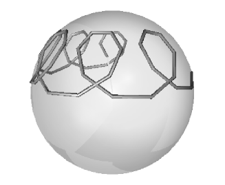
Figure 1: Evolution of the axis of the discrete spinning top

The motion of the discrete time Lagrange top can be viewed using a web–browser. The Java–applet has been written by Ulrich Heller and can be found on the web page

http://www-sfb288.math.tu-berlin.de/~bobenko/bobenko.html

The applet presents an animated spinning top described by the formulas of the present paper.

8 Conclusion

We took an opportunity of elaborating an integrable discretization of the Lagrange top to study in a considerable detail the general theory of discrete time Lagrangian mechanics on Lie groups. We consider this theory as an important source of symplectic and, more general, Poisson maps. Moreover, from some points of view the variational (Lagrangian) structure is even more fundamental and important than the Poisson (Hamiltonian) one (cf. [HMR], [MPS], where a similar viewpoint is represented).

It is somewhat astonishing that this construction is able to produce integrable discrete time systems, since integrability is not built in it a priori. Nevertheless, we extend the Moser–Veselov’s list [V], [MV] of integrable discrete time Lagrangian systems with a new item, namely, an integrable discrete time Lagrange top. It seems that this list may be further continued.

In finding this new discrete time mechanical system an analogy with some differential–geometric notions was very instructive. Also these interrelations between integrable differential geometry and integrable mechanics, both continuous and discrete, deserve to be studied further.

Let us mention also some more concrete problems connected with this work. First of all, the discrete time Lax representations found here call for being understood both from the $r$–matrix point of view [RSTS], [S] and from the point of view of matrix factorizations [MV] (unfortunately, these two schemes, being in principle closely related, still could not be merged into a unified one). Futher, the discrete time dynamics should be integrated in terms of elliptic functions. The methods of the finite–gap theory will be useful here [RM]. Finally, it would be important to elaborate a variational interpretation of different integrable discretizations of the Euler top found in [BLS].

Appendix A Notations

We fix here some notations and definitions used throughout the paper.

Let $G$ be a Lie group with the Lie algebra ${{g}}$, and let ${{g}}^{*}$ be a dual vector space to ${{g}}$. We identify ${{g}}$ and ${{g}}^{*}$ with the tangent space and the cotangent space to $G$ in the group unity, respectively:

$${{g}}=T_{e}G\;,\qquad{{g}}^{*}=T^{*}_{e}G\;.$$

The pairing between the cotangent and the tangent spaces $T^{*}_{g}G$ and $T_{g}G$ in an arbitrary point $g\in G$ is denoted by $\langle\cdot,\cdot\rangle$. The left and right translations in the group are the maps $L_{g}\,,R_{g}\,:G\mapsto G$ defined by

$$L_{g}\,h=gh\;,\qquad R_{g}\,h=hg\qquad\forall h\in G\;,$$

and $L_{g*}\,$, $R_{g*}$ stand for the differentials of these maps:

$$L_{g*}\,:\,T_{h}G\mapsto T_{gh}G\;,\qquad R_{g*}\,:\,T_{h}G\mapsto T_{hg}G\;.$$

We denote by

$${\rm Ad}\,g=L_{g*}R_{g^{-1}*}\,:{{g}}\mapsto{{g}}$$

the adjoint action of the Lie group $G$ on its Lie algebra ${{g}}=T_{e}G$. The linear operators

$$L_{g}^{*}\,:\,T^{*}_{gh}G\mapsto T^{*}_{h}G\;,\qquad R_{g}^{*}\,:\,T^{*}_{hg}G\mapsto T^{*}_{h}G$$

are conjugated to $L_{g*}\,$, $R_{g*}\,$, respectively, via the pairing $\langle\cdot,\cdot\rangle$:

$$\langle L_{g}^{*}\xi,\eta\rangle=\langle\xi,L_{g*}\eta\rangle\quad{\rm for}\quad\xi\in T^{*}_{gh}G\,,\;\;\eta\in T_{h}G\;,$$

$$\langle R_{g}^{*}\xi,\eta\rangle=\langle\xi,R_{g*}\eta\rangle\quad{\rm for}\quad\xi\in T^{*}_{hg}G\,,\;\;\eta\in T_{h}G\;.$$

The coadjoint action of the group

$${\rm Ad}^{*}\,g=L^{*}_{g}R^{*}_{g^{-1}}\,:{{g}}^{*}\mapsto{{g}}^{*}$$

is conjugated to ${\rm Ad}\,g$ via the pairing $\langle\cdot,\cdot\rangle$:

$$\langle{\rm Ad}^{*}\,g\cdot\xi,\eta\rangle=\langle\xi,{\rm Ad}\,g\cdot\eta\rangle\quad{\rm for}\quad\xi\in{{g}}^{*}\,,\;\;\eta\in{{g}}\;.$$

The differentials of ${\rm Ad}\,g$ and of ${\rm Ad}^{*}\,g$ with respect to $g$ in the group unity $e$ are the operators

$${\rm ad}\,\eta\,:{{g}}\mapsto{{g}}\qquad{\rm and}\qquad{\rm ad}^{*}\,\eta\,:{{g}}^{*}\mapsto{{g}}^{*}\;,$$

respectively, also conjugated via the pairing $\langle\cdot,\cdot\rangle$:

$$\langle{\rm ad}^{*}\,\eta\cdot\xi,\zeta\rangle=\langle\xi,{\rm ad}\,\eta\cdot\zeta\rangle\qquad\forall\xi\in{{g}}^{*}\,,\;\;\zeta\in{{g}}\;.$$

The action of ad is given by applying the Lie bracket in ${{g}}$:

$${\rm ad}\,\eta\cdot\zeta=[\eta,\zeta]\;,\quad\forall\zeta\in{{g}}\;.$$

Finally, we shall need the notion of gradients of functions on vector spaces and on manifolds. If ${\cal X}$ is a vector space, and $f:{\cal X}\mapsto{{R}}$ is a smooth function, then the gradient $\nabla f:{\cal X}\mapsto{\cal X}^{*}$ is defined via the formula

$$\langle\nabla f(x),y\rangle=\left.\frac{d}{d\epsilon}\,f(x+\epsilon y)\right|_{\epsilon=0}\;,\qquad\forall y\in{\cal X}\;.$$

Similarly, for a function $f:G\mapsto{{R}}$ on a smooth manifold $G$ its gradient $\nabla f\,:\,G\mapsto T^{*}G$ is defined in the following way: for an arbitrary $\dot{g}\in T_{g}G$ let $g(\epsilon)$ be a curve in $G$ through $g(0)=g$ with the tangent vector $\dot{g}(0)=\dot{g}$. Then

$$\langle\nabla f(g),\dot{g}\rangle=\left.\frac{d}{d\epsilon}\,f(g(\epsilon))\right|_{\epsilon=0}\;.$$

If $G$ is a Lie group, then two convenient ways to define a curve in $G$ through $g$ with the tangent vector $\dot{g}$ are the following:

$$g(\epsilon)=e^{\epsilon\eta}g\;,\quad\eta=R_{g^{-1}*}\,\dot{g}\;,$$

and

$$g(\epsilon)=ge^{\epsilon\eta}\;,\quad\eta=L_{g^{-1}*}\,\dot{g}\;,$$

which allows to establish the connection of the gradient $\nabla f$ with the (somewhat more convenient) notions of the left and the right Lie derivatives of a function $f:G\mapsto{{R}}$:

$$\nabla f(g)=R_{g^{-1}}^{*}\,df(g)=L_{g^{-1}}^{*}\,d\,^{\prime}f(g)\;.$$

Here $df(g):G\mapsto{{g}}^{*}$ and $d\,^{\prime}f(g):G\mapsto{{g}}^{*}$ are defined via the formulas

$$\langle df(g),\eta\rangle=\left.\frac{d}{d\epsilon}\,f(e^{\epsilon\eta}g)\right|_{\epsilon=0}\;,\qquad\forall\eta\in{{g}}\;,$$

$$\langle d\,^{\prime}f(g),\eta\rangle=\left.\frac{d}{d\epsilon}\,f(ge^{\epsilon\eta})\right|_{\epsilon=0}\;,\qquad\forall\eta\in{{g}}\;.$$

Appendix B Lagrangian equations of motion

CONTINUOUS TIME	DISCRETE TIME
General Lagrangian systems
${\bf L}(g,\dot{g})$	${{L}}(g_{k},g_{k+1})$
$\left\{\begin{array}[]{l}\Pi=\nabla_{\dot{g}}{\bf L}\\ \dot{\Pi}=\nabla_{g}{\bf L}\end{array}\right.$	$\left\{\begin{array}[]{l}\Pi_{k}=-\nabla_{1}{{L}}(g_{k},g_{k+1})\\ \Pi_{k+1}=\nabla_{2}{{L}}(g_{k},g_{k+1})\end{array}\right.$
Left trivialization: $\;\;M=L_{g}^{*}\Pi$
${\bf L}(g,\dot{g})={\bf L}^{(l)}(g,\Omega)$	${{L}}(g_{k},g_{k+1})={{L}}^{(l)}(g_{k},W_{k})$
$\Omega=L_{g^{-1}*}\dot{g}$	$W_{k}=g_{k}^{-1}g_{k+1}$
$M=L_{g}^{*}\Pi=\nabla_{\Omega}{\bf L}^{(l)}$	$M_{k}=L_{g_{k}}^{*}\Pi_{k}=d\,^{\prime}_{\!W}{{L}}^{(l)}(g_{k-1},W_{k-1})$
$\left\{\begin{array}[]{l}\dot{M}={\rm ad}^{*}\,\Omega\cdot M+d\,^{\prime}_{\!g}{\bf L}^{(l)}\\ \dot{g}=L_{g*}\Omega\end{array}\right.$	$\left\{\begin{array}[]{l}{\rm Ad}^{*}\,W_{k}^{-1}\cdot M_{k+1}=M_{k}+d\,^{\prime}_{\!g}{{L}}^{(l)}(g_{k},W_{k})\\ g_{k+1}=g_{k}W_{k}\end{array}\right.$
Left trivialization, left symmetry reduction: $\;\;M=L_{g}^{*}\Pi\,,\;\;P={\rm Ad}\,g^{-1}\cdot\zeta$
${\bf L}(g,\dot{g})={\cal L}^{(l)}(P,\Omega)$	${{L}}(g_{k},g_{k+1})=\Lambda^{(l)}(P_{k},W_{k})$
$\Omega=L_{g^{-1}*}\dot{g}\,,\;\;P={\rm Ad}\,g^{-1}\cdot\zeta$	$W_{k}=g_{k}^{-1}g_{k+1}\,,\;\;P_{k}={\rm Ad}\,g_{k}^{-1}\cdot\zeta$
$M=L_{g}^{*}\Pi=\nabla_{\Omega}{\cal L}^{(l)}$	$M_{k}=L_{g_{k}}^{*}\Pi_{k}=d\,^{\prime}_{\!W}\Lambda^{(l)}(P_{k-1},W_{k-1})$
$\left\{\begin{array}[]{l}\dot{M}={\rm ad}^{*}\,\Omega\cdot M+{\rm ad}^{*}\,P\cdot\nabla_{P}{\cal L}^{(l)}\\ \dot{P}=[P,\Omega]\end{array}\right.$	$\left\{\begin{array}[]{l}{\rm Ad}^{*}\,W_{k}^{-1}\cdot M_{k+1}=M_{k}+{\rm ad}^{*}P_{k}\cdot\nabla_{P}\Lambda^{(l)}(P_{k},W_{k})\\ P_{k+1}={\rm Ad}\,W_{k}^{-1}\cdot P_{k}\end{array}\right.$

Right trivialization: $\;\;m=R_{g}^{*}\Pi$
${\bf L}(g,\dot{g})={\bf L}^{(r)}(g,\omega)$	${{L}}(g_{k},g_{k+1})={{L}}^{(r)}(g_{k},w_{k})$
$\omega=R_{g^{-1}*}\dot{g}$	$w_{k}=g_{k+1}g_{k}^{-1}$
$m=R_{g}^{*}\Pi=\nabla_{\omega}{\bf L}^{(r)}$	$m_{k}=R_{g_{k}}^{*}\Pi_{k}=d_{w}{{L}}^{(r)}(g_{k-1},w_{k-1})$
$\left\{\begin{array}[]{l}\dot{m}=-{\rm ad}^{*}\,\omega\cdot m+d_{g}{\bf L}^{(r)}\\ \dot{g}=R_{g*}\omega\end{array}\right.$	$\left\{\begin{array}[]{l}{\rm Ad}^{*}\,w_{k}\cdot m_{k+1}=m_{k}+d_{g}{{L}}^{(r)}(g_{k},w_{k})\\ g_{k+1}=w_{k}g_{k}\end{array}\right.$
Right trivialization, right symmetry reduction: $\;\;m=R_{g}^{*}\Pi\,,\;\;a={\rm Ad}\,g\cdot\zeta$
${\bf L}(g,\dot{g})={\cal L}^{(r)}(a,\omega)$	${{L}}(g_{k},g_{k+1})=\Lambda^{(r)}(a_{k},w_{k})$
$\omega=R_{g^{-1}*}\dot{g}\,,\;\;a={\rm Ad}\,g\cdot\zeta$	$w_{k}=g_{k+1}g_{k}^{-1}\,,\;\;a_{k}={\rm Ad}\,g_{k}\cdot\zeta$
$m=R_{g}^{*}\Pi=\nabla_{\omega}{\cal L}^{(r)}$	$m_{k}=R_{g_{k}}^{*}\Pi_{k}=d_{w}\Lambda^{(r)}(a_{k-1},w_{k-1})$
$\left\{\begin{array}[]{l}\dot{m}=-{\rm ad}^{*}\,\omega\cdot m-{\rm ad}^{*}\,a\cdot\nabla_{a}{\cal L}^{(r)}\\ \dot{a}=[\omega,a]\end{array}\right.$	$\left\{\begin{array}[]{l}{\rm Ad}^{*}\,w_{k}\cdot m_{k+1}=m_{k}-{\rm ad}^{*}a_{k}\cdot\nabla_{a}\Lambda^{(r)}(a_{k},w_{k})\\ a_{k+1}={\rm Ad}\,w_{k}\cdot a_{k}\end{array}\right.$

The relation between the continuous time and the discrete time equations is established, if we set

$$g_{k}=g\;,\qquad g_{k+1}=g+\varepsilon\dot{g}+O(\varepsilon^{2})\;,\qquad{{L}}(g_{k},g_{k+1})=\varepsilon{\bf L}(g,\dot{g})+O(\varepsilon^{2})\;;$$

$$P_{k}=P\;,\qquad W_{k}={\bf 1}+\varepsilon\Omega+O(\varepsilon^{2})\;,\qquad\Lambda^{(l)}(P_{k},W_{k})=\varepsilon{\cal L}^{(l)}(P,\Omega)+O(\varepsilon^{2})\;;$$

$$a_{k}=a\;,\qquad w_{k}={\bf 1}+\varepsilon\omega+O(\varepsilon^{2})\;,\qquad\Lambda^{(r)}(a_{k},w_{k})=\varepsilon{\cal L}^{(r)}(a,\omega)+O(\varepsilon^{2})\;.$$

Appendix C On $SU(2)$ and $su(2)$

The Lie group $G=SU(2)$ consists of complex $2\times 2$ matrices $g$ satisfying the condition $gg^{*}=g^{*}g={\bf 1}$, where ${\bf 1}$ is the group unit, i.e. the $2\times 2$ unit matrix, and ^∗ denotes the Hermitean conjugation, i.e. $g^{*}=\bar{g}^{T}$. In components:

$$g=\left(\begin{array}[]{cc}\alpha&\beta\\ -\bar{\beta}&\bar{\alpha}\end{array}\right)=\left(\begin{array}[]{cc}a+ib&c+id\\ -c+id&a-ib\end{array}\right)\;,$$ (C.1)

where

$$\alpha=a+ib\,,\;\beta=c+id\in{{C}}\;,$$

and

$$|\alpha|^{2}+|\beta|^{2}=a^{2}+b^{2}+c^{2}+d^{2}=1\;.$$ (C.2)

The tangent space $T_{e}SU(2)$ is the Lie algebra ${{g}}=su(2)$ consisting of complex $2\times 2$ matrices $\eta$ such that $\eta+\eta^{*}=0$. In components,

$$\eta=\left(\begin{array}[]{cc}ib&c+id\\ -c+id&-ib\end{array}\right)\;.$$ (C.3)

The Lie bracket in $su(2)$ is the usual matrix commutator.

Let us introduce the following notations: for an arbitrary matrix $g$ of the form (C.1), not necessary belonging to $SU(2)$, set

$$\Re(g)=\left(\begin{array}[]{cc}a&0\\ 0&a\end{array}\right)\;,\quad\Im(g)=\left(\begin{array}[]{cc}ib&c+id\\ -c+id&-ib\end{array}\right)\;,$$

so that $\Re(g)$ is a scalar real matrix, and $\Im(g)\in su(2)$.

As it is always the case for matrix groups, we have for $g\in SU(2)$, $\eta\in su(2)$:

$$L_{g*}\eta=g\eta\;,\quad R_{g*}\eta=\eta g\;,\quad{\rm Ad}\,g\cdot\eta=g\eta g^{-1}\;.$$ (C.4)

If we write (C.3) as

$$\eta=\frac{1}{2}\left(\begin{array}[]{cc}-i\eta_{3}&-\eta_{2}-i\eta_{1}\\ \eta_{2}-i\eta_{1}&i\eta_{3}\end{array}\right)\;,$$ (C.5)

and put this matrix in a correspondence with the vector

$$\eta=(\eta_{1},\eta_{2},\eta_{3})^{T}\in{{R}}^{3}\;,$$

then it is easy to verify that this correspondence is an isomorphism between $su(2)$ and the Lie algebra $\Big{(}{{R}}^{3},\,\times\Big{)}$, where $\times$ stands for the vector product. This allows not to distinguish between vectors from ${{R}}^{3}$ and matrices from $su(2)$. In other words, we use the following basis of the linear space $su(2)$:

$${\bf e}_{1}=\frac{1}{2}\left(\begin{array}[]{cc}0&-i\\ -i&0\end{array}\right)=\frac{1}{2i}\,\sigma_{1}\;,\qquad{\bf e}_{2}=\frac{1}{2}\left(\begin{array}[]{cc}0&-1\\ 1&0\end{array}\right)=\frac{1}{2i}\,\sigma_{2}\;,$$

$${\bf e}_{3}=\frac{1}{2}\left(\begin{array}[]{cc}-i&0\\ 0&i\end{array}\right)=\frac{1}{2i}\,\sigma_{3}\;,$$ (C.6)

where $\sigma_{j}$ are the Pauli matrices.

We supply $su(2)$ with the scalar product $\langle\cdot,\cdot\rangle$ induced from ${{R}}^{3}$. It is easy to see that in the matrix form it may be represented as

$$\langle\eta,\zeta\rangle=-2\,{\rm tr}(\eta\zeta)=2\,{\rm tr}(\eta\zeta^{*})\;.$$ (C.7)

This scalar product allows us to identify the dual space $su(2)^{*}$ with $su(2)$ itself, so that the coadjoint action of the algebra becomes the usual Lie bracket with minus:

$${\rm ad}^{*}\,\eta\cdot\xi=[\xi,\eta]=-{\rm ad}\,\eta\cdot\xi\;.$$ (C.8)

We use a formula similar to (C.7) to define a scalar product of two arbitrary complex $2\times 2$ matrices:

$$\langle g_{1},g_{2}\rangle=2\,{\rm tr}(g_{1}g_{2}^{*})\;.$$ (C.9)

(In particular, the square of the norm of every matrix $g\in SU(2)$ is equal to 4). The formula (C.9) gives us a left– and right–invariant scalar product in all tangent spaces $T_{g}G$. Indeed, to see, for instance, the left invariance, let $g\eta,g\zeta\in T_{g}SU(2)$ (here $g\in SU(2)$, $\eta,\zeta\in su(2)$). Then

$$\langle g\eta,g\zeta\rangle=2\,{\rm tr}(g\eta\zeta^{*}g^{*})=2\,{\rm tr}(\eta\zeta^{*})=\langle\eta,\zeta\rangle\;.$$

This scalar product allows to identify the cotangent spaces $T^{*}_{g}G$ with the tangent spaces $T_{g}G$. It follows easily that:

$$L_{g}^{*}\xi=g^{-1}\xi\;,\quad R_{g}^{*}\xi=\xi g^{-1}\;,\quad{\rm Ad}^{*}\,g\cdot\xi=g^{-1}\xi g\;.$$ (C.10)

(in these formulas $g\in SU(2)$, so that $g^{-1}=g^{*}$).

Let us now formulate several simple properties of $SU(2)$ and $su(2)$ which will be used later on.

Lemma C.1

For an arbitrary $g\in SU(2)$:

$$g=\cos(\theta)\,{\bf 1}+\sin(\theta)\,\zeta\qquad{\rm with}\qquad\zeta\in su(2)\;,\quad\langle\zeta,\zeta\rangle=4\;.$$ (C.11)

The adjoint action of $SU(2)$ on $su(2)$ has in these notations the following geometrical interpretation: $g\eta g^{-1}$ is a rotation of the vector $\eta$ around the vector $\zeta$ by the angle $2\theta$.

This interpretation makes $SU(2)$ very convenient for describing rotations in ${{R}}^{3}$ (in some respects more convenient than the standard use of $SO(3)$ in this context). Since by rotations only the vectors on the rotation axis remain fixed, we see that for the case $G=SU(2)$

$$G^{[\zeta]}=G^{(\zeta)}\;.$$

In a different way, the previous lemma may be formulated as follows.

Lemma C.2

For $g\in SU(2)$, if

$$2\,\frac{\Im(g)}{{\rm tr}(g)}=\xi\;,$$ (C.12)

then

$$g=\frac{{\rm tr}(g)}{2}\,({\bf 1}+\xi)\;,\qquad{\rm tr}(g)=\frac{2}{\sqrt{1+\langle\xi,\xi\rangle/4}}\;.$$ (C.13)

We have also the following simple connection between the matrix multiplication and the commutator in $su(2)$ .

Lemma C.3

For $\eta,\zeta\in su(2)$ their matrix product has the form (C.1), and

$$\eta\zeta=-\frac{1}{4}\,\langle\eta,\zeta\rangle{\bf 1}+\frac{1}{2}\,[\eta,\zeta]\;.$$ (C.14)

In particular, the following corollary is important:

$$\langle\eta,\zeta\rangle=0\;\Rightarrow\;\eta\zeta=-\zeta\eta\;.$$ (C.15)

References

- [AL] M.Ablowitz, J.Ladik. A nonlinear difference scheme and inverse scattering. Stud. Appl. Math. 55 (1976) 213–229; On solution of a class of nonlinear partial difference equations. Stud. Appl. Math. 57 (1977) 1–12.
- [AM] M.Adler, P.van Moerbeke. Completely integrable systems, Euclidean Lie algebras and curves. Adv. Math. 38 (1980) 267–317.
- [A] V.I.Arnold. Mathematical methods of classical mechanics. Springer, 1978.
- [Au] M.Audin. Spinning tops. Cambridge University Press, 1996.
- [B] A.I.Bobenko. Discrete integrable systems and geometry. Proc. Int. Congress Math. Phys. ’97 (to appear).
- [BLS] A.I.Bobenko, B.Lorbeer, Yu.B.Suris. Integrable discretizations of the Euler top. J. Math. Phys. (1998, to appear).
- [BP] A.I.Bobenko, U.Pinkall. Discretization of surfaces and integrable systems. – In: Discrete integrable geometry and physics, Eds. A.Bobenko and R.Seiler, Oxford University Press, 1998.
- [CB] R.H.Cushman, L.M.Bates. Global aspects of classical integrable systems. Birkhäuser, 1997.
- [DJM] F.Date, M.Jimbo, and T.Miwa. Method for generating discrete soliton equations. I–IV. J. Phys. Soc. Japan 51 (1982) 4116–4124, 4125–4131; 52 (1983) 761–765, 766–771.
- [DS] A.Doliwa, P.Santini. Geometry of discrete curves and lattices and integrable difference equations. – In: Discrete integrable geometry and physics, Eds. A.Bobenko and R.Seiler, Oxford University Press, 1998.
- [FT] L.D.Faddeev, L.A.Takhtadjan. Hamiltonian methods in the theory of solitons, Springer, 1987.
- [G] V.V.Golubev. Lectures on the integration of the equations of motion of a rigid body about a fixed point. State Publishing, Moscow, 1953.
-
[Ha]
H.Hasimoto. Motion of a vortex filament and its relation
to elastica. J. Phys. Soc. Japan 31 (1971) 293–294;
A soliton of a vortex filament. J. Fluid Mech. 51 (1972) 477–485. - [H] R.Hirota. Nonlinear partial difference equations. I–V. J. Phys. Soc. Japan 43 (1977) 1423–1433, 2074–2078, 2079–2086; 45 (1978) 321–332; 46 (1978) 312–319.
- [HMR] D.D.Holm, J.E.Marsden, T.Ratiu. The Euler–Poincare equations and semidirect products with applications to continuum theories. Adv. Math. (1998, to appear).
- [KS] F.Klein, A.Sommerfeld. Über die Theorie des Kreisels. Teubner, 1965. (Reprint of the 1897–1910 edition).
- [L] A.E.H.Love. A treatize of the mathematical theory of elasticity. Cambridge, 1892.
- [LS] J.Langer, D.Singer. Lagrangian aspects of the Kirchhoff elastic rod. SIAM Rev. 38 (1996) 605–618.
- [MPS] J.E.Marsden, G.W.Patrick, S.Shkoller. Multisymplectic geometry, variational integrators, and nonlinear PDEs. Commun. Math. Phys. (1998, to appear).
- [MR] J.E.Marsden, T.S.Ratiu. Introduction to mechanics and symmetry. Springer, 1994.
- [MRW] J.E.Marsden, T.S.Ratiu, A.Weinstein. Semi–direct products and reduction in mechanics. Trans. Am. Math. Soc. 281 (1984) 147–177; Reduction and Hamiltonian structures on duals of semidirect products Lie algebras. Contemp. Math. 28 (1984) 55–100.
-
[MS]
J.E.Marsden, J.Scheurle. Lagrangian reduction and the
double spherical pendulum. ZAMP 44 (1993) 17–43;
The reduced Euler–Lagrange equations. Fields Inst. Comm. 1 (1993) 139–164. - [MV] J.Moser, A.P.Veselov. Discrete versions of some classical integrable systems and factorization of matrix polynomials. Commun. Math. Phys. 139 (1991) 217–243.
- [QNCV] G.Quispel, F.Nijhoff, H.Capel, and J.Van der Linden Linear integral equations and nonlinear differential–difference equations. Physica A 125 (1984) 344–380.
- [RM] T.Ratiu, P.van Moerbeke. The Lagrange rigid body motion. Ann. Inst. Fourier 32 (1982) 211–234.
- [R] A.G.Reyman. Integrable Hamiltonian systems connected with graded Lie algebras. J. Sov. Math. 19 (1982) 1507–1545.
- [RSTS] A.G.Reyman, M.A.Semenov-Tian-Shansky. Group theoretical methods in the theory of finite dimensional integrable systems. In: Encyclopaedia of mathematical science, v.16: Dynamical Systems VII, Springer, 1994, 116–225.
- [Skl] E.K.Sklyanin. On some algebraic structures related to the Yang–Baxter equation. Fuct. Anal. and Appl. 16 (1982) 27–34.
- [S] Yu.B.Suris. –matrices and integrable discretizations. – In: Discrete integrable geometry and physics, Eds. A.Bobenko and R.Seiler, Oxford University Press, 1988.
- [V] A.P.Veselov. Integrable systems with discrete time and difference operators. Funct. Anal. Appl. 22 (1988) 1–13.
- [WM] J.M.Wendlandt, J.E.Marsden. Mechanical integrators derived from a discrete variational principle. Physica D 106 (1997) 223–246.