The Whitham Equations for
Optical Communications:
Mathematical Theory of NRZ

Abstract

We present a model of optical communication system for high-bit-rate data transmission in the nonreturn-to-zero (NRZ) format over transoceanic distance. The system operates in a small group velocity dispersion regime, and the model equation is given by the Whitham equations describing the slow modulation of multi-phase wavetrains of the (defocusing) nonlinear Schrödinger (NLS) equation. The model equation is of hyperbolic type, and certain initial NRZ pulse with phase modulation develops a shock. We then show how one can obtain a global solution by choosing an appropriate Riemann surface on which the Whitham equation is defined. The present analysis may be interpreted as an alternative to the method of inverse scattering transformation for the NLS solitons. We also discuss wavelength-division-multiplexing (WDM) in the NRZ format by using the Whitham equation for a coupled NLS equation, and show that there exists a hydro-dynamic-type instability between channels.

1 Introduction

Recently there has been a great deal of research works on designing a long-distance and high-speed optical communication system for the next generation of 100Gbit/s over 9000km (transpacific distance). In the fall of 1996, the undersea optical cable called TPC-5 between Japan and US has been installed, and the system operates at 10Gbit/s in a non-return-to-zero (NRZ) format. Also in 1998, a total of 100Gbit/s (e.g. 5Gbit/s $\times$ 20Channels) wavelength-division-multiplexed (WDM)-NRZ system will be set up as TPC-6 optical cable. In such a system, noise accumulation and the combined action of fiber dispersion in the group velocity of pulse and fiber nonlinearity called the Kerr effect are the main system limiting factors. The analysis of NRZ signal propagation was hampered so far by necessity of lengthy numerical simulation and expensive experiments. Recently, we proposed in [14] a hydrodynamic model to describe nonlinear effects in the NRZ pulse propagation, which was derived as a weak dispersion limit of the nonlinear Schrödinger (NLS) equation. Based on this model, we also discussed methods to control the pulse broadening by means of initial phase modulation (pre-chirping) [15] and nonlinear gain [16].

In this paper, we give a mathematical formulation of the model in the framework of the Whitham averaging method [25] which describes the slow modulation of the amplitude and phase of quasi-periodic solution of the NLS equation. We start in Section 2 to provide a necessary information of the problem, and derive a shallow water wave equation as a simplest approximation of the model. In Section 3, we give a mathemtical background of the Whitham equation as describing dynamics of the genus $g$ Riemann surface determined by the spectral curve of the Lax operator for the NLS equation. Here the genus represents the number of periods in the quasi-periodic solution, and the Whitham equations are given by first order quasi-linear system of partial differential equations. In particular, we identify the shallow water wave equation as the genus zero Whitham equation. We also note that the spectral curves corresponding to the Whitham equation for the NLS equation (NLS-Whitham equation) are hyper-elliptic. In Section 4, we first show the hyperbolicity of the NLS-Whitham equations which enables us to classify the initial data for the global existence of the solution. We then decribe the effect of pre-chirping for reducing the broadening of NRZ pulse, and as a result we find that the Riemann surface becomes singular (formation of a shock), and its genus changes from zero to either one or two depending on the strength of the chirp.

Since the NRZ system operates at a small group velocity (i.e. second order) dispersion regime, the third order dispersion becomes important, especially for pulses with shorter width (in a higher bit rate system). We discuss this effect in Section 5, and show that the third order dispersion leads to asymmetric distortion of the NRZ pulse and results a formation of shock-like structure. In Section 6, we extend the NLS-Whitham model to describe pulse propagation in a WDM-NRZ system. The extension is obtained by taking a weak dispersion limit of a coupled NLS equation, in which the interaction between channels due to the Kerr nonlinearity is expressed by the cross phase modulation. We then find a hydrodynamic-type instability between channels, which corresponds to loosing the hyperbolicity of the hydrodynamic model obtained in the dispersionless limit of this coupled NLS equations. The WDM model is further studied by using an integrable model, the Manakov equation [20] or the vector NLS equation. The Whitham equation of genus zero in this model is the well-known Benney equation which describes shallow water waves in a stratified fluids [2, 27], and the number of channels in WDM corresponds to that of the layers. We then present how the nonzero genus Whitham equations appear in the Manakov equation. The main feature of this model is that the spectral curve is non-hyperelliptic, and the corresponding generic Riemann surface has a topology of a sphere with $3h$ handles with some positive integer $h$.

2 Preliminary

For a long-distance and high-bit rate optical communication system, both dispersion and nonlinearity of the optical fiber are important and the NLS equation has been used as a model equation expressing such effects [9],

$$i{{{\partial}q}\over{{\partial}Z}}+{\beta_{2}\over 2}{{{\partial}^{2}q}\over{{\partial}T^{2}}}+\nu|q|^{2}q = 0,$$ (2.1)

Here $q$ is the complex envelope function of the electric field in the fiber, $Z$ the propagation distance, and $T$ the retarded time. The coefficients $\beta_{2}$ and $\nu(>0)$ represent the group velocity dispersion (GVD) and the Kerr (nonlinear) effect of the fiber. Here we further normalize $q$ so that we can set $\nu=1$. It is well known that if ${\beta}_{2}>0$ (focusing or modulationally unstable case), the NLS equation has so-called bright solitons with sech-shape, and if ${\beta}_{2}<0$ (deforcusing or modulationally stable case), so-called dark ones with tanh-shape. These are the stationary solutions for Eq.(2.1), and Fig.1 shows examples of pulse sequences in $|q|^{2}$ as a 16bits-coded signal (0010110010111100) using those pulses.

Figure 1: Various types of a 16bits coded signal (0010110010111100).

In Fig.1, we also show the coded signal using the NRZ pulses. Because of the modulational stability of constant amplitude, for example, in the (011110) coding part, one has to operate the NRZ system at the deforcusing regime, $\beta_{2}<0$. The NRZ pulse is however non-stationary, and in order to reduce the pulse distortion the system is designed in a small dispersion and low power regime. In an ideal case, the best performance can be obtained in the zero dispersion and linear limits. However, the real system always includes a noise, and the signal pulse power should be kept more than the noise level. Because of this limit in signal-noise ratio (SNR), the nonlinearity becomes an essential effect for a long distance transmission problem, and the zero dispersion causes a resonant interaction process between noise and signal, which is called the four wave mixing (FWM), and leads to a distortion of the pulse. The main purpose of this paper is to develop a mahematical theory to describe the pulse distortion in a weak dispersion limit of the NLS equation. Here we do not discuss, however, the distortion due to the FWM with noise.

Let us first recall that the NLS equation (2.1) has an infinite number of conservation laws, for example,

$$\frac{\partial}{\partial Z}|q|^{2}=\frac{\partial}{\partial T}\left(\beta^{2}|q|^{2}\frac{\partial}{\partial T}\mbox{Arg}(q)\right),$$ (2.2)

$$\frac{\partial}{\partial Z}\left(|q|^{2}\frac{\partial}{\partial T}\mbox{Arg}(q)\right)=\frac{\partial}{\partial T}\left(-\frac{\beta^{2}}{4}\frac{\partial^{2}q}{\partial T^{2}}+\beta^{2}\left|\frac{\partial q}{\partial T}\right|^{2}+\frac{1}{2}|q|^{4}\right).$$ (2.3)

Here we have set $\beta_{2}=-{\beta}^{2}$. The quantities $|q|^{2}$ and Arg($q$)$:=(i/2)\ln(q^{*}/q)$ represent the local intensity and phase of the electric field. We then introduce $\rho:=|q|$ and $\sigma:=\beta$Arg($q$), and rewrite $q$ as

$$q(T,Z)=\sqrt{\rho(T,Z)}\exp\left(i\frac{1}{\beta}{\sigma}(T,Z)\right).$$ (2.4)

Substituting Eq.(2.4) to Eqs.(2.2) and (2.3), and rescaling the variables $Z\rightarrow Z/{\beta}$, we have

$$\frac{\partial}{\partial Z}\rho=\frac{\partial}{\partial T}\left(\rho u\right),$$ (2.5)

$$\frac{\partial}{\partial Z}\left(\rho u\right)=\frac{\partial}{\partial T}\left(\rho u^{2}+\frac{1}{2}\rho^{2}-\frac{\beta^{2}}{4}\rho\frac{\partial^{2}}{\partial T^{2}}\ln\rho\right).$$ (2.6)

where $u$ represents the chirp defined by $u:=\partial\sigma/\partial T$. In a small dispersion limit ${\beta}\rightarrow 0$, if we assume that both $\rho$ and $u$ are smooth, then Eqs.(2.5) and (2.6) for $\rho\neq 0$ can be approximated by a $2\times 2$ quasi-linear system,

$${{\partial}\over{{\partial}Z}}\left(\matrix{\rho\cr u\cr}\right) = \left(\matrix{u&\rho\cr 1&u\cr}\right){{\partial}\over{{\partial}T}}\left(\matrix{\rho\cr u\cr}\right).$$ (2.7)

A detail on the weak dispersion limit of the NLS equation has been studied in [10], where the existence theorem of the limit is given based on the Lax-Levermore theory. When $\rho>0$ in (2.7), the eigenvalues of the coefficient matrix are real, $u+\sqrt{\rho}$ and $u-\sqrt{\rho}$, and the system is totally hyperbolic. The system (2.7) is known as the shallow water wave equation, and has been intensively discussed (for example, see [25]). It is then interesting to note that the distortion of the NRZ pulse may be understood as a deformation of the water surface.

For a demonstration of the NRZ pulse propagation, we consider the initial value problem of Eq.(2.7). As a simple example of the initial NRZ pulse, we take a square pulse having constant phase (zero-chirp),

$$\rho(T,0)=\left\{\begin{array}[]{ll}\rho_{0},&\mbox{for~{}~{} $|T|<T_{0}$}\\ 0,&\mbox{for~{}~{} $|T|>T_{0}$}\end{array}\right.\ ,~{}~{}~{}~{}~{}~{}u(T,0)=0,\ \ \mbox{for~{}~{} $\forall T$}.$$ (2.10)

This is called ”Dam-breaking problem”, since $\rho$ and $-u$ represent the depth and the velocity of water which rests on the spatial region $|T|<T_{0}$ at the time $Z=0$. We then expect to see a leakage of the water from the edges, and in fact we obtain:

Proposition 2.1

The system (2.7) with the initial data (2.10) has the following global solution up to the distance $Z=T_{0}/\sqrt{\rho_{0}}$: For $T>0$,

$$\rho(T,Z) = u(T,Z)=0,\ \ ~{}~{}~{}~{}~{}~{}~{}~{}~{}~{}~{}\mbox{for}\ \ T>T_{0}+2\sqrt{\rho_{0}}Z,$$

$$\rho(T,Z) = \mbox{min}\left[\rho_{0},\frac{1}{9}\left(2\sqrt{\rho_{0}}-\frac{T-T_{0}}{Z}\right)^{2}\right],\ \ \mbox{for }\ \ 0<T<T_{0}+2\sqrt{\rho_{0}}Z,$$

$$u(T,Z) = -\mbox{max}\left[0,{2\over 3}\left(\sqrt{\rho_{0}}+{T-T_{0}\over Z}\right)\right],\ \ ~{}\mbox{for }\ \ 0<T<T_{0}+2\sqrt{\rho_{0}}Z,$$

For $T<0$, we have $\rho(T,Z)=\rho(-T,Z)$ and $u(T,Z)=-u(-T,Z)$.

Proof. As in the standard analysis of the method of characteristics for the quasi-linear hyperbolic system (2.7), we first rewrite the system in the Riemann invariant form [25]

$${{\partial}\over{{\partial}Z}}\left(\matrix{{\lambda}_{1}\cr{\lambda}_{2}\cr}\right) = {1\over 4}\left(\matrix{3{\lambda}_{1}+{\lambda}_{2}&0\cr 0&{\lambda}_{1}+3{\lambda}_{2}\cr}\right){{\partial}\over{{\partial}T}}\left(\matrix{{\lambda}_{1}\cr{\lambda}_{2}\cr}\right),$$ (2.11)

where the Riemann invariants ${\lambda}_{1}$ and ${\lambda}_{2}$ are given by

$${\lambda}_{1}=u-2\sqrt{\rho},~{}~{}~{}~{}~{}{\lambda}_{2}=u+2\sqrt{\rho}.$$ (2.12)

Then the initial data for the Riemann invariants are given by

$${\lambda}_{1}(T,0)=\left\{\begin{array}[]{ll}2\sqrt{\rho_{0}},&\mbox{for~{}~{}~{} $T<-T_{0}$}\\ -2\sqrt{\rho_{0}},&\mbox{for~{}~{}~{} $T>-T_{0}$}\end{array}\right.,$$ (2.15)

(2.16)

$${\lambda}_{2}(T,0)=\left\{\begin{array}[]{ll}2\sqrt{\rho_{0}},&\mbox{for~{}~{}~{} $T<T_{0}$}\\ -2\sqrt{\rho_{0}},&\mbox{for~{}~{}~{} $T>T_{0}$}\end{array}\right..$$ (2.19)

Here we extend the values of $\lambda_{1}$ and $\lambda_{2}$ for the region $|T|>T_{0}$. One should note from Eq.(2.6) that $u$ is defined only the region where $\rho\neq 0$. Then Eq.(2.11) becomes a single equation for $\lambda_{2}$ near $T=T_{0}$ where $\lambda_{1}=-2\sqrt{\rho_{0}}$,

$$\frac{\partial\lambda_{2}}{\partial Z}=\frac{1}{4}(-2\sqrt{\rho_{0}}+3\lambda_{2})\frac{\partial\lambda_{2}}{\partial T},$$ (2.20)

from which we have the solution expressing a rarefaction (centered simple) wave starting from $T=T_{0}$; for $T>0$,

$${\lambda}_{2}(T,Z)=\left\{\begin{array}[]{lll}\displaystyle{2\sqrt{\rho_{0}}},&\mbox{for~{}~{}~{} $0<T<T_{0}-\sqrt{\rho_{0}}Z$},\\ \displaystyle{\frac{2}{3}\sqrt{\rho_{0}}-\frac{4}{3}\frac{T-T_{0}}{Z}},&\mbox{for~{}~{} $T_{0}-\sqrt{\rho_{0}}Z<T<T_{0}+2\sqrt{\rho_{0}}Z$},\\ \displaystyle{-2\sqrt{\rho_{0}}},&\mbox{for~{}~{}~{} $T>T_{0}+2\sqrt{\rho_{0}}Z$}.\end{array}\right.$$ (2.21)

This solution is valid up to the distance $Z=T_{0}/\sqrt{\rho_{0}}$ where the centered simple waves from $T=T_{0}$ and $-T_{0}$ collide at $T=0$, and the solution should be modified. To find ${\lambda}_{1}(T,Z)$, note that the point symmetry in the graphs (${\lambda}_{k},T$), i.e. ${\lambda}_{2}(T)=-{\lambda}_{1}(-T)$. Then from ${\lambda}_{1}$ and ${\lambda}_{2}$ we have the solutions

$$\rho=\frac{1}{16}({\lambda}_{1}-{\lambda}_{2})^{2},~{}~{}~{}~{}~{}~{}u=\frac{1}{2}({\lambda}_{1}+{\lambda}_{2}).$$ (2.22)

Noting the symmetry $\rho(-T,Z)=\rho(T,Z)$ and $u(-T,Z)=-u(T,Z)$, we complete the proof.        

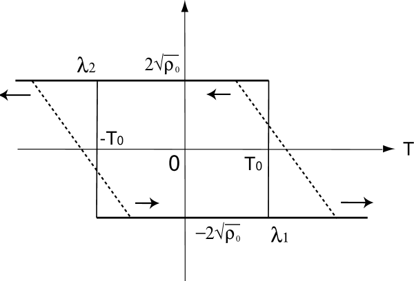
Figure 2: Evolution of the Riemann invariants. Dashed curves are the initial data: Solid curves are the solution ${\lambda}_{k}(T,Z)$ for $Z>0$.

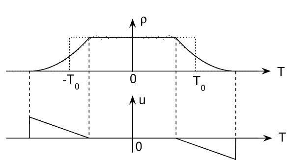
Figure 3: Deformation of NRZ pulse (Dam breaking problem). The thin dotted curve on $\rho$ shows the numerical solution of the NLS equation.

The evolution of the Riemann invariants ${\lambda}_{1}$ and ${\lambda}_{2}$ is shown in Fig.2. In Fig.3, we plot the pulse shape $\rho$ and the chirp $u$ obtained in Proposition 2.1. The thin dotted curve in Fig.3 shows the numerical result of the NLS equation with $\rho_{0}=1,T_{0}=10$ and $\beta_{2}\equiv-\beta^{2}=-0.1$ at $Z=10\beta\approx 3.16$. Notice the good agreement with the analytical solution except some small oscillations on the top of $\rho$ which disappear in the limit $\beta_{2}\to 0$. As we have predicted from the hydrodynamic analogy, the deformation of the pulse induces the generation of chirp (or water velocity) at the edges, and the global nature of the solution is understood as an expansion of the water (the rarefaction wave). The expansion is characterized by the characteristic velocity $s$ at the edge, and for example at $T=T_{0}$ it is given by $s=-\sqrt{\rho_{0}}$ for $T<T_{0}$ and $s=2\sqrt{\rho_{0}}$ for $T>T_{0}$. In order to reduce the expansion, it is natural to put initial chirp opposed to the chirp appearing in the edges. This is equivalent to give an initial velocity with a piston and to compress the water. Because of the quasi-linearity of the system (2.7), we then expect a shock formation in the solution, and therefore Eq.(2.7) is no longer valid as an approximate model of the NLS equation. In fact, if we start with the initial data with the same $\rho$ in (2.10) but nonzero chirp $u$, for example, with $u_{0}>0$

$$u(T,0)=\left\{\begin{array}[]{ll}-u_{0},{}{}&\mbox{for~{}~{}~{} $T<0$}\\ u_{0},{}{}&\mbox{for~{}~{}~{} $T>0$}\end{array}\right.,$$ (2.23)

the numerical solution of the NLS equation results high oscillations starting from the discontinuous point of chirp, $T=0$, as seen in Fig.4.

Figure 4: Optical shock due to initial chirp.

Here we have set $\rho_{0}=1,u_{0}=3\beta\approx 0.95$ with $\beta_{2}=-0.1$, and the solution $\rho(T,Z)$ is at $Z=5\beta\approx 1.58$. This phenomena has been also noted in [5] as an optical shock appearing in somewhat similar situation. The main frequency of the oscillations is of order $1/\beta$, and usual optical filter can remove those oscillations as in the sense of averaging. So what we want to describe here is the average behavior of the solution. For this purpose, in the following section we extend the model (2.7) and show that the new model admits a global solution describing the average motion of the NLS equation (2.1) for several step initial data having different values of chirp. This is the main purpose of the present paper, and it may be referred as a dispersive regularization problem of the shock singularity of hyperbolic system in a weak dispersion limit of the NLS equation.

3 The NLS-Whitham equations

We here develop a regularization method based on the integrability of the NLS equation. The key idea is to identify the shock singularity as a generation of a quasi-periodic solution of the NLS equation which appears as the high oscillations as seen in Fig.4. The quasi-periodic solution can be characterized by the Riemann surface defined by the spectral curve of the Lax operator in the inverse scattering transform (IST). Then the genus of the Riemann surface changes through the singularity. Here the number of the genus corresponds to that of independent phases in the quasi-periodic solution [7, 22]. Then the main purpose here is to derive an equation to describe the dynamics of the Riemann surface corresponding to the modulation of the quasi-periodic solution of the NLS equation. The resulting equation is called the NLS-Whitham equation.

Let us first recall the IST scheme of the NLS equation and reformulate the quasi-linear system (2.7) as the simplest approximation of the NLS equation in a weak dispersion limit, that is, the genus zero NLS-Whitham equation. Then we discuss the  general case with arbitrary genus. Here we somewhat use a different formulation of the IST method, which is related to Sato’s formulation of the KP hierarchy [23]. This is quite useful not only for the present purpose but also for an integrable extension of coupled NLS equation used as a model of WDM system discussed in Section 6. The Lax operator $L$ of the NLS equation in this formulation is given by a pseudo-differential operator with $D:=-i\beta{\partial}/{\partial}T$,

$$L = D+\sqrt{\rho}(D-u)^{-1}\sqrt{\rho}$$ (3.1)

$$= D+\rho D^{-1}+\left(\rho u-{1\over 2}D\rho\right)D^{-2}+\cdots\ .$$

This can be derived from the standard Lax operator in a $2\times 2$ matrix form [26], and the operation with $D^{\ell}$ is given by a generalized Leibnitz rule with $DD^{-1}=D^{-1}D=1$,

$$D^{\ell}f\cdot=\sum_{k=0}^{\infty}\left(\matrix{\ell\cr k\cr}\right)(D^{k}f)D^{\ell-k}\cdot\ \ ,\ \ \mbox{for \ any}\ \ell\in{\bf Z}.$$ (3.2)

Then the IST scheme (the Lax pair) for the NLS equation is given by the eigenvalue problem $L\phi={\lambda}\phi$ and the evolution equation,

$$-i{{{\partial}\phi}\over{{\partial}Z}}=B_{2}\phi,~{}~{}~{}~{}B_{2}={1\over 2}(L^{2})_{\geq 0}:={1\over 2}D^{2}+\rho.$$ (3.3)

Here the symbol $(L^{2})_{\geq 0}$ denotes the differential (i.e. polynomial in $D$) part of the pseudo-differential operator $L^{2}$.

As a genelarization of this scheme, the integrable hierarchy of the NLS equation can be formulated as

$$-i{{{\partial}\phi}\over{{\partial}Z_{n}}}=B_{n}\phi,~{}~{}~{}~{}B_{n}={1\over n}(L^{n})_{\geq 0},$$ (3.4)

where $Z_{n}$ is the parameter describing the evolution generated by $B_{n}$ for $n=1,2,\cdots$. In particular, $Z_{1}$ represents the translation in $T$, that is, $\phi(T,Z_{1},Z_{2},\cdots)=\phi(T+\beta Z_{1},Z_{2},\cdots)$ so that we identify $\beta Z_{1}$ as $T$, and $Z_{3}$ represents the parameter for the complex modified KdV equation which will play an important rule in Section 5 where we discuss a higher order correction to the NLS equation. The compatibility conditions for the $\phi$-equations, $L\phi=\lambda\phi$ and (3.4), then give the Lax equations

$$-i{{{\partial}L}\over{{\partial}Z_{n}}}=[B_{n},L]:=B_{n}L-LB_{n},$$ (3.5)

from which we recover Eqs.(2.5) and (2.6) for $n=2$. It should be noted here that all the $Z_{n}$-flows in (3.4) are compatible, and this is a direct consequence of the definition of $B_{n}$ [23]. Namely we have:

Lemma 3.1

The differential operators $B_{n}$ in (3.4) satisfy the following relation called the Zakharov-Shabat equation,

$$-i{\partial B_{m}\over\partial Z_{n}}+i{\partial B_{n}\over\partial Z_{m}}+[B_{m},B_{n}]=0,$$ (3.6)

which gives the compatibility conditions among the flows in (3.5).

Proof. Consider the equation,

$$-i{\partial L^{m}\over\partial Z_{n}}+i{\partial L^{n}\over\partial Z_{m}}=[B_{n},L^{m}]-[B_{m},L^{n}].$$

Then splitting the operator $L^{m}$ into the parts having nonnegative and negative powers of $D$, i.e. $L^{m}=B_{m}+B_{m}^{C}$ with $B_{m}^{C}:=(L^{m})_{<0}$, the right hand side can be written in the form,

$$[B_{n},L^{m}]-[B_{m},L^{n}]=[B_{n},B_{m}+B_{m}^{C}]+[B_{m}^{C},B_{n}+B_{n}^{C}].$$

Projecting the equation on to the nonnegative (differential) part, we obtain the result.        

Now we take the limit ${\beta}\to 0$ which corresponds to a quasi-classical limit of the NLS equation, and assume $\phi$ to be of the WKB form,

$$\phi=\exp\left(i{1\over{\beta}}S\right)$$ (3.7)

where $S$ is called the action. Then, noting $D^{\nu}\phi/\phi\rightarrow(\partial S/\partial T)^{\nu}$ as $\beta\rightarrow 0$ for any integer $\nu$, the eigenvalue problem $L\phi={\lambda}\phi$ in the limit gives an algebraic equation for the spectral $\lambda$,

$${\lambda}=P+{\rho\over{P-u}},$$ (3.8)

where $P$ is the momentum defined by

$$P:={\partial S\over\partial T}=\lim_{\beta\to 0}\left(\frac{1}{\phi}D\phi\right).$$ (3.9)

The time evolution (3.3) with the rescaling $Z\rightarrow Z/{\beta}$ gives

$${{{\partial}P}\over{{\partial}Z}}={{{\partial}Q_{2}}\over{{\partial}T}},$$ (3.10)

where $Q_{n}$ is defined by $\lim_{\beta\to 0}(B_{n}\phi/\phi)$, which is just the polynomial part of $\lambda^{n}/n$ in $P$. We denote this as $Q_{n}=[{\lambda}^{n}]_{\geq 0}/n$, and for example $Q_{1}=[{\lambda}]_{\geq 0}=P,Q_{2}=[{\lambda}^{2}]_{\geq 0}/2=P^{2}/2+\rho$. Equation (3.10) then provides the system (2.7). In particular, we note that the momentum $P$ gives the (polynomial) conserved densities $P_{n}=P_{n}(\rho,u)$ of the system (2.7), i.e

$$P={\lambda}-\sum^{\infty}_{n=1}\frac{P_{n}}{{\lambda}^{n}}={\lambda}-\frac{\rho}{{\lambda}}-\frac{\rho u}{{\lambda}^{2}}-\cdots.$$ (3.11)

This is also true for the original NLS equation in the Lax form (3.5). Namely, first express $D$ in the Laulent series of $L$ from (3.1),

$$D=L-\sum_{n=1}^{\infty}D_{n}L^{-n}=L-\rho L^{-1}-\left(\rho u-\frac{1}{2}D\rho\right)L^{-2}-\cdots,$$ (3.12)

where $D_{n}$ are the differential polynomials of $\rho$ and $u$, which we denote $D_{n}=D_{n}[\rho,u:\beta]$. Also from Eq.(3.3) we have

$$-i{\partial\over\partial Z}\left(\frac{D\phi}{\phi}\right)=D\left(\frac{B_{2}\phi}{\phi}\right)$$ (3.13)

which shows that the $D_{n}$ are the conserved densities of the NLS equation. The dispersionless limit of $D_{n}$ then gives $P_{n}$,

$$P_{n}(\rho,u)=\lim_{\beta\to 0}D_{n}[\rho,u:\beta].$$ (3.14)

Note here that all the derivatives of $\rho$ and $u$ in $D_{n}$ vanish in this limit. This is valid if the functions $\rho$ and $u$ are both smooth in $T$. However, as seen in Fig.4, these functions develop high oscillations for certain initial data. Then one should extend the system (2.7) to the case including those oscillations. This is indeed the main purpose of this paper, and the extended system is called the Whitham equation describing the averaged behaviour of the solution.

We also note from Eq.(3.4) that the hierarchy can be reduced to the following form with $Z_{n}\to Z_{n}/\beta$ and $Z_{1}=T$,

$${{{\partial}Q_{n}}\over{{\partial}Z_{m}}}={{{\partial}Q_{m}}\over{{\partial}Z_{n}}},$$ (3.15)

which give the compatibility conditions of the dispersionless limit of (3.4),

$${\partial S\over\partial Z_{m}}=Q_{m}.$$ (3.16)

Note that Eq.(3.16) with $P=\partial S/\partial T$ gives the Hamilton-Jacobi equation with the hamiltonian $Q_{m}=Q_{m}(T,\partial S/\partial T,Z_{n})$. This quasi-classical limit has been discussed in the framework of the dispersionless KP hierarchy (see for example [1, 13]).

From this formulation, we now give a geometric interpretation of the system (2.7). First note that the algebraic equation (3.8) determines a two-sheeted Riemann surface of ${\lambda}$ with branch points ${\lambda}_{1}=u-2\sqrt{\rho}$ and ${\lambda}_{2}=u+2\sqrt{\rho}$. Then after compactifying each sheet and gluing them together along the branch cut, we have a Riemman surface of genus $g=0$ which is defined by the curve $y^{2}=R_{0}(\lambda)\equiv(\lambda-\lambda_{1})(\lambda-\lambda_{2})$. Namely Eq.(3.8) can be written in the form $[P-({\lambda}+u)/2]^{2}=y^{2}/4$, and the roots are given by

$$P=\frac{1}{2}\left({\lambda}+u\pm\sqrt{R_{0}({\lambda})}\right).$$ (3.17)

The branch points ${\lambda}_{1}$ and ${\lambda}_{2}$ are the Riemann invariants of the hyperbolic system and the values $P_{1}=P(\lambda_{1})$ and $P_{2}=P(\lambda_{2})$ give the characteristic velocities which are also given by the roots of the equation $\partial{\lambda}/\partial P=0$. The system (2.7) then describes a (slow) modulation of the spectral which is invariant for the NLS equation. In Fig.5, we plot the curve (3.8) and those points.

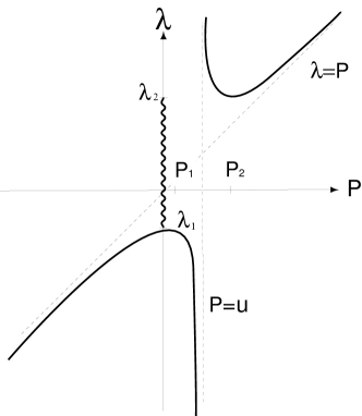
Figure 5: The $g=0$ algebraic curve (3.8).

Note that the spectral of $L$ is given by Spec$(L)=(-\infty,{\lambda}_{1}]\cup[{\lambda}_{2},\infty)$. The $g=0$ Riemann surface has a topology of a sphere as shown in Fig.6. Thus the hyperbolic system (2.7) can be considered as an approximate system of the NLS equation on the $g=0$ Riemann surface.

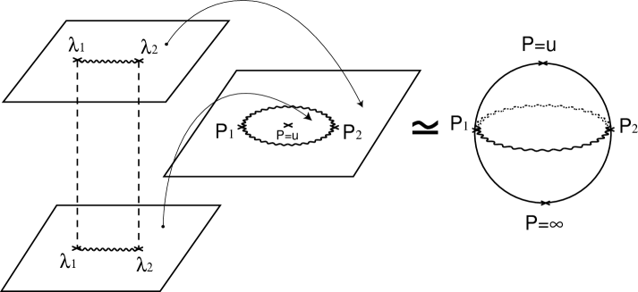
Figure 6: The $g=0$ Riemann surface corresponding to the curve (3.8).

Let us first demonstrate that the system (2.7) or (3.10) can be interpreted as a dynamics of the Riemann surface of genus 0. On the $g=0$ Riemann surface, we define the following meromorphic (Abelian) differentials ${\omega}_{1}$ and ${\omega}_{2}$ of the second kind,

$${\omega}_{1}={1\over 2}\left(1+{{{\lambda}-{1\over 2}{\sigma}_{1}}\over{\sqrt{R_{0}}}}\right)d{\lambda}\sim d\lambda+O\left(\frac{d\lambda}{\lambda^{2}}\right),$$ (3.18)

$${\omega}_{2}={1\over 2}\left({\lambda}+{{{\lambda}^{2}-{1\over 2}{\sigma}_{1}{\lambda}+{1\over 2}{\sigma}_{2}-{1\over 8}{\sigma}_{1}^{2}}\over{\sqrt{R_{0}}}}\right)d{\lambda}$$

$$~{}~{}~{}~{}~{}\sim\lambda d\lambda+O\left(\frac{d\lambda}{\lambda^{2}}\right),$$ (3.19)

where ${\sigma}_{1}={\lambda}_{1}+{\lambda}_{2}(=2u)$ and ${\sigma}_{2}={\lambda}_{1}{\lambda}_{2}$. Note from Eq.(3.17) that these differentials are given by $\omega_{1}=dQ_{1}=dP$ and $\omega_{2}=dQ_{2}=PdP$, that is, $Q_{1}$ and $Q_{2}$ are the Abelian integrals. In the case of $g=0$, these differentials are trivial (image of the derivation), and it corresponds to that the fundamental group for $g=0$ surface consists of only identity, i.e. for any cycle $a$ on the surface,

$$\oint_{a}\omega_{i}=0.$$ (3.20)

Thus we have:

Proposition 3.1

The quasi-linear hyperbolic system (2.7) can be written by

$${{{\partial}{\omega}_{1}}\over{{\partial}Z}}={{{\partial}{\omega}_{2}}\over{{\partial}T}},$$ (3.21)

where $\omega_{1}$ and $\omega_{2}$ are the Abelian differentials (3.18) and (3.19) defined on the $g=0$ Riemann surface.

Equation (3.21) then defines the ($g=0$) Whitham equation [6, 18]. The differentials $\omega_{1}$ and $\omega_{2}$ in Eq.(3.21) are also given by the limits,

$$\omega_{1}=dQ_{1}=d\left(\lim_{\beta\to 0}\frac{1}{\phi}D\phi\right),$$ (3.22)

$$\omega_{2}=dQ_{2}=d\left(\lim_{\beta\to 0}\frac{1}{\phi}B_{2}\phi\right).$$ (3.23)

Thus Eq.(3.21) is just the compatibility condition of the $T$- and $Z$-flows, that is, $\partial^{2}\ln\phi/\partial T\partial Z=\partial^{2}\ln\phi/\partial Z\partial T$. Calculating the residue of (3.21) at each branch point ${\lambda}_{k}$, we obtain the Riemann invariant form of (3.21),

$${{{\partial}{\lambda}_{k}}\over{{\partial}Z}}=s_{k}({\lambda}_{1},{\lambda}_{2}){{{\partial}{\lambda}_{k}}\over{{\partial}T}},~{}~{}~{}~{}~{}k=1,2,$$ (3.24)

where the characteristic velocity $s_{k}({\lambda}_{1},{\lambda}_{2})$ is given by

$$s_{k}=\frac{{\lambda}^{2}-{1\over 2}\sigma_{1}{\lambda}+{1\over 2}\sigma_{2}-{1\over 8}\sigma_{1}^{2}}{{\lambda}-{1\over 2}\sigma_{1}}\Bigg{|}_{{\lambda}={\lambda}_{k}}.$$ (3.25)

Equation (3.24) is of course the same as (2.11). Then we can rephrase the Proposition 2.1 as:

Theorem 3.1

The $g=0$ Whitham equation (3.24) with the initial data (2.12) has a unique global solution (rarefaction wave).

We now present the NLS-Whitham equations for arbitrary genus. The two sheeted Riemann surface of genus $g$ is defined by the algebraic (hyper-elliptic) curve $y^{2}=R_{g}(\lambda)$ with

$$R_{g}({\lambda})=\prod_{k=1}^{2g+2}({\lambda}-{\lambda}_{k}),$$ (3.26)

where the branch points ${\lambda}_{k}$ are real and are assumed to satisfy ${\lambda}_{1}<{\lambda}_{2}<\ldots<{\lambda}_{2g+2}$. The Riemann surface of genus $g$ has a topology of a sphere with $g$ handles. In Fig.7, we plot the curve of $g=1$. Comparing the case with $g=0$, we see that the closed curve in the middle of the graph indicates an opening of the genus.

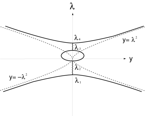
Figure 7: The $g=1$ algebraic curve $y^{2}=R_{g}({\lambda})$ in (3.26).

The NLS-Whitham equation on the genus $g$ Riemann surface is derived from the NLS equation as the slow modulation of quasi-periodic wavetrain where the spectral of the Lax operator $L$ is given by,

$$\mbox{Spec}(L)={\bf R}\backslash\{\bigcup_{i=0}^{g}({\lambda}_{2i+1},{\lambda}_{2i+2})\}.$$ (3.27)

Here we reformulate the result in [7] as an extension of the $g=0$ NLS-Whitham equation (3.21). In the case of arbitrary genus $g$, the equivalent of the Abelian differentials $\omega_{1}$ and $\omega_{2}$ defined before are given by

$${\omega}_{1}={1\over 2}\left(1+{{{\lambda}^{g+1}-{1\over 2}{\sigma}_{1}{\lambda}^{g}+\alpha_{1}\lambda^{g-1}+\cdots+\alpha_{g}}\over{\sqrt{R_{g}}}}\right)d{\lambda}$$

$$~{}~{}~{}~{}~{}~{}\sim d{\lambda}+O\left(\frac{d{\lambda}}{{\lambda}^{2}}\right),\ \mbox{as}\ \ {\lambda}\to\infty,$$ (3.28)

$${\omega}_{2}={1\over 2}\left({\lambda}+{{{\lambda}^{g+2}-{1\over 2}{\sigma}_{1}{\lambda}^{g+1}+({1\over 2}\sigma_{2}-{1\over 8}{\sigma}_{1}^{2}){\lambda}^{g}+\beta_{1}\lambda^{g-1}+\cdots+\beta_{g}}\over{\sqrt{R_{g}}}}\right)d{\lambda}$$

$$~{}~{}~{}~{}~{}~{}\sim{\lambda}d{\lambda}+O\left(\frac{d{\lambda}}{{\lambda}^{2}}\right),\ \mbox{as}\ \ {\lambda}\to\infty,$$ (3.29)

where $\sigma_{1}$, $\sigma_{2}$ (and $\sigma_{3}$) are defined by

$${\sigma}_{1}=\sum_{i=1}^{4}{\lambda}_{i},\ \ {\sigma}_{2}=\sum_{i<j}{\lambda}_{i}{\lambda}_{j},\ \ \sigma_{3}=\sum_{i<j<k}{\lambda}_{i}{\lambda}_{j}{\lambda}_{k}.$$ (3.30)

The coefficients $\alpha_{n}$ and $\beta_{n}$ in (3.28) and (3.29) are determined by the normalizations on $\omega_{1}$ and $\omega_{2}$,

$$\oint_{a_{i}}{\omega}_{1}=\oint_{a_{i}}{\omega}_{2}=0,\ \ \mbox{for}\ \ i=1,\cdots,g,$$ (3.31)

with the canonical $a_{i}$-cycle over the region $[{\lambda}_{2i+1},{\lambda}_{2i}]$. Fig.reff3:1 shows the spectral of $L$ and the canonical cycles.

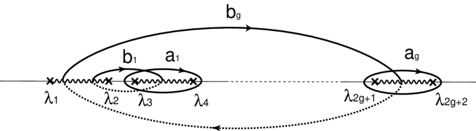
Figure 8: The 2-sheeted Riemann surface with branch cuts and canonical cycles.

Namely, we have the following $2g$ linear system of equations for $\alpha_{i}$ and $\beta_{i}$ for $i=1,\cdots,g$,

$$\left\{\begin{array}[]{ll}&\displaystyle{I_{i}^{g+1}-\frac{1}{2}\sigma_{1}I_{i}^{g}+\alpha_{1}I_{i}^{g-1}+\cdots+\alpha_{g}I^{0}_{i}=0},\\ &\displaystyle{I_{i}^{g+2}-\frac{1}{2}\sigma_{1}I_{i}^{g+1}+\left(\frac{1}{2}\sigma_{2}-\frac{1}{8}\sigma_{1}^{2}\right)I_{i}^{g}+\beta_{1}I_{i}^{g-1}+\cdots+\beta_{g}I_{i}^{0}=0},\end{array}\right.$$ (3.34)

where the integrals $I_{i}^{n}$ are given by

$$I_{i}^{n}=\frac{1}{2}\int_{{\lambda}_{2i+1}}^{{\lambda}_{2i+2}}\frac{{\lambda}^{n}}{\sqrt{-R_{g}}}d{\lambda}.$$ (3.35)

Then the NLS-Whitham equation of genus $g$ is defined by the same form as Eq.(3.21). As shown in [7, 18, 4], the Whitham equation describes the conservation laws averaged over the high oscillations appearing as a dispersive shock. Then one can introduce the fast and slow variables to describe the oscillation and the averaged behavior on the solution of the NLS equation in the weak dispersion limit [25, 6]. The average is then taken over the fast variable so that the averaged equation describes the solution behaviour in the slow scale. Thus the average is given by

$$\langle f\rangle=\langle f\rangle(T_{slow}):=\lim_{\beta\to 0}\frac{\beta}{2\pi}\int_{-\frac{\pi}{\beta}}^{\frac{\pi}{\beta}}f(T_{slow},T_{fast})dT_{fast},$$ (3.36)

where $T_{slow}$ and $T_{fast}$ are the slow and fast variables, and we use $T$ as the slow variable in the NLS-Whitham equation. Note that the rescaling $Z\to Z/\beta$ used to derive the Whitham equation (3.10) defines the slow variable $Z=Z_{slow}$, i.e. $Z_{slow}=\beta Z_{fast}$. Then the Abelian differentials $\omega_{1}$ and $\omega_{2}$ in the Whitham equation (3.21) are defined by the averages [4],

$$\omega_{1}=d\Big{\langle}-i\beta\frac{\partial}{\partial T}\ln\phi\Big{\rangle}\sim\left(1+\sum_{n=1}^{\infty}\frac{nF_{n}}{{\lambda}^{n+1}}\right)d{\lambda},$$ (3.37)

$$\omega_{2}=d\Big{\langle}-i\beta\frac{\partial}{\partial Z}\ln\phi\Big{\rangle}\sim\left({\lambda}+\sum_{n=1}^{\infty}\frac{nG_{n}}{{\lambda}^{n+1}}\right)d{\lambda}.$$ (3.38)

The Whitham equation leads to the conservation laws,

$${\partial F_{n}\over\partial Z}={\partial G_{n}\over\partial T}$$ (3.39)

in which the cases for $n=1$ and $n=2$ correspond to the averages of (2.2) and (2.3). Here $F_{n}$ and $G_{n}$ are the averaged conserved densities and fluxies, and we have for example

$$F_{1}=\left<\rho\right>=-{1\over 4}\sigma_{2}+{1\over 16}\sigma_{1}^{2}+{1\over 2}\alpha_{1},$$ (3.40)

$$F_{2}=G_{1}=\langle\rho u\rangle=\frac{1}{4}\sigma_{3}-\frac{1}{8}\sigma_{1}\sigma_{2}+\frac{1}{32}\sigma_{1}^{3}+\frac{1}{2}\beta_{1}$$

$$~{}~{}~{}~{}~{}~{}~{}~{}~{}~{}~{}~{}~{}~{}~{}~{}~{}~{}~{}~{}~{}=\frac{1}{8}\sigma_{3}-\frac{1}{8}\sigma_{1}\sigma_{2}+\frac{1}{32}\sigma_{1}^{3}+\frac{1}{8}\sigma_{1}\alpha_{1}+\frac{1}{4}\alpha_{2},$$ (3.41)

$$G_{2}=\left<\rho u^{2}+{1\over 2}\rho^{2}\right>=-{1\over 8}\sigma_{4}+{1\over 8}\sigma_{1}\sigma_{3}+{1\over 32}\sigma_{2}^{2}-{5\over 64}\sigma_{1}^{2}\sigma_{2}$$

$$~{}~{}~{}~{}~{}~{}~{}~{}~{}~{}~{}~{}~{}~{}~{}~{}~{}~{}~{}~{}~{}~{}~{}~{}~{}~{}~{}~{}+{9\over 512}\sigma_{1}^{4}+{1\over 8}\sigma_{1}\beta_{1}+{1\over 4}\beta_{2}.$$ (3.42)

One should note that the quantities $F_{n}$ are given by the averages of $D_{n}$ in (3.12), i.e. $F_{n}=\langle D_{n}\rangle$. In the particular case of $g=0$, we have $\alpha_{i}=\beta_{i}=0$, and $F_{n}$ become $P_{n}$ in (3.11), which means there is no oscillations in these quantities.

4 Control of the NRZ pulses

We now consider the initial value problem of the NLS-Whitham equation with the initial pulse having a nonzero chirp in a purpose of reducing the pulse broadening due to nonlinearity and the dispersion. The main objective is to determine the average behavior of the solution of the NLS equation (2.1) in the weak dispersion limit. In a practical situation, this describes the NRZ pulse behaviour through an optical filter which removes the high oscillations (shock) due to the initial chirp.

4.1 The hyperbolic structure of the NLS-Whitham equation

Let us first discuss the hyperbolic structure of the NLS-Whitham equation, which enables us to analyze in detail the initial value problem. As in the case of $g=0$, we have the Riemann invariant form by evaluating the residue at ${\lambda}={\lambda}_{k}$ in the NLS-Whitham equation (3.21) with $\omega_{1}$ and $\omega_{2}$ given by (3.28) and (3.29),

$$\frac{\partial{\lambda}_{k}}{\partial Z}=s_{k}({\lambda}_{1},\cdots,{\lambda}_{2g+2})\frac{\partial{\lambda}_{k}}{\partial T},\ \ \mbox{for}\ k=1,\cdots,2g+2.$$ (4.1)

where the characteristic velocities $s_{k}$ is defined by the ratio of the polynomials in $\omega_{1}$ and $\omega_{2}$, i.e.

$$s_{k}={{{\lambda}^{g+2}-{1\over 2}{\sigma}_{1}{\lambda}^{g+1}+({1\over 2}\sigma_{2}-{1\over 8}{\sigma}_{1}^{2}){\lambda}^{g}+\beta_{1}\lambda^{g-1}+\cdots+\beta_{g}}\over{{\lambda}^{g+1}-{1\over 2}{\sigma}_{1}{\lambda}^{g}+\alpha_{1}\lambda^{g-1}+\cdots+\alpha_{g}}}\Bigg{|}_{{\lambda}={\lambda}_{k}}.$$ (4.2)

Then following the ref.[19], we obtain:

Lemma 4.1

The characteristic velocities satisfy

$$i)~{}~{}~{}~{}~{}{\partial s_{k}\over\partial{\lambda}_{k}}>0,~{}~{}~{}~{}~{}~{}~{}~{}\ \mbox{for~{}}\ \ \forall k,$$ (4.3)

$$ii)~{}~{}~{}~{}~{}s_{j}>s_{k},~{}~{}~{}~{}~{}~{}~{}~{}\ \mbox{if~{}}\ \ {\lambda}_{j}>{\lambda}_{k},$$ (4.4)

Proof. Let us call the polynomials in Eq.(4.2) $\hat{P}({\lambda})$ for the denominator and $\hat{Q}({\lambda})$ for the numerator. Then from the normalizations (3.31), we have

• $\hat{P}({\lambda})$ has exactly one zero in the gap $[{\lambda}_{2i+1},{\lambda}_{2i+2}]$ for $i=0,1,\cdots,g$,

• $\hat{Q}({\lambda})$ has at least one zero in each gap.

• $s({\lambda}):=\displaystyle{\frac{\hat{Q}({\lambda})}{\hat{P}({\lambda})}\to\lambda+O\left(\frac{1}{{\lambda}}\right)}$ as ${\lambda}\to\infty$.

From these proparties, the following function can be expressed as the curve in Fig.9;

$$V_{i}({\lambda}):=s({\lambda})-s_{i}=\frac{1}{\hat{P}({\lambda})}\left(\hat{Q}({\lambda})-s_{i}\hat{P}({\lambda})\right).$$ (4.5)

It is then easy to see the relations (4.3) and (4.4).        

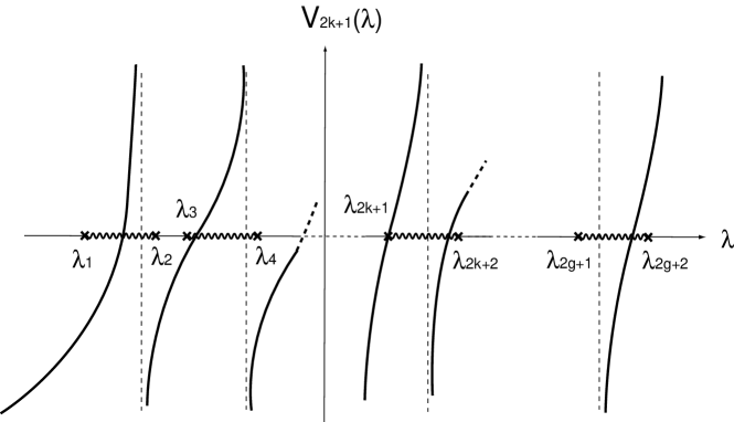
Figure 9: The function $V_{i}({\lambda})$ of (4.5) with $i=2k+1$.

From this Lemma, we have the following useful Corollary which provides a way to regularize the problem for the global existence of the solution:

Corollary 4.1

If all the initial ${\lambda}_{k}$ are monotonically decreasing and separated in the sense that for $\forall T\in{\bf R}$ and $\forall k\in\{1,2,\cdots,2g+2\}$

$$\min_{T}[{\lambda}_{k+1}(T,0)]>{\lambda}_{k}(T,0)>\max_{T}[{\lambda}_{k-1}(T,0)],$$ (4.6)

then the NLS-Whitham equation has a global solution.

4.2 Regularization of shock singularity

We now study the initial value problem of the NLS-Whitham equation with the initial data shown in Fig.10, i.e.

$$\rho(T,0)=\left\{\begin{array}[]{ll}\rho_{0},&\mbox{for~{}~{}~{} $|T|<T_{0}$}\\ 0,&\mbox{for~{}~{}~{} $|T|>T_{0}$}\end{array}\right.,$$ (4.9)

(4.10)

$$u(T,0)=\left\{\begin{array}[]{lll}-u_{0},&\mbox{for~{}~{}~{} $-T_{0}<T<0$}\\ u_{0},&\mbox{for~{}~{}~{} $0<T<T_{0}$}\\ 0,&\mbox{otherwise}\end{array}\right..$$ (4.14)

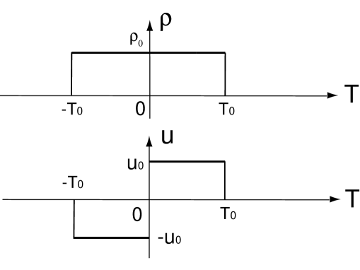
Figure 10: The initial phase modulation for one-bit NRZ pulse.

Here we vary the value of initial chirp $u_{0}$, and study its effect for a purpose of reducing the NRZ pulse broadening. As an example of real situation, we show in Fig.11 a numerical result showing the effect of initial chirp for a 16bit coded data (0010110010111100). Here the initial phase modulation is set to be periodic with the period given by the width of one-bit pulse (bit-synchronous modulation), and the output is smoothed out by using a filter (averaged over high oscillations). As seen in the Figure, the overlapping of pulses in a) with no initial phase is suppressed by the periodic initial phase modulation. The period is seen for example in (00111100) part as the elevation and depression of the pulse level. It looks that NRZ pulse with an initial phase modulation tends to deform into an RZ pulse which may have a better property in signal processing in a network system of optical communication.

Before we start to analyze this solution behaviour in detail, let us recall that the value of the $u$ corresponds to the initial velocity of the water, and the positive (negative) value of $u$ gives an compression (expansion). So we see a shock formation for the positive $u$ and a rarefaction wave for the negative $u$, which explains the pulse deformation shown in Fig.11. We also note from Eq.(3.1) that the characteristic speed for zero chirp is given by $2\sqrt{\rho}$, so that we expect to see a different behavior of the solution for each $u_{0}$ value, ($i$) $u_{0}>2\sqrt{\rho_{0}}$, ($ii$) $0<u_{0}<2\sqrt{\rho_{0}}$, ($iii$) $0>u_{0}>-2\sqrt{\rho_{0}}$, and ($iv$) $u_{0}<-2\sqrt{\rho_{0}}$. This situation is quite similar to the case of Toda lattice equation discussed in [4]. We then show that by choosing an appropriate number of genus for a given initial data and by solving the corresponding NLS-Whitham equation, one can obtain a global solution. In the form (LABEL:initialg), we here consider the case with $T_{0}=\infty$, since the edges of the pulse with constant chirp do not give any essential change from the case with zero chirp except the velocity of the expansion.

Figure 11: Effect of initial phase modulation for NRZ pulse propagation. a) Without, and b) with the initial modulation.

We now consider each of the four cases separately:

(i) The case where $u_{0}>2\sqrt{\rho_{0}}$:

In this case, the $g=0$ Riemann invariants ${\lambda}_{1}$ and ${\lambda}_{2}$ at $Z=0$ are given by increasing functions, i.e.

$${\lambda}_{1}(T,0)=\left\{\begin{array}[]{ll}-u_{0}-2\sqrt{\rho_{0}},&\mbox{for~{}~{}~{}~{} $T<0$}\\ u_{0}-2\sqrt{\rho_{0}},&\mbox{for~{}~{}~{}~{} $T>0$}\end{array}\right.,$$ (4.17)

(4.18)

$${\lambda}_{2}(T,0)=\left\{\begin{array}[]{ll}-u_{0}+2\sqrt{\rho_{0}},&\mbox{for~{}~{}~{}~{} $T<0$}\\ u_{0}+2\sqrt{\rho_{0}},&\mbox{for~{}~{}~{}~{} $T>0$}\end{array}\right..$$ (4.21)

Then we see from Corollary 4.1 that the $g=0$ NLS-Whitham equation develops a shock. So we have to use the nonzero genus NLS-Whitham equation for the regular solution. First we note:

Lemma 4.2

The initial data can be identified as the following $g=1$ data,

$${\lambda}_{1}=-u_{0}-2\sqrt{\rho_{0}},~{}~{}~{}~{}\mbox{for~{}~{} $\forall T$},$$

$${\lambda}_{2}=\left\{\begin{array}[]{ll}-u_{0}+2\sqrt{\rho_{0}},&~{}~{}~{}~{}\mbox{for~{}~{} $T<0$},\\ -u_{0}-2\sqrt{\rho_{0}},&~{}~{}~{}~{}\mbox{for~{}~{} $T>0$}.\end{array}\right.$$ (4.24)

(4.25)

$${\lambda}_{3}=\left\{\begin{array}[]{ll}u_{0}+2\sqrt{\rho_{0}},&~{}~{}~{}~{}\mbox{for~{}~{} $T<0$},\\ u_{0}-2\sqrt{\rho_{0}},&~{}~{}~{}~{}\mbox{for~{}~{} $T>0$},\end{array}\right.$$ (4.28)

$${\lambda}_{4}=u_{0}+2\sqrt{\rho_{0}},~{}~{}~{}~{}~{}\mbox{for~{}~{} $\forall T$},$$

Proof. To prove the Lemma, we need to show the values $\langle\rho\rangle$ and $\langle\rho u\rangle$ in (3.40) and (3.41) for $g=1$ become $\langle\rho\rangle=\rho$ and $\langle\rho u\rangle=\rho u$ at the point $Z=0$, that is, the initial data is a degenerate $g=1$ data. The quantities $\alpha_{1}$ and $\beta_{1}$ in (3.40) and (3.41) are determined by the normalization (3.31), that is, from (3.34)

$$\left\{\begin{array}[]{ll}&\displaystyle{I_{1}^{2}-\frac{1}{2}\sigma_{1}I_{1}^{1}+\alpha_{1}I_{1}^{0}=0},\\ &\displaystyle{I_{1}^{3}-\frac{1}{2}\sigma_{1}I_{1}^{2}+\left(\frac{1}{2}\sigma_{2}-\frac{1}{8}\sigma_{1}^{2}\right)I_{1}^{1}+\beta_{1}I_{1}^{0}=0},\end{array}\right.$$ (4.31)

with

$$I_{1}^{k}=\frac{1}{2}\int_{{\lambda}_{3}}^{{\lambda}_{4}}{{{\lambda}^{k}}\over\sqrt{-({\lambda}-{\lambda}_{1})({\lambda}-{\lambda}_{2})({\lambda}-{\lambda}_{3})({\lambda}-{\lambda}_{4})}}d{\lambda}.$$

Substituting ${\lambda}={\lambda}_{3}+({\lambda}_{4}-{\lambda}_{3})\sin^{2}\theta$ as in [4], we have a convenient form of $I^{k}_{1}$,

$$I_{1}^{k}=\int_{0}^{\pi/2}{{[{\lambda}_{3}+({\lambda}_{4}-{\lambda}_{3})\sin^{2}\theta]^{k}}\over\sqrt{[{\lambda}_{3}-{\lambda}_{1}+({\lambda}_{4}-{\lambda}_{3})\sin^{2}\theta][{\lambda}_{3}-{\lambda}_{2}+({\lambda}_{4}-{\lambda}_{3})\sin^{2}\theta]}}d\theta.$$

Now let us compute $\langle\rho\rangle$ and $\langle\rho u\rangle$. We first note that the Riemann invariants has the following symmetry in the $T$-coordinate:

$${\lambda}_{k}(-T)=-{\lambda}_{5-k}(T),\ \ \mbox{for}~{}~{}~{}k=1,\cdots,4,$$ (4.32)

so that we have

$$\begin{array}[]{lll}&\displaystyle{\sigma_{k}(-T)=(-1)^{k}\sigma_{k}(T),~{}~{}~{}~{}\mbox{for}~{}~{}~{}k=1,\cdots,4},\\ &{}\\ &\displaystyle{I_{1}^{n}(-T)=(-1)^{n}I_{1}^{n}(T),~{}~{}~{}~{}\mbox{for}~{}~{}~{}n=1,2,\cdots}.\end{array}$$ (4.36)

Thus we consider only the case with $T<0$. We then have $I_{1}^{k}={\lambda}_{3}^{k}I_{1}^{0}$ and $\alpha_{1}=-u_{0}(u_{0}+2\sqrt{\rho_{0}}),\beta_{1}=2\rho_{0}(u_{0}+2\sqrt{\rho_{0}})$, indicating that we do have $g=1$ initial data. Using these values, it is straightforward to show the result $\langle\rho\rangle=\rho_{0}$ and $\langle\rho u\rangle=-\rho_{0}u_{0}$ for $T<0$.        

The point here is to recognize that the initial data is degenerate and can also be identified as a non-zero genus data in which the Riemann invariants are decreasing functions of $T$. Then we have:

Theorem 4.1

For $u_{0}>2\sqrt{\rho_{0}}$, the $g=1$ NLS-Whitham equation with the initial data (LABEL:initiali) has a global solution.

Proof. First note that ${\lambda}_{k}=$constant remains for $\forall Z$. So we only need to determine the evolutions for ${\lambda}_{2}$ and ${\lambda}_{3}$. In order to compute these values, we first regularize them at $T=0$: From the relation (4.4) in Corollary 4.1, we have $s_{2}(T)<s_{3}(T)$ for $\forall T$, in particular, $s_{2}^{-}(0)<s_{3}^{-}(0)$ and $s_{2}^{+}(0)<s_{3}^{+}(0)$, where $s_{k}^{\pm}(0):=\lim_{\epsilon\to 0\pm}s_{k}(\epsilon)$. So if we impose

$${\lambda}_{2}(T)\equiv\lim_{\epsilon\to 0+}{\lambda}_{1}(T-\epsilon),\ \ \ \mbox{and}\ \ \ {\lambda}_{3}(T)\equiv\lim_{\epsilon\to 0-}{\lambda}_{4}(T-\epsilon),$$ (4.37)

then we have $s_{3}^{+}>s_{2}^{-}$, and therefore from (4.3) in Corollary 4.1 we obtain the global solutions for ${\lambda}_{2}$ and ${\lambda}_{3}$. We confirm this by caluculating explicitely the evolution of the Riemann invariants. The formula of $s_{k}:=s({\lambda})|_{{\lambda}={\lambda}_{k}}$ for the $g=1$ case is given by

$$s({\lambda})={{{\lambda}^{3}-{1\over 2}{\sigma}_{1}{\lambda}^{2}+({1\over 2}{\sigma}_{2}-{1\over 8}{\sigma}_{1}^{2}){\lambda}+\beta_{1}}\over{{\lambda}^{2}-{1\over 2}{\sigma}_{1}{\lambda}+\alpha_{1}}},$$ (4.38)

Using (4.31), this can be written by

$$s({\lambda})=-\frac{1}{2}\sigma_{1}+{{{\lambda}^{3}-{I_{1}^{3}\over I_{1}^{0}}+({1\over 2}{\sigma}_{2}-{3\over 8}{\sigma}_{1}^{2})({\lambda}-{I_{1}^{1}\over I_{1}^{0}})}\over{{\lambda}^{2}-{I_{1}^{2}\over I_{1}^{0}}-{1\over 2}{\sigma}_{1}({\lambda}-{I_{1}^{1}\over I_{1}^{0}})}}$$ (4.39)

We now compute $s^{-}_{3}$ as well as $s^{+}_{3},s^{-}_{2}$, and $s^{+}_{2}$. However, from the symmetry discussed in the proof of Lemma 4.2, we have $s_{3}^{-}=-s_{2}^{+},s_{3}^{+}=-s_{2}^{-}$, and also $s_{3}^{-}>s_{3}^{+}$ from (4.3) in Corollary 4.1. So we need to compute only $s_{3}^{-}$ and $s_{3}^{+}$, which can be evaluated for the region of $T<0$. In the computation of $s_{3}^{-}$, we have ${\lambda}_{1}=-{\lambda}_{3}=-{\lambda}_{4}=-u_{0}-2\sqrt{\rho_{0}}$ and ${\lambda}_{2}=-u_{0}+2\sqrt{\rho_{0}}$. Then we find $I_{1}^{k}={\lambda}_{3}^{k}I_{1}^{0}$, and obtain

$$s_{3}^{-}=(u_{0}+\sqrt{\rho_{0}})\left(1+\frac{u_{0}\sqrt{\rho_{0}}}{(u_{0}+\sqrt{\rho_{0}})^{2}}\right).$$ (4.40)

In the case of $s_{3}^{+}$, we have ${\lambda}_{1}=-{\lambda}_{4}=-u_{0}-2\sqrt{\rho_{0}}$ and ${\lambda}_{2}=-{\lambda}_{3}=-u_{0}+2\sqrt{\rho_{0}}$. Then we obtain

$$s_{3}^{+}={u_{0}^{2}-6u_{0}\sqrt{\rho_{0}}+4\rho_{0}+6\sqrt{\rho_{0}}(u_{0}-2\sqrt{\rho_{0}})J_{1}+8\sqrt{\rho_{0}}J_{2}\over u_{0}-2\sqrt{\rho_{0}}(1-J_{1})}$$ (4.41)

where $J_{n},n=1,2,$ are given by

$$J_{n}=\displaystyle{\int_{0}^{\pi/2}{\sin^{2n+2}\theta d\theta\over\sqrt{(1+a^{2}\sin^{2}\theta)(1+a^{2}\cos^{2}\theta)}}\Big{/}\int_{0}^{\pi/2}{\sin^{2}\theta d\theta\over\sqrt{(1+a^{2}\sin^{2}\theta)(1+a^{2}\cos^{2}\theta)}}},$$

where $a^{2}=2\sqrt{\rho_{0}}/u_{0}<1$. One can check the relation,

$$s_{3}^{-}>s_{3}^{+}>0.$$ (4.42)

This proves that the $g=1$ NLS-Whitham equation with the initial data (LABEL:initiali) admits a global solution.        

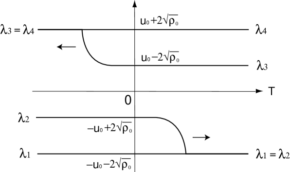
Figure 12: Evolution of the Riemann invariants for $u_{0}>2\sqrt{\rho_{0}}$.

Figure 13: Deformation of the pulse $\rho(T,Z)$ for $u_{0}>2\sqrt{\rho_{0}}$.

In Fig.12, we plot the evolution of ${\lambda}_{2}$ and ${\lambda}_{3}$ together with the constants ${\lambda}_{1}$ and ${\lambda}_{4}$. We also plot in Fig.13 the shape of the pulse $\rho(T,Z)$ at $Z=3\beta\approx 0.95$ obtained by the numerical simulation of the NLS equation (2.1) with $\rho_{0}=1,u_{0}=9\beta\approx 2.85$ and $\beta_{2}=-0.1$. We see here nearly steady oscillation in the center region $|T|<s_{3}^{+}Z$, which indicates the $g=1$ periodic solution of the NLS equation as predicted in Fig.12.

(ii) The case where $2\sqrt{\rho_{0}}>u_{0}>0$:

This case also gives a compression of the pulse, and we expect a shock formation in the system Eq.(2.7). So we again need to use the nonzero genus NLS-Whitham equation for the regularization. As in the previous case, we first identify the initial data (LABEL:initialg) as a non-zero genus data expressed as decreasing functions:

Lemma 4.3

The initial data (LABEL:initialg) with $2\sqrt{\rho_{0}}>u_{0}>0$ can be considered as a $g=2$ initial data,

$${\lambda}_{1}=-u_{0}-2\sqrt{\rho_{0}},~{}\ \mbox{for~{} $\forall T$},$$

$${\lambda}_{2}=\left\{\begin{array}[]{ll}u_{0}-2\sqrt{\rho_{0}},&\ \mbox{for}\ \ T<0,\\ -u_{0}-2\sqrt{\rho_{0}},&\ \mbox{for}\ \ T>0.\end{array}\right.$$ (4.45)

$${\lambda}_{3}=u_{0}-2\sqrt{\rho_{0}},~{}\ \mbox{for~{} $\forall T$},$$

(4.46)

$${\lambda}_{4}=-u_{0}+2\sqrt{\rho_{0}},~{}\ \mbox{for~{} $\forall T$},$$

$${\lambda}_{5}=\left\{\begin{array}[]{ll}u_{0}+2\sqrt{\rho_{0}},&\ \mbox{for}\ \ T<0,\\ -u_{0}+2\sqrt{\rho_{0}},&\ \mbox{for}\ \ T>0,\end{array}\right.$$ (4.49)

$${\lambda}_{6}=u_{0}+2\sqrt{\rho_{0}},~{}\ \mbox{for~{} $\forall T$},$$

Proof. The reflective symmetry in the data mentioned in the previous case holds here as well, and we have

$${\lambda}_{k}(-T)=-{\lambda}_{7-k}(T),~{}~{}~{}~{}\ \mbox{for ~{}~{}~{}}k=1,\cdots,6,$$ (4.50)

which lead to

$$\sigma_{k}(-T)=(-1)^{k}\sigma_{k}(T),~{}~{}~{}~{}\mbox{for}~{}~{}~{}k=1,\cdots,6.$$ (4.51)

The integrals $I_{i}^{n}$ of (3.35) with $g=2$ also satisfy

$$I_{i}^{n}(-T)=(-1)^{n}I_{i}^{n}(T),~{}~{}~{}~{}\mbox{for}~{}~{}~{}i=1,2,~{}~{}\mbox{and ~{}~{}}n=1,2,\cdots.$$ (4.52)

As in the previous case, we need to compute $\langle\rho\rangle$ and $\langle\rho u\rangle$ for only $T<0$.

From (3.34), we see for $i=0,1$

$$\displaystyle{\alpha_{i+1}=\frac{(-1)^{i+1}}{[1,0]}\left([3,i]-\frac{1}{2}\sigma_{1}[2,i]\right)},$$ (4.53)

$$\displaystyle{\beta_{i+1}=\frac{(-1)^{i+1}}{[1,0]}\left\{[4,i]-\frac{1}{2}\sigma_{1}[3,i]+\left(\frac{1}{2}\sigma_{2}-\frac{1}{8}\sigma_{1}^{2}\right)[2,i]\right\}},$$ (4.54)

where

$$[n,m]:=\det\left(\matrix{I_{1}^{n}&I_{1}^{m}\cr I_{2}^{n}&I_{2}^{m}\cr}\right).$$

For $T<0$ we note that ${\lambda}_{1}=-{\lambda}_{5}=-{\lambda}_{6}$ and ${\lambda}_{2}={\lambda}_{3}=-{\lambda}_{4}$. Then caluculating $[n,m]$ leads to $\alpha_{1}=-({\lambda}_{1}^{2}+{\lambda}_{2}^{2})/2,\beta_{1}=({\lambda}_{2}-{\lambda}_{1})^{3}/8$, and using $\sigma_{1}=({\lambda}_{2}-{\lambda}_{1}),\sigma_{2}=-({\lambda}_{1}^{2}+{\lambda}_{2}^{2}+{\lambda}_{1}{\lambda}_{2}),\sigma_{3}=({\lambda}_{1}-{\lambda}_{2})({\lambda}_{1}^{2}+{\lambda}_{2}^{2})$, we verify

$$\displaystyle{\langle\rho\rangle=\frac{1}{2}({\lambda}_{1}+{\lambda}_{2})^{2}=\rho_{0}},$$ (4.55)

$$\displaystyle{\langle\rho u\rangle=\frac{1}{32}({\lambda}_{1}+{\lambda}_{2})^{2}({\lambda}_{1}-{\lambda}_{2})=-\rho_{0}u_{0}}.$$ (4.56)

This completes the proof.        

From this lemma, we obtain:

Theorem 4.2

For $2\sqrt{\rho_{0}}>u_{0}>0$, the $g=2$ NLS-Whitham equation with the initial data (LABEL:initialg2) admits the global solution.

Proof. We need to compute the velocities $s^{-}_{5}(=-s_{2}^{+})$ and $s^{+}_{5}(=-s_{2}^{-})$. The regularization of the initial data is the same as the previous case, and we here impose

$${\lambda}_{2}(T)\equiv\lim_{\epsilon\to 0+}{\lambda}_{2}(T-\epsilon),~{}~{}~{}~{}{\lambda}_{5}(T)\equiv\lim_{\epsilon\to 0-}{\lambda}_{5}(T-\epsilon).$$ (4.57)

Then calculating the integrals given by the normalizations (3.31), we obtain the follwing results,

$$\begin{array}[]{rcl}&&\displaystyle{s_{5}^{-}=-s_{2}^{+}=(u_{0}+\sqrt{\rho_{0}})\left(1+\frac{u_{0}\sqrt{\rho_{0}}}{(u_{0}+\sqrt{\rho_{0}})^{2}}\right)},\\ &&\displaystyle{s_{5}^{+}=-s_{2}^{-}=-\frac{1}{2}u_{0}+\sqrt{\rho_{0}}}>0.\end{array}$$ (4.58)

(We omit the details of the calculation, since the procedure is the same as in [4] and is straightforward but so tedious.) This confirms the existence of the global solution.        

The solution $\langle\rho\rangle$ can be caluculated from (3.40), and in the region $|T|<s_{5}^{+}Z$, it takes the constant value,

$$\langle\rho\rangle=\rho_{0}\left(1+\frac{u_{0}}{2\sqrt{\rho_{0}}}\right)^{2}>\rho_{0}.$$ (4.59)

This explains the elevation of the pulse level observed in Fig.11. In Fig.14, we plot the evolution of the Riemann invariants. The corresponding solution $\rho(T,Z)$ at $Z=5\beta\approx 1.58$ of the numerical simulation of the NLS equation (2.1) is shown in Fig.4, where $\rho_{0}=1,u_{0}=3\beta\approx 0.95$ with $\beta_{2}=-0.1$. Note in Fig.4 that the non-oscillating part with the constant level (4.59) in the center region $|T|<s_{5}^{+}Z$ corresponds to the $g=2$ (degenerated into $g=0$) solution, and the oscillating parts in the regions $s_{5}^{+}Z<|T|<s_{5}^{-}Z$ to the ones (degenertated into $g=1$), as predicted in Fig.14. One should compare Fig.4 with Fig.13 to see the difference in the center regions.

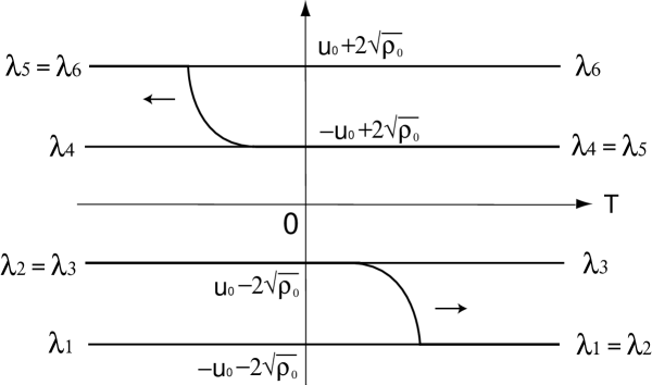
Figure 14: Evolution of the Riemann invariants for $0<u_{0}<2\sqrt{\rho_{0}}$.

(iii) The case with $0>u_{0}>-2\sqrt{\rho_{0}}$:

In this case, the initial data gives decreasing functions for both ${\lambda}_{1}$ and ${\lambda}_{2}$ (see Fig.2), and we have:

Theorem 4.3

For $0>u_{0}>-2\sqrt{\rho_{0}}$, the $g=0$ NLS-Whitham equation admits the global solution with the initial data (LABEL:initialg).

Proof. In this case, ${\lambda}_{1}$ and ${\lambda}_{2}$ can be regularized as

$${\lambda}_{1}(T)\equiv\lim_{\epsilon\to 0+}{\lambda}_{1}(T-\epsilon),\ \ \ \mbox{and}\ \ \ {\lambda}_{2}(T)\equiv\lim_{\epsilon\to 0-}{\lambda}_{2}(T-\epsilon).$$ (4.60)

Then from Eq.(4.2) of $s_{k}$ for $g=0$, we obtain

$$\begin{array}[]{rcl}&&\displaystyle{s_{2}^{-}=-s_{1}^{+}=-u_{0}+\sqrt{\rho_{0}}>0},\\ &&\displaystyle{s_{2}^{+}=-s_{1}^{-}=\frac{1}{2}(u_{0}+2\sqrt{\rho_{0}})>0}.\end{array}$$ (4.61)

Thus we have $s_{2}^{-}>s_{2}^{+}>0>s_{1}^{-}>s_{1}^{+}$, which implies the assertion of the theorem.        

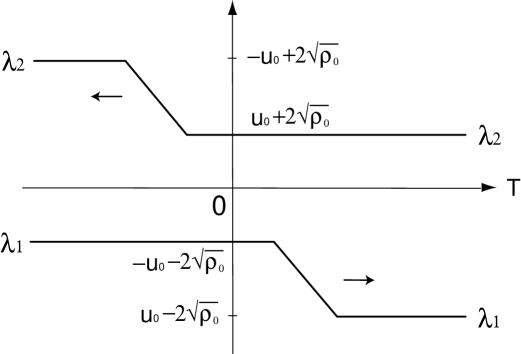
Figure 15: Evolution of the Riemann invariants for $0>u_{0}>-2\sqrt{\rho_{0}}$.

Figure 16: Deformation of the pulse $\rho(T,Z)$ for $0>u_{0}>-2\sqrt{\rho_{0}}$: Solid curve, the numerical result; Dashed curve, the solution of Eq.(4.67).

We also find the solutions ${\lambda}_{1},{\lambda}_{2}$ and $\langle\rho(T,Z)\rangle=\rho(T,Z)$: For $T>0$,

$${\lambda}_{1}(T,Z)=\left\{\begin{array}[]{lll}\displaystyle{u_{0}-2\sqrt{\rho_{0}}},&\mbox{for~{}~{}~{} $T>s_{2}^{-}Z$},\\ \displaystyle{-\frac{4}{3Z}T-\frac{1}{3}(u_{0}+2\sqrt{\rho_{0}})},&\mbox{for~{} $s_{2}^{+}Z<T<s_{2}^{-}Z$},\\ \displaystyle{-u_{0}-2\sqrt{\rho_{0}}},&\mbox{for~{}~{}~{} $0<T<s_{2}^{+}Z$},\end{array}\right.$$ (4.65)

(4.66)

$${\lambda}_{2}(T,Z)=u_{0}+2\sqrt{\rho_{0}},~{}~{}~{}~{}~{}~{}\mbox{for~{}~{}~{} $\forall T>0$,}$$

and

$$\rho(T,Z)=\left\{\begin{array}[]{lll}\displaystyle{{\rho_{0}}},&\mbox{for~{}~{}~{} $T>s_{2}^{-}Z$},\\ \displaystyle{\frac{1}{9Z^{2}}\left\{T+(u_{0}+2\sqrt{\rho_{0}})Z\right\}^{2}},&\mbox{for~{}~{} $s_{2}^{+}Z<T<s_{2}^{-}Z$},\\ \displaystyle{\rho_{0}\left(1+\frac{u_{0}}{2\sqrt{\rho_{0}}}\right)^{2}},&\mbox{for~{}~{}~{} $0<T<s_{2}^{+}Z$},\end{array}\right.$$ (4.67)

For $T<0$, note the symmetry ${\lambda}_{1}(-T,Z)=-{\lambda}_{2}(T,Z)$ and $\rho(-T,Z)=\rho(T,Z)$. These solutions are shown in Fig.15 and Fig.16. In Fig.16, we also plot the numerical result $\rho(T,Z)$ at $Z=10\beta\approx 3.16$ of the NLS equation (2.1) where $\rho_{0}=1,u_{0}=-3\beta\approx-0.95,\beta_{2}=-0.1$, which agrees quite well with the analytical solution (4.67). Note that the level of $\rho$ for $|T|<s_{2}^{+}Z$ has the same formula as the previous case except the sign of $u_{0}$. This explains the bit-wise depression in the pulse level shown in Fig.11, and it leads to the deformation into a RZ-like pulse observed in the experiment [3]. This also gives a theoretical limit of the strength of the initial chirp, i.e. $u_{0}>-2\sqrt{\rho_{0}}$, to avoid a destruction of the pulse. In fact, we will see below that the case with $u_{0}<-2\sqrt{\rho_{0}}$ the level of the signal becomes zero starting from $T=0$, the point of the discontinuity in chirp.

(iv) The case where $u_{0}<-2\sqrt{\rho_{0}}$:

We first have:

Lemma 4.4

The initial data (LABEL:initialg) for $u_{0}<-2\sqrt{\rho_{0}}$ can be considered as a $g=1$ initial data where the Riemann invariants ${\lambda}_{1},\cdots,{\lambda}_{4}$ have the following values,

$${\lambda}_{1}=\left\{\begin{array}[]{ll}u_{0}+2\sqrt{\rho_{0}},&\mbox{for~{}~{} $T<0$,}\\ u_{0}-2\sqrt{\rho_{0}},&\mbox{for~{}~{} $T>0$,}\end{array}\right.$$ (4.70)

$${\lambda}_{2}=u_{0}+2\sqrt{\rho_{0}},~{}~{}\mbox{for~{}~{}$\forall T$,}$$

(4.71)

$${\lambda}_{3}=-u_{0}-2\sqrt{\rho_{0}},~{}~{}\mbox{for~{}~{}$\forall T$,}$$

$${\lambda}_{4}=\left\{\begin{array}[]{ll}-u_{0}+2\sqrt{\rho_{0}},&\mbox{for~{}~{} $T<0$,}\\ -u_{0}-2\sqrt{\rho_{0}},&\mbox{for~{}~{} $T>0$.}\end{array}\right.$$ (4.74)

Proof. The calculation to show $\langle\rho\rangle=\rho$ and $\langle\rho u\rangle=\rho u$ is the same as the previous cases, and we omit it.        

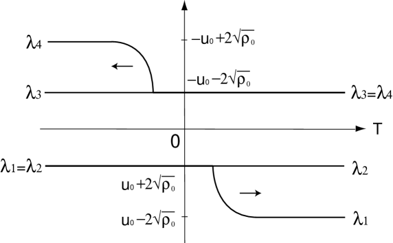
Figure 17: Evolution of the Riemann invariants for $u_{0}<-2\sqrt{\rho_{0}}$.

In Fig.17, we plot the initial data as the solid lines. Since all the Riemann invariants ${\lambda}_{k}$ satisfy the conditions in Corollary 4.1, we obtain:

Theorem 4.4

For $u_{0}<-2\sqrt{\rho_{0}}$, the $g=1$ NLS-Whitham equation with the initial data (LABEL:initialiv) has a global solution.

Proof. We determine the evolutions for ${\lambda}_{1}$ and ${\lambda}_{4}$. The regularization of ${\lambda}_{1}$ and ${\lambda}_{4}$ at $T=0$ is given by imposing

$${\lambda}_{1}(T)\equiv\lim_{\epsilon\to 0+}{\lambda}_{1}(T-\epsilon),\ \ \ \mbox{and}\ \ \ {\lambda}_{4}(T)\equiv\lim_{\epsilon\to 0-}{\lambda}_{4}(T-\epsilon).$$ (4.75)

Then we have $s_{4}^{+}>s_{1}^{-}$, and therefore we obtain the global solution as in the previous cases. In fact, from the formula of $s_{k}$, we have

$$\begin{array}[]{rcl}&&\displaystyle{s_{4}^{-}=-s_{1}^{+}=-u_{0}+\sqrt{\rho_{0}}>0},\\ &&{}\\ &&\displaystyle{s_{4}^{+}=-s_{1}^{-}=-u_{0}-2\sqrt{\rho_{0}}>0}.\end{array}$$ (4.76)

This completes the proof.        

We note in particular that the solution $\langle\rho(T,Z)\rangle$ in the center region $|T|<s_{4}^{+}Z$ becomes zero, which is obtained from Eq.(3.40) with $\sigma_{1}=0,\sigma_{2}=-2{\lambda}_{3}^{2},I_{1}^{k}={\lambda}_{3}^{k}I_{1}^{0}$ and $\alpha_{1}=-{\lambda}_{3}^{2}$. In Fig.18, we plot the pulse profile $\rho(T,Z)$ at $Z=3\beta\approx 0.95$ obtained by the numerical simulation of the NLS equation (2.1) with $\rho_{0}=1,u_{0}=-9\beta\approx-2.85$ and $\beta_{2}=-0.1$. As was predicted by the theory, the pulse level at $T=0$ becomes zero right after the propagation. One should also note that the genus is actually degenerated into $g=0$ for $\forall T$, even though we need the $g=1$ regularized initial data for the global solution. This implies that the solution is indeed $g=1$, but there is no oscillations in the solution. The small oscillations observed in Fig.18 are due to a nonzero value of $\beta_{2}$, and disappear in the limit $\beta_{2}\to 0$.

Figure 18: Deformation of the pulse $\rho(T,Z)$ for $u_{0}<-2\sqrt{\rho_{0}}$.

In this Section, we have considered the evolution of the Riemann invariants for $Z>0$ in the cases with several different values of initial chirp $u_{0}$. We then recognized that some of the cases gave degenerate genus initial data, and choosing appropriate genus, we found the global solutions for the corresponding NLS-Whitham equations. We also note that the original system of equations (2.2) and (2.3) is invariant under the change of variables $Z\to-Z$ and $u\to-u$. Hence for example the evolution of the case ($ii$) for $Z>0$ can be extended to the evolution for $Z<0$ with the case ($iii$) under the change $Z\to-Z$ and $u_{0}\to-u_{0}$. Thus we have described a change of genus along the $Z$-axis, and in the example we see the Riemann surface of $g=0$ for $Z<0$ and of $g=2$ (degenerated into $g=1$) for $Z>0$. This process is illustrated in Fig.19.

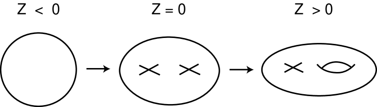
Figure 19: Deformation of the Riemann surface for $0<u_{0}<2\sqrt{\rho_{0}}$.

5 Effects of the higher order dispersion

As shown in [11, 12], the important higher order effects in a long-distance and high-speed optical communication system are described by the perturbed NLS equation,

$$i{\partial q\over\partial Z}+{\beta_{2}\over 2}{\partial^{2}q\over\partial T^{2}}+|q|^{2}q=i{\beta_{3}\over 6}{\partial^{3}q\over\partial T^{3}}+i\gamma{\partial\over\partial T}(|q|^{2}q)+\sigma_{R}q{\partial\over\partial T}|q|^{2},$$ (5.1)

where $\beta_{3},\gamma,\sigma_{R}$ are real constants describing the third order linear dispersion, nonlinear dispersion due to the delay effect of the Kerr nonlinearity and the Raman (dissipative) effect. Since the NRZ system operates in a small GVD ($\beta_{2}$) regime, the third order dispersion ($\beta_{3}$) becomes particularly important. Also the Raman term may not be so important in the regime of pulsewidth with scores of pico-second. So we consider the effects of $\beta_{3}$ and $\gamma$ in Eq.(5.1). In a real system, we also use a region where $\beta_{3}$ becomes (or make) so small, and assume that $\beta_{3}\propto(\beta_{2})^{3/2}$. Then as shown in [11] Eq.(5.1) with $\sigma_{R}=0$ can be Lie-transformed to an integrable system (the NLS + its hierarchy),

$$i{\partial q\over\partial Z}+{\beta_{2}\over 2}{\partial^{2}q\over\partial T^{2}}+|q|^{2}q=i{\beta_{3}\over 6}{\partial^{3}q\over\partial T^{3}}+i{\beta_{3}\over\beta_{2}}|q|^{2}{\partial q\over\partial T}+(\mbox{higher~{}orders}).$$ (5.2)

In a small $\beta_{2}$, the transformation is however valid only for a weak nonlinear case, e.g. $|q|^{2}\sim O(\beta_{2})$. Equation (5.2) without the higher orders has also infinite number of conservation laws with the same conserved densities as the case of the NLS equation. In fact, this can be also written in the Lax form,

$$-i{\partial L\over\partial Z}=[B,L],\ \ \mbox{with}\ \ B=B_{2}+\hat{\beta}B_{3},$$ (5.3)

where $B_{n}$ are defined in (3.4), and $\hat{\beta}=-\beta_{3}/(2\beta^{3})$ with $\beta_{2}\equiv-\beta^{2}$. The explicit formula of $B_{3}$ is given by

$$B_{3}=\frac{1}{3}D^{3}+\rho D+\rho u+\frac{1}{2}D\rho.$$ (5.4)

Now let us take the limit $\beta\to 0$, and assume both $\rho$ and $u$ are smooth. Then as in the previous section we have the $g=0$ approximation of the equation (5.2), which is obtained in the form similar to (3.10) with the rescaling $Z\to Z/\beta$,

$${\partial Q_{1}\over\partial Z}={\partial\over\partial T}(Q_{2}+\hat{\beta}Q_{3}),$$ (5.5)

where $Q_{3}=[{\lambda}^{3}]_{\geq 0}=P^{3}/3+\rho P+\rho u$. In terms of $\rho$ and $u$, Eq.(5.5) gives a system,

$${{\partial}\over{{\partial}Z}}\left(\matrix{\rho\cr u\cr}\right) = \left(\matrix{u+\hat{\beta}(u^{2}+2\rho)&\rho+\hat{\beta}(2u\rho)\cr 1+\hat{\beta}(2u)&u+\hat{\beta}(u^{2}+2\rho)\cr}\right){{\partial}\over{{\partial}T}}\left(\matrix{\rho\cr u\cr}\right).$$ (5.6)

Since the Lax operator for the equation (5.2) is the same as the NLS case, the spectral curve in this limit is given by (3.8), and the system (5.6) is also referred as the $g=0$ Whitham equation. The eigenvalues of the coefficient matrix of (5.6) are then given by

$$s_{1,2}=u+\hat{\beta}(u^{2}+2\rho)\mp(1+2\hat{\beta}u)\sqrt{\rho}$$ (5.7)

which give the characteristic velocities of the Riemann invariants ${\lambda}_{1}$ and ${\lambda}_{2}$ in (2.12), i.e. ${\lambda}_{1,2}=u\mp 2\sqrt{\rho}$. In terms of the Riemann invariants, Eqs.(5.7) are expressed as

$$\begin{array}[]{rcl}&&s_{1}=\displaystyle{\frac{1}{4}(3{\lambda}_{1}+{\lambda}_{2})+\frac{\hat{\beta}}{8}(5{\lambda}_{1}^{2}+{\lambda}_{2}^{2}+2{\lambda}_{1}{\lambda}_{2})},\\ &&s_{2}=\displaystyle{\frac{1}{4}({\lambda}_{1}+3{\lambda}_{2})+\frac{\hat{\beta}}{8}({\lambda}_{1}^{2}+5{\lambda}_{2}^{2}+2{\lambda}_{1}{\lambda}_{2})},\end{array}$$ (5.8)

Because of the nonlinear terms of ${\lambda}_{1}$ and ${\lambda}_{2}$, the characteristic velocity does not satisfy the double monotonicity in Corollary 4.1. This implies that the $g=0$ Whitham equation (5.6) develops a shock even in the case where the Riemann invariants are both decreasing functions. To demonstrate the situation, we study the initial value problem of (5.6) with the initial data given by (2.10). As in the previous section, we calculate the characteristic velocities of the pulse edges at $T=-T_{0}$ and at $T=T_{0}$ (see Fig.2).

Let us first compute the velocity near $T=T_{0}$, where the Riemann invariant ${\lambda}_{2}$ decreases from $2\sqrt{\rho_{0}}$ to $-2\sqrt{\rho_{0}}$, and ${\lambda}_{1}=-2\sqrt{\rho_{0}}$. From Eq.(5.8), $s_{2}$ near $T=T_{0}$ is given by

$$s_{2}({\lambda}_{1}=-2\sqrt{\rho_{0}},{\lambda}_{2})=\frac{5\hat{\beta}}{8}{\lambda}_{2}^{2}+\frac{1}{4}(3-2\hat{\beta}\sqrt{\rho_{0}}){\lambda}_{2}-\frac{\sqrt{\rho_{0}}}{2}(1-\hat{\beta}\sqrt{\rho_{0}}).$$ (5.9)

To avoid a shock, we require that $s_{2}$ is a monotone increasing function in ${\lambda}_{2}\in[-2\sqrt{\rho_{0}},2\sqrt{\rho_{0}}]$. This implies that for $\hat{\beta}>0$ the velocity $s_{2}$ has to take the minimum in the region ${\lambda}_{2}\leq-2\sqrt{\rho_{0}}$, and we have the relation,

$$\frac{\partial s_{2}}{\partial{\lambda}_{2}}\Big{|}_{{\lambda}_{2}=-2\sqrt{\rho_{0}}}=-3\hat{\beta}\sqrt{\rho_{0}}+\frac{3}{4}\geq 0.$$ (5.10)

Similarly, for $\hat{\beta}<0$, $s_{2}$ has to take the maximum in ${\lambda}_{2}\geq 2\sqrt{\rho_{0}}$, and

$$\frac{\partial s_{2}}{\partial{\lambda}_{2}}\Big{|}_{{\lambda}_{2}=2\sqrt{\rho_{0}}}=2\hat{\beta}\sqrt{\rho_{0}}+\frac{3}{4}\geq 0.$$ (5.11)

From these results we obtain

$$-\frac{3}{8\sqrt{\rho_{0}}}\leq\hat{\beta}\leq\frac{1}{4\sqrt{\rho_{0}}}.$$ (5.12)

To compute also the velocity $s_{1}$ near $T=-T_{0}$, we note the symmetry of the Riemann invariant form of the $g=0$ Whitham equation (5.6), that is, for the reflection $T\to-T$ the form is invariant under the change of variables ${\lambda}_{k}\to-{\lambda}_{3-k}$ for $k=1,2$ and $\hat{\beta}\to-\hat{\beta}$. Therefore we obtain the condition to avoid a shock near $T=-T_{0}$,

$$-\frac{1}{4\sqrt{\rho_{0}}}\leq\hat{\beta}\leq\frac{3}{8\sqrt{\rho_{0}}}.$$ (5.13)

Thus we have :

Proposition 5.1

The system (6.6) with the initial data (2.10) admits a global solution if the following condition is satisfied,

$$|\hat{\beta}|\equiv\Big{|}\frac{\beta_{3}}{(-\beta_{2})^{3/2}}\Big{|}\leq\frac{1}{4\sqrt{\rho_{0}}}.$$ (5.14)

This provides a condition on design parameters in the second and third order dispersions and the power level for a smooth NRZ pulse propagation.

The solution of (5.6) can be obtained as follows: Following the proof of Proposition 2.1, for example near $T=T_{0}$, we have a single equation for ${\lambda}_{2}$,

$$\frac{\partial{\lambda}_{2}}{\partial Z}=s_{2}(-2\sqrt{\rho_{0}},{\lambda}_{2})\frac{\partial{\lambda}_{2}}{\partial T},$$ (5.15)

where $s_{2}(-2\sqrt{\rho_{0}},{\lambda}_{2})$ is given by (5.9). The solution of this equation can be obtained in the hodograph form,

$$T+s_{2}(-2\sqrt{\rho_{0}},{\lambda}_{2})Z=T_{0},$$ (5.16)

from which ${\lambda}_{2}$ gives a monotone decreasing function in $T$ from ${\lambda}_{2}=2\sqrt{\rho_{0}}$ to ${\lambda}_{2}=-2\sqrt{\rho_{0}}$, if the condition (5.14) is satisfied. In Fig.20, we plot the pulse profiles $\rho(T,Z)$ at $Z=5\beta\approx 1.58$ obtained by the numerical simulation of (5.2), where we used $\beta_{2}=-0.1$ and $\beta_{3}=0.02$, giving a case of shock formation i.e. $\hat{\beta}=0.63>0.25$ with $\rho_{0}=1$. In this example, we predict the shock formation from both edges $T=\pm T_{0}$, which are due to the violation of the conditions (5.12) and (5.13).

Figure 20: Pulse profile under the effect of third order dispersion.

The asymmetric deformation of the pulse due to the third order dispersion has been observed in the experiment [24]

It is also interesting to study how one can regularize a case where the condition (5.14) is violated. For example, if $\hat{\beta}=3/(2\sqrt{\rho_{0}})$, then $s_{2}$ takes minimum at ${\lambda}_{2}=0$. So ${\lambda}_{2}$ becomes multi-valued function in $T$ for $Z>0$, which indicates a shock formation, and one needs to regularize the initial data by choosing an appropriate genus. This will be further discussed elsewhere.

6 WDM-NRZ system

In a WDM system, signal in each channel has a different carrier frequency, and the model equation of the system can be obtained by setting the electric field $q$ of the NLS equation (2.1) in the form,

$$q=\sum_{j=1}^{N}q_{j}.$$ (6.1)

Here $q_{j}$ represents the electric field in the $j$-th channel having carrier frequency, say $\Omega_{j}$. Because of the difference in the carrier frequencies, pulse in one channel has different group velocity from those of the others, and we see pulse-pulse collision between channels. As a simple but fundamental case, we consider here the 2-channel WDM system. Then substitutng (6.1) into the NLS equation (2.1), and ignoring the mismatch of the frequency in the FWM terms, we obtain the following coupled NLS equation [21],

$$\left\{\begin{array}[]{rcl}&{}\hfil&\displaystyle{i\frac{\partial q_{1}}{\partial Z}-{\beta^{2}\over 2}\frac{\partial^{2}q_{1}}{\partial T^{2}}+(|q_{1}|^{2}+\alpha|q_{2}|^{2})q_{1}=0},\\ &{}\hfil&\\ &{}\hfil&\displaystyle{i\frac{\partial q_{2}}{\partial Z}-{\beta^{2}\over 2}\frac{\partial^{2}q_{2}}{\partial T^{2}}+(|q_{2}|^{2}+\alpha|q_{1}|^{2})q_{2}=0},\end{array}\right.$$ (6.2)

where $\alpha=2$. The validity of this model has been discussed in [17] where a dispersion management technology is used to reduce the FWM and to keep a small GVD. We should also like to mention that the system (6.2) with $\alpha=1$ is integrable, and is called the Manakov equation [20].

Let us first summarize the result in [17] for the 2-channel WDM case ($\alpha=2$). The main result in [17] is that there exists a critical frequency separation $\Delta\Omega_{c}$ such that the system with the channel separation $|\Omega_{1}-\Omega_{2}|<\Delta\Omega_{c}$ leads to a hydrodynamic-type instability. It is also interesting to note that this instability appears even in the case of $\alpha=1$, and is not essential for the specific value of $\alpha$. So we study this instability based on the Manakov equation, which enables us to characterize the instability as a deformation of the branch points on the Riemann surface defined by the spectral curve of the Lax operator for the equation.

The Lax operator $L_{M}$ for the Manakov equation takes a similar form as of the NLS equation, (3.1), and is given by

$$L_{M}=D+\sqrt{\rho_{1}}(D-u_{1})^{-1}\sqrt{\rho_{1}}+\sqrt{\rho_{2}}(D-u_{2})^{-1}\sqrt{\rho_{2}},$$ (6.3)

where $\rho_{k}$ and $u_{k}$ are of course defined by

$$q_{k}(T,Z)=\sqrt{\rho_{k}(T,Z)}\exp\left(i\frac{1}{\beta}\sigma_{k}(T,Z)\right),\ \ \mbox{for}\ \ k=1,2.$$ (6.4)

As seen from this formula, the Manakov equation can be easily extended to an integrable $N$-coupled NLS equation which may correspond to a model equation of $N$-channel WDM system. Then the Manakov equation can be written in the Lax form (3.5) with $B_{2}=(L_{M}^{2})_{+}/2$, i.e.

$$-i\beta{\partial L_{M}\over\partial Z}=[B_{2},L_{M}],$$ (6.5)

where we have rescaled $Z$ to $Z/\beta$.

Now taking the limit $\beta\to 0$ and ignoring all the terms including $\beta$, we obtain a hydrodynamic-type equation,

$${{\partial}\over{{\partial}Z}}\left(\matrix{\rho_{1}\cr u_{1}\cr\rho_{2}\cr u_{2}\cr}\right)=\left(\matrix{u_{1}&\rho_{1}&0&0\cr 1&u_{1}&\alpha&0\cr 0&0&u_{2}&\rho_{2}\cr\alpha&0&1&u_{2}\cr}\right){{\partial}\over{{\partial}T}}\left(\matrix{\rho_{1}\cr u_{1}\cr\rho_{2}\cr u_{2}\cr}\right).$$ (6.6)

Note that this equation can also be derived from the original system (6.2) with arbitrary $\alpha$ by substituting (6.4) into (6.2) in the same approximation. However a system with $\alpha\neq 1$ may not be integrable and the corresponding Whitham equation may not be constructed in a systematic manner.

To see the hyperbolicity of (6.6), we first calculate the characteristic polynomial of the coefficient matrix in (6.6),

$$[(u_{1}-s)^{2}-\rho_{1}][(u_{2}-s)^{2}-\rho_{2}]-\alpha^{2}\rho_{1}\rho_{2}=0.$$ (6.7)

As a practical example, we set the equal intensity $\rho_{1}=\rho_{2}\equiv\rho_{0}$ and the opposite frequency shifts $u_{1}=-u_{2}\equiv u_{0}$, then we have a condition for the hyperbolicity of (6.6), that is, all the eigenvalues of the coefficient matrix are real, if the following condition is satisfied,

$$|u_{0}|>[(1+\alpha)\rho_{0}]^{1/2}.$$ (6.8)

This then gives a minimum frequency separation for 2-channel WDM system for a stable NRZ pulse propagation. The instability corresponding to the complex eigenvalues (characteristic velocity) is called hydrodynamic-type instability in [17]. Thus the instability is due to the change of type of the system (6.6) from hyperbolic to elliptic.

We now consider the geometry of the instability using the Manakov equation, and discuss the associated Whitham equation to describe a schock formation in WDM system. In the limit $\beta\to 0$, we again assume the wave function $\phi$ of $L_{M}\phi=\lambda\phi$ in the WKB form (3.7), then the spectral curve ${\lambda}={\lambda}(P)$ is given by

$${\lambda}=P+{\rho_{1}\over P-u_{1}}+{\rho_{2}\over P-u_{2}},$$ (6.9)

where $P=\partial S/\partial T$, and the evolution of $P$ is given by $\partial P/\partial Z=\partial Q_{2}/\partial T$ with $Q_{2}=(1/2)[{\lambda}^{2}]_{\geq 0}=P^{2}/2+\rho_{1}+\rho_{2}$, the limit of $B_{2}\phi/\phi$ in (6.5).

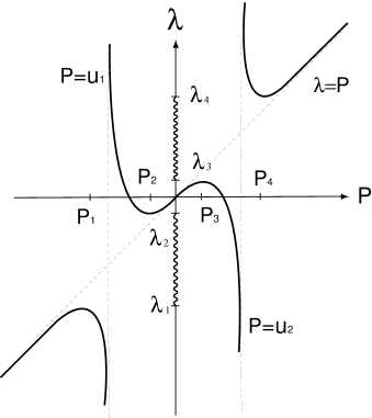
Figure 21: The $g=0$ algebraic curve (6.9).

In Fig.21, we plot the graph of Eq.(6.9) on the $P$ - ${\lambda}$ plane. As we see from Fig.21, there are at most three roots of $P$ in Eq.(6.9) for each ${\lambda}$, defining the three sheeted (non-hyperelliptic) Riemann surface. The characteristic polynomial (6.7) is then given by the equation $\partial{\lambda}/\partial P=0$, and the eigenvalues are obtained from (6.9) at the roots of this equation. Thus the spectral of $L_{M}$ of (6.3) is given by

$$\mbox{Spec}(L_{M})=(-\infty,{\lambda}_{1}]\cup[{\lambda}_{2},{\lambda}_{3}]\cup[{\lambda}_{4},\infty).$$ (6.10)

We also note that the spectral curve (6.9) defines the $g=0$ Riemann surface whose topology is a sphere obtained by a compactified $P$-plane (see Fig.22).

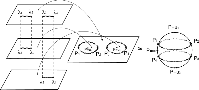
Figure 22: The $g=0$ Riemann surface corresponding to the curve (6.9).

To see these more precisely, let us study a detail of the algebraic curve (6.9). We first note Eq.(6.9) can be written as

$$4y^{3}-3\alpha_{0}({\lambda})y-\beta_{0}({\lambda})=0,$$ (6.11)

where $2y:=3P-({\lambda}+u_{1}+u_{2})$, and $\alpha_{0},\beta_{0}$ are the monic polynomials of degree 2 and 3 in ${\lambda}$,

$$\alpha_{0}=\displaystyle{{{\lambda}^{2}}-(u_{1}+u_{2}){\lambda}+u_{1}^{2}+u_{2}^{2}-u_{1}u_{2}-3(\rho_{1}+\rho_{2}),}$$ (6.12)

$$\beta_{0}=\displaystyle{{\lambda}^{3}-{3\over 2}(u_{1}+u_{2}){\lambda}^{2}-{3\over 2}\left\{u_{1}^{2}+u_{2}^{2}-4u_{1}u_{2}+3(\rho_{1}+\rho_{2})\right\}{\lambda}}$$

$$~{}~{}~{}~{}~{}~{}\displaystyle{-{9\over 2}(\rho_{1}u_{1}+\rho_{2}u_{2})+9(\rho_{1}u_{2}+\rho_{2}u_{1}).}$$ (6.13)

The roots of (6.11) are given by

$$y=\frac{1}{2}\left(\omega^{\ell}\sqrt[3]{\nu_{+}}+\omega^{3-\ell}\sqrt[3]{\nu_{-}}\right),~{}~{}~{}~{}~{}~{}~{}\mbox{for}~{}~{}~{}~{}\ell=0,1,2,$$ (6.14)

where $\omega=\exp(2\pi i/3)$, and $\nu_{\pm}$ are given by

$$\nu_{\pm}=\beta_{0}\pm\sqrt{\beta_{0}^{2}-\alpha_{0}^{3}}.$$ (6.15)

Each root lives in a different sheet, and in particular the root marked by $\ell=0$ in (6.14) lives in the fundamental sheet having the property $P\to{\lambda}$ as ${\lambda}\to\infty$. With this root, Eq.(6.6) can be identified as the $g=0$ Whitham equation in the form (3.21) where the differentials $\omega_{1}$ and $\omega_{2}$ are given by

$$\omega_{1}=dP=\frac{1}{3}\left(1+\frac{1}{3(\nu_{+})^{2/3}}{d\nu_{+}\over d{\lambda}}+\frac{1}{3(\nu_{-})^{2/3}}{d\nu_{-}\over d{\lambda}}\right)d{\lambda}$$

$$~{}~{}~{}~{}~{}~{}~{}~{}~{}~{}~{}~{}~{}\sim\left(1+\frac{\rho_{1}+\rho_{2}}{{\lambda}^{2}}+\cdots\right)d{\lambda},$$ (6.16)

$$\omega_{2}=dQ_{2}=PdP$$

$$~{}~{}~{}~{}~{}~{}~{}~{}~{}~{}~{}~{}~{}\sim\left({\lambda}+\frac{u_{1}\rho_{1}+u_{2}\rho_{2}}{{\lambda}^{2}}+\cdots\right)d{\lambda}.$$ (6.17)

The branch points (Riemann invariants) ${\lambda}_{k},k=1,\cdots,4$ are obtained from the descriminant $\Delta_{0}({\lambda})$ of the equation (6.11), that is,

$$\Delta_{0}\equiv\displaystyle{-\frac{4}{27}(\beta_{0}^{2}-\alpha_{0}^{3})}$$

$$~{}~{}~{}~{}~{}~{}=\displaystyle{(u_{1}-u_{2})^{2}\prod_{k=1}^{4}({\lambda}-{\lambda}_{k})=0}.$$ (6.18)

In the case where $u_{1}=-u_{2}\equiv u_{0}$ and $\rho_{1}=\rho_{2}\equiv\rho_{0}$, the roots of Eq.(6.18) are given by

$${\lambda}^{2}=\frac{1}{u_{0}^{2}}\left\{2u_{0}^{4}+10u_{0}^{2}\rho_{0}-\rho_{0}^{2}\pm(4u_{0}^{2}+\rho_{0})^{3/2}\sqrt{\rho_{0}}\right\}.$$ (6.19)

We also culculate the characteristic velocities $s_{k}=P_{k}\equiv P({\lambda}_{k})$ which is given by the roots of $\partial{\lambda}/\partial P=0$,

$$P^{2}=u_{0}^{2}+\rho_{0}\pm\sqrt{(4u_{0}^{2}+\rho_{0})\rho_{0}}.$$ (6.20)

If $u_{0}^{2}>2\rho_{0}$ of (6.8), these roots are all real. Note that ${\lambda}_{k}={\lambda}(P_{k})$ with the orderings ${\lambda}_{1}<{\lambda}_{2}<{\lambda}_{3}<{\lambda}_{4}$ and $P_{1}<P_{2}<P_{3}<P_{4}$. Then the condition (6.8) indicates the non-closing of the interval [${\lambda}_{2},{\lambda}_{3}$].

Now let us consider the case with nonzero genus. The corresponding algebraic curve may be given by

$$4y^{3}-3\alpha_{h}({\lambda})y-\beta_{h}({\lambda})=0,$$ (6.21)

with

$$\begin{array}[]{ll}&\alpha_{h}=\displaystyle{\prod_{j=1}^{2h+2}({\lambda}-\xi_{j}),}\\ &\beta_{h}=\displaystyle{\prod_{k=1}^{3h+3}({\lambda}-\eta_{k}),}\end{array}$$ (6.24)

where we have the relation $3\sum_{j=1}^{2h+2}\xi_{j}=2\sum_{k=1}^{3h+3}\eta_{k}$. Then the descrimenant $\Delta_{h}:=-(4/27)(\beta_{h}^{2}-\alpha_{h}^{3})$ of the curve (6.21) gives a polynomial of degree $6h+4$ in ${\lambda}$, and it indicates that there are at most $3h$ numbers of genus openning in the Whitham equation. Note that the genus of the (non-hyperelliptic) Riemann surface defined by the curve (6.21) is generically given by

$$g=3h.$$ (6.25)

The number 3 implies that gap-opening appears in between 2 sheets of the total 3 sheets. A further discussion on this subject will be given elsewhere.

Acknowledgement. The author would like to thank Ann Morlet for a useful discussion on the begining stage of this paper, and Akihiro Maruta for making several figures obtained by the numerical simulations of the NLS equation. The work is partially supported by NSF grant DMS9403597.

Figure Captions

1. Various types of a 16 bits-coded signal (0010110010111100).

2. Evolution of the Riemann invariants. Doted curve are the initial data; Solid curves are the solutions ${\lambda}_{k}(T,Z)$ for $Z>0$.

3. Deformation of NRZ pulse (Dam breaking problem). The dotted curve in $\rho$ shows the numerical result of the NLS equation.

4. Optical shock due to initial chirp.

5. The $g=0$ algebraic curve (3.8).

6. The $g=0$ Riemann surface corresponding to the curve (3.8).

7. The $g=1$ algebraic curve $y^{2}=R_{g}({\lambda})$ in (3.26).

8. The 2-sheeted Riemann surface with branch cuts and canonical cycles.

9. The function $V_{i}({\lambda})$ with $i=2k+1$.

10. The initial phase modulation for one-bit pulse.

11. Evolution of NRZ pulse with initial phase modulation. a) Without, and b) with the initial modulation.

12. Evolution of the Riemann invariants for $u_{0}>2\sqrt{\rho_{0}}$.

13. Deformation of the pulse $\rho(T,Z)$ for $u_{0}>2\sqrt{\rho_{0}}$.

14. Evolution of the Riemann invariants for $0<u_{0}<2\sqrt{\rho_{0}}$.

15. Evolution of the Riemann invariants for $0>u_{0}>-2\sqrt{\rho_{0}}$.

16. Deformation of the pulse $\rho(T,Z)$ for $0>u_{0}>-2\sqrt{\rho_{0}}$. Solid curve, the numerical result; Dashed curve, the solution (4.34).

17. Evolution of the Riemann invariants for $u_{0}<-2\sqrt{\rho_{0}}$.

18. Deformation of the pulse $\rho(T,Z)$ for $u_{0}<-2\sqrt{\rho_{0}}$.

19. Deformation of the Riemann surface for $0<u_{0}<2\sqrt{\rho_{0}}$.

20. Pulse profile under the effect of third order dispersion.

21. The $g=0$ algebraic curve (6.9).

22. The $g=0$ Riemann suface corresponding to the curve (6.9).

References

- [1] S. Aoyama, and Y. Kodama, Topological Landou-Ginzburg Theory with a Rational Potential and the Dispersionless KP Hierarchy, Comm. Math. Phys., 182 (1996) pp. 185-219.
- [2] D. J. Benney, Some prperties of long nonlinear waves, Stud. Appl. Math., 52 (1973) pp. 45-50
- [3] N. S. Bergano, C. R. Davidson, and F. Heismann, Bit-synchronous polarisation and phase modulation scheme for improving the performance of optical amplifier transmission systems, Electron. Lett. 32 (1996) pp. 52-54.
- [4] A. M. Bloch, and Y. Kodama, Dispersive regularization of the Whitham equation for the Toda lattice, SIAM J. Appl. Math. 52 (1992) pp. 909-928.
- [5] J. C. Bronski, and D. W. McLaughlin, Semiclassical behavior in the NLS equation: Optical shocks-focusing instabilities, in “Singular limits of Dispersive Waves, N. M. Ercolani, et al eds, NATO ASI Series B320 (Plenum, New York, 1994) pp. 21-38.
- [6] H. Flaschka, M. G. Forest, and D. W. McLaughlin, Multiphase averaging and the inverse spetral solution of the Korteweg-de Vries equation, Comm. Pure Appl. Math., 33 (1980), pp. 739-784.
- [7] M. G. Forest, and J.-E. Lee, Geometry and modulation theory for periodic nonlinear Schrödinger equation, in “Oscillation Theory, Computation, and Methods of Compensated Compactness”, C. Dafermos et at eds, IMA Volumes on Mathematics and Its Applications 2 (Springer-Verlag, New York, 1986) pp. 35-69.
- [8] J. Gibbons, Collisionless Boltzmann equations and integrable moment equations, Physica 3D (1981) pp. 503-511.
- [9] A. Hasegawa and Y. Kodama, Solitons in optical communications, (Oxford Univ. Press, 1995).
- [10] S. Jin, C. D. Levermore, and D. W. McLaughlin, The semiclassical limit of the defocusing NLS hierarchy (preprint).
- [11] Y. Kodama, Optical solitons in a monomode fibre, J. Stat. Phys., 39 (1985) pp. 597-614.
- [12] Y. Kodama, and A. Hasegawa, Nonlinear pulse propagation in a monomode dielectric guide, IEEE J. Quantum Electron., 23 (1987) pp. 510-524.
- [13] Y. Kodama, and J. Gibbons, Integrability of dispersionless KP hierarchy, in Proceedings of the workshop “Nonlinear World” (World Scientific, Singapore, 1990), pp. 166-180.
- [14] Y. Kodama, and S. Wabnitz, Analytical theory of guiding center NRZ and RZ signal transmission in normally dispersive nonlinear optical fibers, Opt. Lett. 20 (1995) pp. 2291-2293.
- [15] Y. Kodama, and S. Wabnitz, Compensation of NRZ signal distortion by initial frequency shifting, Electron. Lett. 31 (1995) pp. 1761-1762.
- [16] Y. Kodama, S. Wabnitz, and K. Tanaka, Control of nonreturn-to-zero signal distortion by nonlinear gain, Opt. Lett. 21 (1996) pp. 719-721.
- [17] Y. Kodama, A. Maruta, and S. Wabnitz, Minimum channel spacing in wavelength-division-multiplexed nonreturn-to-zero optical fiber transmissions, Opt. Lett. 21 (1996) pp. 1815-1817.
- [18] I. M. Krichever, Method of averaging for two-dimensional “integrable” equations, Funct. Anal. Appl., 22 (1988) pp. 37-52.
- [19] C. D. Levermore, The hyperbolic nature of the zero dispersion KdV limit, Comm. Partial Differential Equations, 13 (1988) pp. 495-514.
- [20] S. V. Manakov, On the theory of two-dimensional stationary self-focusing of electromagnetic waves, Zh. Eksp. Teor. Fiz, 65 (1974) pp. 505-516 [Sov. Phys. JETP, 38 (1974) pp. 248-253].
- [21] L. F. Mollenauer, S. G. Evangelides, and J. P. Gordon, Wavelength devision multiplexing with solitons in ultra-long distance transmission using lumped amplifiers, J. Lightwave Technol., 9 (1991) pp. 362-367.
- [22] S. Novikov, S. V. Manakov, L. P. Pitaevskii, and V. E. Zakharov, Theory of Solitons, (Plenum, New York, 1984)
- [23] M. Sato, Soliton equations as dynamical systems on an infinite dimensional Grassman manifold, RIMS Kyoto Univ. Kokyuroku 439 (1981) pp. 30-46.
- [24] H. Taga, N. Edagawa, S. Yamamoto, and S. Akiba, Recent Progress in Amplified Undersea Systems, J. Lightwave Technology, 13 (1995) pp. 829-834.
- [25] G. B. Whitham, Linear and Nonlinear Waves, (John Wiley, New York 1974).
- [26] V. E. Zakharov, and A. B. Shabat, Exact theory of two-dimensional self-focusing and one-dimensional self-modulation of waves in nonlinear media, Zh. Eksp. Teor. Fiz., 61 (1971) pp. 118-134 [Sov. Phys. JETP, 34 (1972) pp. 62-69].
- [27] V. E. Zakharov, Benney equations and quasiclassical approximation in the method of the inverse problem, Funct. Anal. Appl., 14 (1980) pp. 15-24.