We introduce a new notion of “matrix potential” to nonlinear optical systems. In terms of a matrix potential $g$, we present a gauge field theoretic formulation of the Maxwell-Bloch equation that provides a semiclassical description of the propagation of optical pulses through resonant multi-level media. We show that the Bloch part of the equation can solved identically through $g$ and the remaining Maxwell equation becomes a second order differential equation with reduced set of variables due to the gauge invariance of the system. Our formulation clarifies the (nonabelian) symmetry structure of the Maxwell-Bloch equations for various multi-level media in association with symmetric spaces $G/H$. In particular, we associate nondegenerate two-level system for self-induced transparency with $G/H=SU(2)/U(1)$ and three-level $\Lambda$- or $V$-systems with $G/H=SU(3)/U(2)$. We give a detailed analysis for the two-level case in the matrix potential formalism, and address various new properties of the system including soliton numbers, effective potential energy, gauge and discrete symmetries, modified pulse area, conserved topological and nontopological charges. The nontopological charge measures the amount of self-detuning of each pulse. Its conservation law leads to a new type of pulse stability analysis which explains nicely earlier numerical results.

1 Introduction

Since the invention of the laser, much progress has been made in understanding nonlinear interactions of radiation with matter which made nonlinear optics a fast developing and independent field of science. Recently, the interaction of laser lights with a multi-level optical medium has attracted more attention in the context of lasing without inversion [1, 2] and electromagnetically induced transparency (EIT) [3]. Laser light in general is expressed in terms of a macroscopic, classical electric field which interacts with microscopic, quantum mechanical matter. Unlike classical electrodynamics, the electric scalar potential and the magnetic vector potential do not appear to replace electromagnetic fields in nonlinear optics. Instead, the electric field itself, with appropriate restrictions to accomodate specific physical problems, plays the role of a fundamental variable which renders the problem lacking a field theoretic Lagrangian formulation. Of course, one could setup the problem in the most general QED Lagrangian framework with the conventional potential variable $A_{\mu}$, but the nonlinearity of interactions and various approximation schemes involved make the use of potential $A_{\mu}$ meaningless. For instance, the Maxwell-Bloch equation which governs the interaction between radiation and matter takes a nonrelativistic, semiclassical limits of QED together with slowly varying envelope aprroximation (SVEA) and/or rotating wave approximation (RWA). Variables of the Maxwell-Bloch equation are given by the envelope functions of electric fields, and the components of the density matrix or the probility amplitudes for each atomic level occupations. Thus, all previous works have focused on the study of the Maxwell-Bloch equation itself, without making any reference to the Lagrangian and potential variables. However, there exists one notable exception. In the case of nondegenerate two-level atoms, McCall and Hahn [4] have shown that lossess propagation of light pulses, the phenomenon of self-induced transparency (SIT), can be explained in terms of a potential-like variable $\theta(x)$, the time area of a suitably chosen electric field, which obeys the area theorem. Under certain circumstances, the system can be described by an effective potential variable $\varphi(x,t)$ which satisfies the well-known sine-Gordon equation. In this case, the 1-soliton of the sine-Gordon theory is identified with the $2\pi$-pulse of McCall and Hahn. The cosine potential term becomes proportional to the microscopic atomic energy, and the stability of the $2\pi$-pulse is explained through the topological charge conservation law. Recently, the quantum sine-Gordon theory has been also applied to the Maxwell-Bloch equation and quantum optics with interesting results [5]. However, one serious drawback of the sine-Gordon approach to the Maxwell-Bloch system is its oversimplification. In the sine-Gordon limit, frequency detuning and frequency modulation effects are all ignored and microscopic atomic motions (inhomogeneous broadening) are not taken into account. Also, the model is limited only to the nondegenerate two-level case while many recent interesting applications are based on the multi-level (three-level and higher) and possibly degenerate systems. In an earlier work [6], we have shown that even the nondegenerate two-level system should be described by the complex sine-Gordon equation. This generalizes the sine-Gordon equation by including a phase degree of freedom which accounts for frequency modulation effects. We have also shown that a more general framework can be given by a $2\times 2$ matrix potential $g$ and its Lagrangian formulation. This allowed us to incoporate frequency detuning and external magnetic fields. Until now, the sine-Gordon theory was the only available field theory for the Maxwell-Bloch system and therefore all analytic works beyond the simplest two-level case have resorted to the Maxwell-Bloch equation, finding soliton type solutions through the inverse scattering method in integrable cases (for a review, see [7] and other references therein). Following the pioneering work of Lamb [8], Ablowitz, Kaup and Newell have extended the inverse scattering formalism to include inhomogeneous broadening and obtained exact solutions [9]. In accordance with the area theorem, these solutions show that an arbitrary initial pulse with sufficient strength decomposes into a finite number of $2\pi$ pulses and $0\pi$ pulses, plus radiation which decays exponentially. Extensions to the degenerate as well as the multi-level cases have been also found resulting more complicated soliton solutions [7, 10, 11, 12].

In this paper, we introduce a new matrix potential variable $g$ to nonlinear optical systems described by (integrable) Maxwell-Bloch equations, and present a completely different type of analysis of the Maxwell-Bloch equation based a field theory formulation through $g$. We show that the Bloch part of the equation can be solved identically in terms of $g$ and the remaining Maxwell part becomes a second order differential equation in $g$. This is compared with the linear case of electromagnetism where the curl-free condition is solved in terms of a scalar potential $\varphi$ and the remaining Gauss equation changes into the second order differential equation in $\varphi$. The field theory action for the second order Maxwell equation in $g$ is provided by a sigma model-type action which combines the so-called “the 1+1-dimensional $G/H$-gauged Wess-Zumino-Novikov-Witten action” with an appropriately chosen potential energy term. This work which generalizes the earlier work on the two-level case [6] to the multi-level cases uncovers many new features of the problem. In particular, our formulation clarifies the hidden (nonabelian) group structure of the multi-level Maxwell-Bloch equation in association with symmetric spaces $G/H$. For instance, nondegenerate two-level system of self-induced transparency is associated with $G/H=SU(2)/U(1)$ while three-level $\Lambda$- or $V$-systems are associated with $G/H=SU(3)/U(2)$. These nonabelian group structures are shown to arise from the probability conservation law of a density matrix and also from the selection rules in relevant dipole transitions. In general, the number of degrees of freedom for the Maxwell equation (those of electric field components) is smaller than that of the matrix potential $g$ belonging to the group $G$. We show that these residual degrees can be removed by imposing constraints on $g$ through “gauging” the action so that the action possesses the $H$-vector gauge invariance. The gauge transformation, however, is shown to receive physical meaning at the atomic level. That is, it accounts for the effects of frequency detuning and external magnetic fields. We show that inhomogeneous broadening can be also incoporated into the matrix potential formalism.

In order to demonstrate the power of our matrix potential approach, we make a detailed analysis of optical pulses. This shows that the matrix potential not only leads to a deeper understanding of optical pulses, but it also provides new solutions, new conserved charges and symmetries. In particular, a new type of stability analysis is made which generalizes the area theorem to a certain extent. Specifically, we clarify the topological nature of solitary pulses through the effective potential energy term and its degenerate vacua. We define the topological soliton number according to the group structure of the system and show that a solitary pulse for certain multi-level cases, e.g. the degenerate three-level case, carry more than one soliton numbers. Also, we show that $2\pi$ pulses can be nontopological carrying a nontopological charge. A nontopological soliton is interpreted as a “self-detuned” $2\pi$ pulse and the nontopological charge is shown to measure the amount of frequency self-detuning. The conservation laws of the topological and the nontopological charges are shown to prove the stability of pulses. In particular, we prove the stability of $2\pi$ pulses against small fluctuations. This explains nicely the frequency pulling effect in the presence of frequency detuning which has been predicted earlier by a numerical work.

Our matrix potential formalism also allows a systematic understanding of various symmetry structures of the Maxwell-Bloch equation. We show that infinitely many conserved local integrals resulting from the integrability of the equation can be obtained in a general group theoretic framework of symmetric space $G/H$. This enlarges previously known results in the case of the two-level system and provides new conserved charges in other multi-level cases. More importantly, our field theory reveals new types of symmetries; i) global gauge symmetry, ii) global $U(1)$-axial vector symmetry, iii) chiral symmetry and iv) dual symmetry. We show that global gauge symmetry can be used to generate simulton solutions systematically. Global $U(1)$-axial vector symmetry gives rise to the nontopological charge via the Noether method. Chiral and dual symmetries are discrete symmetries and they generate new solutions from a known one. In particular, dual symmetry relates the “bright” soliton with the “dark” soliton of SIT. Finally, we show that the matrix potential is useful in understanding the inverse scattering method itself. The potential variable $g$ reveals the group structure of the inverse scattering method and we construct explicitly soliton solutions for various cases. The plan of the paper is the following; in Sec. 2, we present a field theory formulation of the Maxwell-Bloch equation. The area theorem and the sine-Gordon field theory limit are briefly reviewed and an extension to the complex sine-Gordon field theory is made in Sec. 2.1. In Sec. 2.2, a matrix potential formalism is presented and a general action principle is found for the Maxwell-Bloch equation for arbitrary multi-level systems. In Sec. 2.3, inhomogeneous broadening is also incoporated into the matrix potential formalism. Section 3 deals with explicit examples of various multi-level systems. Specific group structures and gauge fixing for each systems are identified. In Sec. 4, we explain new features of optical pulses in our matrix potential formalism. In Sec. 4.1, topological properties of pulses are analyzed through the effective potential energy and its degenerate vacua and also by defining topological soliton numbers. In Sec. 4.2, nontopological solitons are introduced and interpreted as self-detuned pulses. In Sec. 4.3, a new analysis of pulse stability is made in terms of newly found nontopological charges. Section 5 deals with symmetries of the system. Infinitely many conserved charges are constructed systematically for the general multi-level systems in Sec. 5.1. Global gauge symmetries are explained in Sec. 5.2 and the chiral and the dual symmetries are explained in Sec. 5.3. Finally, Sec. 6 is a discussion.

2 Field theory for the Maxwell-Bloch equation

The multi-mode optical pulses propagating in a resonant medium along the $x$-axis are described by the electric field of the form,

$${\bf E}=\sum_{l=1}^{m}{\cal{\bf E}}_{l}(x,t)\exp i(k_{l}x-w_{l}t)+\mbox{c.c.}$$ (2.1)

where $k_{l}$ and $w_{l}$ denote the wave number and the frequency of each mode and the amplitude vector ${\cal{\bf E}}_{l}$ is in general a complex vector function. The governing equation of propagation is the Maxwell equation,

$$({\partial^{2}\over\partial x^{2}}-{n^{2}\over c^{2}}{\partial^{2}\over\partial t^{2}}){\bf E}={4\pi\over c^{2}}{\partial^{2}\over\partial t^{2}}\int dv\mbox{ tr }\rho{\bf d}.$$ (2.2)

On the right hand side, electric dipole transitions are treated semiclassically. ${\bf d}$ is the atom’s dipole moment operator and the density matrix $\rho$ satisfies the quantum-mechanical optical Bloch equation

$$i\hbar({\partial\over\partial t}+v{\partial\over\partial x})\rho=[(H_{0}-{\bf E}\cdot{\bf d})\ ,\ \rho]\ .$$ (2.3)

$H_{0}$ denotes the Hamiltonian of a free atom and $v$ is the $x$-component of the velocity of the atoms. In general, we make a slowly varying envelope approximation (SVEA) for the Maxwell-Bloch system where the amplitudes ${\cal{\bf E}}_{l}$ vary slowly compared to the space and time scales determined by $k_{l}$ and $w_{l}$. Under SVEA, the Maxwell-Bloch equation becomes a set of coupled first order partial differential equations for the amplitudes ${\cal{\bf E}}_{l}$ and the components of the density matrix. Explicit expressions of the Maxwell-Bloch equation for several multi-level cases are given in Sec. 3. Thus, the Maxwell-Bloch equation provides an effective, semiclassical description of light-matter interaction using the amplitudes ${\cal{\bf E}}_{l}$ as dynamical variables. Unlike the linear case, it is quite difficult, if not impossible, to introduce a potential variable instead of ${\cal{\bf E}}_{l}$ due to the nonlinearity of the interaction and the approximation involved. Lacking a potential variable causes the physical system to be described only by the equation of motion, not by an action principle. Consequently, a field theoretic formulation is lacking in the problem of pulse propagation. However, when pulses propagate in a resonant, nondegenerate two-level atomic medium with inhomogeneous broadening, McCall and Hahn have introduced an effective potential-like variable, and in terms of which shown that an arbitrary pulse evolves into a coherent mode of lossless pulses [4]. This phenomenon, known as self-induced transparency, is also observed in more general, degenerate and/or multi-level atomic media. Specifically, McCall and Hahn have shown that when the dimensionless pulse envelope function $E$ is assumed to be real and the time area of $2E$,

$$\theta(x)=2\int_{-\infty}^{\infty}dt~{}E,$$ (2.4)

is an integer multiple of $2\pi$ ( $2n\pi$ pulse), then the pulse propagates without loss of energy. Otherwise, due to inhomogeneous broadening the pulse quickly reshapes into a $2n\pi$ pulse according to the area theorem,

$${d\theta(x)\over dx}=-\alpha\sin{\theta(x)}$$ (2.5)

for some constant $\alpha$. The proof of the area theorem can be done by making use of inhomogeneous broadening and the Maxwell-Bloch equation. In the absence of inhomogeneous broadening, the system was shown to admit the sine-Gordon field theory formulation.

2.1 The sine-Gordon limit

The Maxwell-Bloch equation for the nondegenerate two-level case can be written in a dimensionless form by

$$\bar{\partial}E+2\beta<P> = 0$$

$$\partial D-E^{*}P-EP^{*} = 0$$

$$\partial P+2i\xi P+2ED = 0$$ (2.6)

where $\beta$ is a coupling constant and $\xi=w-w_{0}\ ,\ \partial\equiv\partial/\partial z\ ,~{}\ \bar{\partial}\equiv\partial/\partial\bar{z}\ ,z=t-x/c,~{}\bar{z}=x/c$. The angular bracket signifies an average over the spectrum distribution $f(\xi)$ as given by

$$<\cdots>=\int^{\infty}_{-\infty}(\cdots)f(\xi)d\xi.$$ (2.7)

The dimensionless quantities $E,P$ and $D$ correspond to the electric field, the polarization and the population inversion through the relation,

$$E = -i{\bf E}\cdot{\bf e}t_{0}d/\sqrt{6}\hbar$$

$$P = -\rho_{12}\exp[-i(kx-\omega t)]/4kt_{0}N_{0}f(\xi)$$

$$D = -(\rho_{22}-\rho_{11})/8kt_{0}N_{0}f(\xi)$$ (2.8)

where ${\bf e}$ specifies the linear polarization direction, $t_{0}$ is a time constant and $N_{0}$ is related to the stationary populations of the levels. In order to understand the structure of $2n\pi$ pulses better, we impose further restrictions such that the system is on resonance ($\xi=0$), frequency modulation is ignored ($E$ being real) and inhomogeneous broadening is absent ($f(\xi)=\delta(\xi)$). Under such restrictions, we could introduce an area function $\varphi(x,t)$ defined by

$$\varphi(x,t)\equiv\int_{-\infty}^{t}Edt^{{}^{\prime}},$$ (2.9)

which, in the limit $t\rightarrow\infty$, agrees with $\theta(x)/2$ in (2.4). In terms of $\varphi$, the SIT equation reduces to the well-known sine-Gordon equation,

$$\bar{\partial}\partial\varphi-2\beta\sin{2\varphi}=0,$$ (2.10)

when we make consistent identifications;

$$E=E^{*}=\partial\varphi\ \ ,\ \ <P>=P=-\sin{2\varphi}\ \ ,\ \ <D>=D=\cos{2\varphi}\ .$$ (2.11)

This sine-Gordon equation arises from the action

$$S={1\over 2\pi}\int(\partial\varphi\bar{\partial}\varphi-2\beta\cos{2\varphi}).$$ (2.12)

The periodic cosine potential term exhibits infinitely many degenerate vacua. It gives rise to soliton solutions which interpolate between two different vacua. This shows that the $2n\pi$ pulse can be identified with the topological $n$-soliton solution of the sine-Gordon equation. The electric field amplitude $E$, now identified with $\partial\varphi$, receives an interpretation as a topological current. Note that the area function $\varphi$ is different from the conventional scalar or vector potentials of electromagnetism. Nevertheless, it is remarkable that the potential energy $\cos{2\varphi}$ of the sine-Gordon Lagrangian can be identified with the population inversion $D$ which represents the atomic energy. Also the Lorentz invariance, which was broken by SVEA, re-emerges in the sine-Gordon field theory after the redefinition of coordinates. The identification of the atomic energy with the cosine potential term shows that $2n\pi$ pulses are stable against finite energy fluctuations due to the conservation of the topological number $n$.

Though the sine-Gordon theory provides a nice field theory for the nondegenerate two-level system, it is too restrictive for real applications. The presense of frequency modulation in pulses, for example, require that $E$ should be complex. Therefore, in this case $E$ can not be simply replaced by a real scalar field $\varphi$ and the sine-Gordon limit is no longer valid. Also, inclusion of frequency modulation invalidates the area theorem. However, through the inverse scattering method, it has been found that solitons do exist even in the case of complex $E$ [8]. This suggests that a more general field theory of SIT than the sine-Gordon theory could exist which takes care of a complex $E$. Recently, we have shown that this is indeed true and the field theory which includes both the frequency detuning and the modulation effects is the so-called “complex sine-Gordon theory” [6]. This generalizes the sine-Gordon theory as follows; assume that $E$ is complex and the frequency distribution function of inhomogeneous broadening is sharply peaked at $\xi$, i.e. $f(\xi^{{}^{\prime}})=\delta(\xi^{{}^{\prime}}-\xi)$ for some constant $\xi$. Introduce parametrizations of $E,~{}P$ and $D$, which generalize parametrizations in Eq. (2.11), in terms of three scalar fields $\varphi,~{}\theta$ and $\eta$,

$$E=e^{i(\theta-2\eta)}(2\partial\eta{\cos{\varphi}\over\sin{\varphi}}-i\partial\varphi)\ \ ,\ \ P=ie^{i(\theta-2\eta)}\sin{2\varphi}\ \ ,\ \ D=\cos{2\varphi}\ .$$ (2.13)

These parametrizations consistently reduce the two-level Maxwell-Bloch equation (2.6) into a couple of second order nonlinear differential equations known as the complex sine-Gordon equation;

$$\bar{\partial}\partial\varphi+4{\cos{\varphi}\over\sin^{3}{\varphi}}\partial\eta\bar{\partial}\eta-2\beta\sin{2\varphi} = 0$$

$$\bar{\partial}\partial\eta-{2\over\sin{2\varphi}}(\bar{\partial}\eta\partial\varphi+\partial\eta\bar{\partial}\varphi) = 0$$ (2.14)

and a couple of first order constraint equations,

$$2\cos^{2}{\varphi}\partial\eta-\sin^{2}{\varphi}\partial\theta-2\xi\sin^{2}{\varphi} = 0$$

$$2\cos^{2}{\varphi}\bar{\partial}\eta+\sin^{2}{\varphi}\bar{\partial}\theta = 0\ .$$ (2.15)

Note that the complex sine-Gordon equation reduces to the sine-Gordon equation when frequency modulation is ignored so that $\eta=0,\ \theta=\pi/2$ and the system is on resonance ($\xi=0$). This reduction is consistent with the original equation since solutions of the sine-Gordon equation consists a subspace of the whole solution space. The complex sine-Gordon equation was first introduced by Lund and Regge in 1976 in order to describe the motion of relativistic vortices in a superfluid [13], and also independently by Pohlmeyer in a reduction problem of O(4) nonlinear sigma model [14]. This equation is known to be integrable and soliton solutions generalizing those of the sine-Gordon equation have been found. These issues will be considered in later sections in a more general context. The Lagrangian for the complex sine-Gordon equation in terms of $\varphi$ and $\eta$ is given by

$$S={1\over 2\pi}\int\partial\varphi\bar{\partial}\varphi+4\cot^{2}{\varphi}\partial\eta\bar{\partial}\eta-2\beta\cos{2\varphi}.$$ (2.16)

This Lagrangian, however, is singular at $\varphi=n\pi$ for integer $n$ which causes difficulties in quantizing the theory. Also, besides the complex sine-Gordon equation, the two-level Maxwell-Bloch equation comprises the constraint equation (2.15). Thus the Lagrangian (2.16) does not quite serve for a field theory action of the two-level system. In fact, the singular behavior of the Lagrangian (2.16) is an artifact of neglecting the constraint equation. This, as well as the rationale of the above parametrizations, can be seen most clearly if we reformulate the Lagrangian to include the constraint in the context of a matrix potential and a gauged nonlinear sigma model as explained in the next section.

2.2 Matrix potential formalism

In order to construct a field theory action of the Maxwell-Bloch equation in terms of potential variables and also find a way to extend to more general multi-level and degenerate cases, we first note that the optical Bloch equation admits an interpretation of a spinning top equation as in the case of the corresponding magnetic resonance equations [15]. Denote real and imaginary parts of $E$ and $P$ by $E=E_{R}+iE_{I},~{}P=P_{R}+iP_{I}$. Then, the Bloch equation in Eq. (2.6) can be expressed as

$$\partial\vec{S}=\vec{\Omega}\times\vec{S}$$ (2.17)

where $\vec{S}=(P_{R},~{}P_{I},~{}D),~{}~{}\vec{\Omega}=(2E_{I},~{}-2E_{R},~{}-2\xi)$. This describes a spinning top where the electric dipole “pseudospin” vector $\vec{S}$ precesses about the “torque” vector $\vec{\Omega}$. This clearly shows that the length of the vector $\vec{S}$ is preserved,

$$|\vec{S}|^{2}=P_{R}^{2}+P_{I}^{2}+D^{2}=1.$$ (2.18)

The length equals unity due to the conservation of probability. The remaining Maxwell equation in Eq. (2.6) determines the strength of the torque vector. If $P_{I}=0$, we may solve (2.18) by taking $P_{R}=-\sin{2\varphi}$ and $D=\cos{2\varphi}$ and also (2.17) by taking $E=\partial\varphi$ as given in (2.11). Then, the Maxwell equation becomes the sine-Gordon equation as before. This picture agrees with the conventional interpretation of the sine-Gordon theory as describing a system of an infinite chain of pendulums. In order to generalize the sine-Gordon limit to the complex $E$ and $P$ case, we make a crucial observation that the constraint in Eq. (2.18) can be solved in general in terms of an $SU(2)$ matrix potential variable $g$ by

$$\pmatrix{D&P\cr P^{*}&-D}=g^{-1}\sigma_{3}g,$$ (2.19)

where $\sigma_{3}=\mbox{diag}(1,-1)$ is the Pauli spin matrix. By taking the determinent, one can check that Eq. (2.18) is automatically satisfied. Also, note that $g^{-1}\sigma_{3}g$ is invariant under the “chiral $U(1)$-transformation”,

$$g\rightarrow e^{if\sigma_{3}}g$$ (2.20)

for any function $f$. Thus, $g^{-1}\sigma_{3}g$ parameterizes $SU(2)/U(1)$ instead of $SU(2)$. Since Eq. (2.18) is automatically solved in this $SU(2)$ parametrization, the number of independent variables, which is $\mbox{dim}(SU(2))-\mbox{dim}(U(1))=3-1=2$, agrees with that of the vector ($\vec{S}$) parametrization. Moreover, we have an identity

$$\partial(g^{-1}\sigma_{3}g)=[g^{-1}\sigma_{3}g,~{}g^{-1}\partial g],$$ (2.21)

where the bracket denotes a commutator. Note that this becomes precisely the Bloch equation if we make an identification,

$$g^{-1}\partial g+R=\pmatrix{i\xi&-E\cr E^{*}&-i\xi},$$ (2.22)

where $R$ is an anti-Hermitian matrix commuting with $g^{-1}\sigma_{3}g$ which will be determined later. Thus, we have solved the Bloch equation through the matrix potential $g$ up to the identification in Eq. (2.22). The identification is consistent since both sides are anti-Hermitian matrices. The off-diagonal part of the r.h.s. is simply renaming the component variable by $E$ whereas the constant diagonal part imposes a constraint on the variable $g$. This constraint, however, can be satisfied by an appropriate chiral $U(1)$-transformation in Eq. (2.20). Thus, the matrix potential $g$ is made of two independent variables and one variable satisfying the constraint. In the following, we show that the Maxwell equation can be expressed in terms of two independent variables only, decoupling completely from the constraint variable. In this regard, our matrix potential $g$ resembles the scalar potential $\varphi$ in electrostatics where $\varphi$ solves the curl-free condition, $\nabla\times\vec{E}=0$, identically and changes the Gauss equation into the Poisson equation. In our case, the Schrödinger equation plays the role of the curl-free condition and the Maxwell equation, the counterpart of the Gauss equation, changes into a second order nonlinear differential equation. In order to see this, observe that the Maxwell equation can be expressed also in terms of $g$ only,

$$\bar{\partial}(g^{-1}\partial g+R)=\pmatrix{0&-\bar{\partial}E\cr\bar{\partial}E^{*}&0}=\beta[\sigma_{3},~{}g^{-1}\sigma_{3}g].$$ (2.23)

Thus, we have successfully expressed the SIT equation in terms of the potential variable $g$ up to an undetermined quantity $R$. As we will show, $R$ is determined by requiring an action principle for the Maxwell equation in terms of $g$. Since $g$ is constrained, we need a Lagrange multiplier for the constraint. In order to help understanding, we assume for a moment that $R=0$ and the system is on resonance ($\xi=0$). Then, the equation of motion (2.23) arises from a variation of the action

$$S=S_{WZNW}(g)-S_{\mbox{pot}}+S_{\mbox{const}}$$ (2.24)

with the following variational behaviors;

$$\delta_{g}S_{WZNW} = {1\over 2\pi}\int dzd\bar{z}\mbox{Tr}(\bar{\partial}(g^{-1}\partial g)g^{-1}\delta g)$$

$$\delta_{g}S_{\mbox{pot}} = {\beta\over 2\pi}\int dzd\bar{z}\mbox{Tr}([\sigma_{3},~{}g^{-1}\sigma_{3}g\ ]g^{-1}\delta g).$$ (2.25)

The action $S_{WZNW}(g)$ is the well-known $SU(2)$ Wess-Zumino-Novikov-Witten functional,

$$S_{WZNW}(g)=-{1\over 4\pi}\int_{\Sigma}dzd\bar{z}\mbox{Tr }(g^{-1}\partial gg^{-1}\bar{\partial}g)-{1\over 12\pi}\int_{B}\mbox{Tr }(\tilde{g}^{-1}d\tilde{g}\wedge\tilde{g}^{-1}d\tilde{g}\wedge\tilde{g}^{-1}d\tilde{g})\ ,$$ (2.26)

where the second term on the r.h.s., known as the Wess-Zumino term, is defined on a three-dimensional manifold $B$ with boundary $\Sigma=\partial B$ and $\tilde{g}$ is an extension of a map $g:\Sigma\rightarrow SU(2)$ to $B$ with $\tilde{g}|_{\Sigma}=g$ [16]. The potential term $S_{\mbox{pot}}$ can be easily obtained by

$$S_{\mbox{pot}}={\beta\over 2\pi}\int dzd\bar{z}\mbox{Tr}(g\sigma_{3}g^{-1}\sigma_{3}).$$ (2.27)

Finally, the constraint requires vanishing of the diagonal part of the matrix $g^{-1}\partial g$ which can be imposed by adding a Lagrange multiplier term $S_{\mbox{const}}$ to the action

$$S_{\mbox{const}}={1\over 2\pi}\int dzd\bar{z}\mbox{Tr}(\lambda\sigma_{3}g^{-1}\partial g).$$ (2.28)

The Lagrange multiplier $\lambda$, however, induces a new term to the equation of motion by

$$\delta_{g}S_{\mbox{const}}={1\over 2\pi}\int dzd\bar{z}\mbox{Tr}((-\partial\lambda\sigma_{3}+[\lambda\sigma_{3},~{}g^{-1}\partial g])g^{-1}\delta g),$$ (2.29)

which seems to spoil our construction of a field theory. This problem can be resolved beautifully if we introduce a gauge symmetry and make the action (2.24) to be “vector gauge invariant”. This can be done by replacing the constraint term with a “gauging” part of the Wess-Zumino-Novikov-Witten action,

$$S = S_{WZW}(g)-S_{\mbox{pot}}+S_{\mbox{gauge}}$$ (2.30)

$$S_{\mbox{gauge}} = {1\over 2\pi}\int\mbox{Tr}(-A\bar{\partial}gg^{-1}+\bar{A}g^{-1}\partial g+Ag\bar{A}g^{-1}-A\bar{A})$$ (2.31)

where the connection fields $A,\bar{A}$ gauge the anomaly free subgroup $U(1)$ of $SU(2)$ generated by the Pauli matrix $\sigma_{3}$. They introduce a $U(1)$-vector gauge invariance of the action where the $U(1)$-vector gauge transformation is defined by

$$g\rightarrow h^{-1}gh\ \ ,\ \ A\rightarrow h^{-1}Ah+h^{-1}\partial h\ \ ,\ \ \bar{A}\rightarrow h^{-1}\bar{A}h+h^{-1}\bar{\partial}h$$ (2.32)

where $h=\exp(if\sigma_{3})$ for some scalar function $f$. Owing to the absence of kinetic terms, $A,\bar{A}$ act as Lagrange multipliers which result in the constraint equations when $A$ and $\bar{A}$ are integrated out. The action in Eq. (2.24) may be understood as a gauge fixed action with the choice of gauge where $A=0,~{}\bar{A}=\lambda\sigma_{3}$. The main reason for introducing a gauge transformation and a gauge invariant action is twofold. It first shows that the equation of motion resulting from the variation $\delta_{g}S=0$,

$$\bar{\partial}(g^{-1}\partial g+g^{-1}Ag)+[\bar{A},~{}g^{-1}\partial g+g^{-1}Ag]-\partial\bar{A}=\beta[\sigma_{3},~{}g^{-1}\sigma_{3}g],$$ (2.33)

is also gauge invariant and gives rise to the gauge invariant expression of the Maxwell equation. Comparing Eq. (2.33) with Eq. (2.23), we see that $R=g^{-1}Ag$ and the relevant gauge choice is $A=i\xi\sigma_{3},~{}\bar{A}=0$ due to the constraint in Eq. (2.43). The $U(1)$-vector gauge invariance of the Maxwell equation implies that the Maxwell equation is independent of specific gauge choices. Thus, it decouples from the $U(1)$ scalar field which saturates the constraint condition and becomes a couple of second order nonlinear differential equations in two local variables. In the next section, this is shown clearly by an explicit parametrization of $g$ and the resulting Maxwell equation is shown to be equivalent to the complex sine-Gordon equation given in Eq. (2.14). The second reason is that gauge transformation incoporates beautifully the frequency detuning effect through specific gauge fixing. In Sec. 3, external magnetic fields are also incoporated through gauge fixing. Our field theory for the Maxwell-Bloch equation is not restricted to the two-level case. In fact, the group theoretical formulation through the matrix potential $g$ allows an immediate extension to the multi-level cases. We may simply replace the pair $SU(2)\supset U(1)$ by $G\supset H$ for any Lie groups $G$ and $H$ and obtain the $G/H$-gauged Wess-Zumino-Novikov-Witten action ($S_{WZNW}+S_{\mbox{gauge}}$) where $A$ and $\bar{A}$ gauge the subgroup $H$ of $G$. For a general pair of $G$ and $H$, the expression for the potential which preserves integrability can be given by [19, 20],

$$S_{\mbox{pot}}={\beta\over 2\pi}\int\mbox{Tr}(gTg^{-1}\bar{T})$$ (2.34)

where $T$ and $\bar{T}$ are constant matrices which commute with the subgroup $H$, i.e. $[T,h]=[\bar{T},h]=0,\mbox{ for }h\in H$. This makes the potential term vector gauge invariant. As we will see later, physically interesting cases all correspond to a special type of symmetric spaces $G/H$, known as Hermitian symmetric spaces [22], where the adjoint action of $T$ defines a complex structure on $G/H$.

Now, we define the field theory action for the Maxwell-Bloch equation by

$$S_{MB}=S_{WZNW}(g)+{1\over 2\pi}\int\mbox{Tr}(-A\bar{\partial}gg^{-1}+\bar{A}g^{-1}\partial g+Ag\bar{A}g^{-1}-A\bar{A})-{\beta\over 2\pi}\int\mbox{Tr}(gTg^{-1}\bar{T}).$$ (2.36)

This action is of course restricted to the integrable cases which require specific fine tuning of coupling constants. However, the concept of matrix potential $g$ is valid irrespective of the integrability of the model and the field theory formulation can be extended to more general, nonintegrable cases too. In this paper, we will restrict only to the integrable cases. The equation of motion arising from the variation of the action (2.36) with respect to $g$ gives rise to the Maxwell equation in the matrix potential formalism,

$$\underline{Maxwell~{}eq.}:~{}~{}~{}~{}~{}~{}~{}~{}~{}~{}~{}~{}~{}~{}~{}~{}~{}~{}~{}~{}~{}~{}~{}~{}~{}~{}~{}~{}~{}~{}~{}~{}~{}~{}~{}~{}~{}~{}~{}~{}~{}~{}~{}~{}~{}~{}~{}~{}~{}~{}~{}~{}~{}~{}~{}~{}~{}~{}~{}~{}~{}~{}~{}~{}~{}~{}~{}~{}~{}~{}~{}~{}~{}~{}~{}~{}~{}~{}~{}~{}~{}~{}~{}~{}~{}$$

$$\bar{\partial}(g^{-1}\partial g+g^{-1}Ag)+[\bar{A},~{}g^{-1}\partial g+g^{-1}Ag]-\partial\bar{A}=\beta[T,~{}g^{-1}\bar{T}g].~{}~{}~{}~{}~{}~{}~{}~{}~{}~{}~{}~{}~{}~{}$$ (2.37)

The Bloch equation again arises from the simple identity

$$\underline{Bloch~{}eq.}:$$ (2.38)

$$\partial(g^{-1}\bar{T}g)=[g^{-1}\bar{T}g,~{}g^{-1}\partial g+g^{-1}Ag],~{}~{}~{}~{}~{}~{}~{}~{}~{}~{}~{}~{}~{}~{}~{}~{}~{}~{}~{}~{}~{}~{}~{}~{}~{}~{}~{}~{}~{}~{}~{}~{}~{}~{}~{}~{}~{}~{}~{}$$

where we used the property $[\bar{T},~{}A]=0$. This rather abstract form of the Maxwell-Bloch equation will become more explicit when specific identifications of physical variables are made in Sec. 3. Note that the Maxwell equation is invariant under the $H$-vector gauge transformation as given in Eq. (2.32), where the local function $h$ now belongs to the subgroup $H$, while the Bloch equation is not. The integrability of the Maxwell equation may be demonstrated by rewriting Eq. (2.37) in an equivalent zero curvature form in terms of the $U-V$ pair,

$$[\partial-U,~{}\bar{\partial}-V]=0,$$ (2.39)

and

$$U \equiv -g^{-1}\partial g-g^{-1}Ag-\beta\lambda T$$

$$V \equiv -\bar{A}-{1\over\lambda}g^{-1}\bar{T}g.$$ (2.40)

Here, $\lambda$ is an arbitrary spectral parameter. This shows that the equation of motion becomes the integrability condition of the overdetermined linear equations;

$$(\partial-U)\Psi = (\partial+g^{-1}\partial g+g^{-1}Ag+\beta\lambda T)\Psi=0$$

$$(\bar{\partial}-V)\Psi = (\bar{\partial}+\bar{A}+{1\over\lambda}g^{-1}\bar{T}g)\Psi=0.$$ (2.41)

The constraint equations coming from the variation of $S_{MB}$ with respect to $A,\bar{A}$ are

$$\delta_{A}S_{MB} = {1\over 2\pi}\int\mbox{Tr}((\ -\bar{\partial}gg^{-1}+g\bar{A}g^{-1}-\bar{A}\ )\delta A)=0$$

$$\delta_{\bar{A}}S_{MB} = {1\over 2\pi}\int\mbox{Tr}((\ g^{-1}\partial g+g^{-1}Ag-A\ )\delta\bar{A})=0\ .$$ (2.42)

Or,

$$(\ -\bar{\partial}gg^{-1}+g\bar{A}g^{-1}-\bar{A}\ )_{\bf h}=0,~{}~{}(\ g^{-1}\partial g+g^{-1}Ag-A)_{\bf h}=0$$ (2.43)

where the subscript ${\bf h}$ specifies the projection to the subalgebra ${\bf h}$. It can be readily checked that these constraint equations, when combined with Eq. (2.37), imply the flatness of the connection $A$ and $\bar{A}$, i.e.

$$F_{z\bar{z}}=[\ \partial+A\ ,\ \bar{\partial}+\bar{A}\ ]=0\ .$$ (2.44)

In Sec. 3, we show that various multi-level Maxwell-Bloch equations indeed arise from Eqs. (2.37) and (2.43) when appropriate choices are made for the groups $G$ and $H$, the constant matrices $T$ and $\bar{T}$, and gauge fixing.

2.3 Inhomogeneous broadening

So far, we have obtained an action principle for the Maxwell-Bloch equation without inhomogeneous broadening. Remarkably, even in the presense of inhomogeneous broadening, the notion of matrix potential still persists. The inhomogeneous broadening effect, i.e. Doppler shifted atomic motions, can be incorporated beautifully via the $U(1)$ vector gauge transformation. Due to the microscopic motion of atoms, each atom in a resonant medium responds to the macroscopic incoming light with different Doppler shifts of transition frequencies. Thus, microscopic variables, e.g. the polarization $P$ and the population inversion $D$ are characterized by Doppler shifts and they couple to the macroscopic variable $E$ through an average over the frequency spectrum as given in (2.7). A remarkable property of our effective field theory formulation is that it includes inhomogeneous broadening naturally only with minor modifications. The notion of potential variable $g$ is again valid. In order to cope with microscopic motions, $g$ becomes a function of frequency $\xi$, i.e. $g=g(z,\bar{z},\xi)$. However, the action principle in (2.36) is no longer valid despite the use of the potential variable $g$. We also relax the constraint in Eq. (2.42) and require only

$$(g^{-1}\partial g+g^{-1}Ag)_{\bf h}-A=0\ .$$ (2.45)

Then, the linear equation is given by

$$L_{z}\Psi \equiv \left(\partial+g^{-1}\partial g+g^{-1}Ag-\xi T+\tilde{\lambda}T\right)\Psi=0$$

$$L_{\bar{z}}\Psi \equiv \left(\ \bar{\partial}+\left<{g^{-1}\bar{T}g\over\tilde{\lambda}-\xi^{{}^{\prime}}}\right>\right)\Psi=0$$ (2.46)

where the constant $\tilde{\lambda}$ is a modified spectral parameter and becomes $\lambda+\xi$ in the absense of inhomogeneous broadening. The angular brackets denote an average over $\xi^{{}^{\prime}}$ as in Eq. (2.7). As in the case without inhomogeneous broadening, we make the same identification of the matrix $g^{-1}\partial g+g^{-1}Ag-\xi T$ with various components of macroscopic electric fields which are independent of the microscopic quantity $\xi$. This requires the $\xi$-dependence of $g(z,\bar{z},\xi)$ to be determined in such a way that $g^{-1}\partial g+g^{-1}Ag-\xi T$ is independent of $\xi$. It is easy to see that this requirement is indeed satisfied by various integrable Maxwell-Bloch systems considered in Sec. 3. Note that $\Psi(\tilde{\lambda},z,\bar{z})$ is not a function of $\xi$. The integrability of the linear equation (2.46) becomes

$$0 = \left[\partial+g^{-1}\partial g+g^{-1}Ag-\xi T+\tilde{\lambda}T\ ,\ \bar{\partial}+\left<{g^{-1}\bar{T}g\over\tilde{\lambda}-\xi^{{}^{\prime}}}\right>\right]$$ (2.47)

$$= -\bar{\partial}(g^{-1}\partial g+g^{-1}Ag-\xi T)+\left<[T,~{}g^{-1}\bar{T}g]\right>$$

where we used the fact that $g^{-1}\partial g+g^{-1}Ag-\xi T$ is independent of $\xi$ and also the identity

$$\partial(g^{-1}\bar{T}g)+[g^{-1}\partial g+g^{-1}Ag,~{}g^{-1}\bar{T}g]=0.$$ (2.48)

Once again, identifying $g^{-1}\bar{T}g$ with components of the density matrix and Eq. (2.48) with the Bloch equation, we obtain the Maxwell-Bloch equation with inhomogenous broadening. For example, we may identify $E,P$ and $D$ as in Eq. (3.4) so that Eqs. (2.47) and (2.48) become the Maxwell-Bloch equation with inhomogeneous broadening for the nondegenerate two-level case as given in Eq. (2.6). Note that each frequency $\xi$ corresponds to a specific gauge choice of the vector $U(1)$ subgroup. Therefore, in some sense inhomogenous broadening is equivalent to averaging over different gauge fixings of $U(1)\subset H$. This implies that inhomogenous broadening can not be treated by a single field theory and therefore it lacks a Lagrangian formulation. It is remarkable, however, that the group theoretic parametrization of various physical variables in terms of the potential $g$ still survives.

3 Multi-level systems

In this section, we work out in detail field theory identifications of each multi-level Maxwell-Bloch equations through specifying the groups $G$ and $H$, the constant matrices $T$ and $\bar{T}$, and the gauge choice. Briefly, the resulting associations with symmetric spaces are the following (see Fig. 1a-1h);

$$SU(2)/U(1) \leftrightarrow$$ nondegenerate two-level   (Fig.1a)

$$SU(3)/U(2) \leftrightarrow$$ degenerate two-level; (Fig.1b and Fig.1c)

$$j_{b}=0\rightarrow j_{a}=1,~{}j_{b}=1\rightarrow j_{a}=0,~{}j_{b}=1\rightarrow j_{a}=1$$

$$(SU(2)/U(1))^{2} \leftrightarrow \mbox{degenerate two-level};j_{b}=1/2\rightarrow j_{a}=1/2~{}\mbox{(Fig.1d)}$$

$$SU(3)/U(2) \leftrightarrow \Lambda V$$ nondegenerate three-level, or system (Fig.1e and Fig.1f)

$$SU(4)/S(U(2)\times U(2)) \leftrightarrow \mbox{degenerate three level};~{}j_{a}=j_{c}=0,~{}j_{b}=1~{}\mbox{(Fig.1g)}.$$

$$SU(5)/U(4) \leftrightarrow \mbox{degenerate three level};~{}j_{a}=j_{c}=1,~{}j_{b}=0~{}\mbox{(Fig.1h)}.$$

Figure 1: Multi-level systems and their associated symmetric spaces

All of them correspond to Hermitian symmetric spaces. In the Appendix B, the characteristic properties of Hermitian symmetric space is used to generate infinitely many conserved local integrals. Our examples in Eq. (LABEL:exherm) suggest that to each Hermitian symmetric space there may exist a specific multi-level system with a proper adjustment of physical parameters. In particular, we could see that the multi-frequency generalization in a configuration of the “bouquet” type [7] corresponds to the Hermitian symmetric space $SU(n)/U(n-1)$ for an integer $n$. However, for large $n$, it requires a fine tuning of many coupling constants which makes the theory unrealistic.

3.1 Nondegenerate two-level system

This is the simplest case which was originally considered by McCall and Hahn to explain the phenomena of self-induced transparency. It also accounts for the transitions $1/2\rightarrow 1/2,~{}1\leftrightarrow 0,~{}1\rightarrow 1$ and $3/2\leftrightarrow 1/2$ for linearly polarized waves and the transitions $1/2\rightarrow 1/2,~{}1\leftrightarrow 0$ and $1\rightarrow 1$ for circularly polarized waves. We assume that inhomogeneous broadening is absent so that $<P>=P$. The Maxwell-Bloch equation is given by Eq. (2.6) which can be expressed in an equivalent zero cuvature form,

$$\left[\ \partial+\pmatrix{i\beta\lambda+i\xi&-E\cr E^{*}&-i\beta\lambda-i\xi}\ ,\ \bar{\partial}-{i\over\lambda}\pmatrix{D&P\cr P^{*}&-D}\right]=0\ .$$ (3.2)

In order to show that this equation arises from the field theory action in Eq. (2.36), we take $H=U(1)\subset SU(2)=G$ and $T=-\bar{T}=i\sigma_{3}=\mbox{diag}(i,-i)$. We fix the vector gauge invariance by choosing

$$A=i\xi\sigma_{3}\ ,\ \bar{A}=0$$ (3.3)

for a constant $\xi$. Such a gauge fixing is possible due to the flatness of $A,\bar{A}$. Comparing Eq. (2.40) with Eq. (3.2), we could identify $E,P$ and $D$ in terms of $g$ such that

$$g^{-1}\partial g+i\xi g^{-1}\sigma_{3}g-i\xi\sigma_{3}=\pmatrix{0&-E\cr E^{*}&0}\ \ ,\ \ g^{-1}\sigma_{3}g=\pmatrix{D&P\cr P^{*}&-D}$$ (3.4)

which are consistent with the constraint equation (2.43). Note that the zero curvature equation Eq. (2.39) also agrees with Eq. (3.2). If we parametrize the $SU(2)$ matrix $g$ by

$$g=e^{i\eta\sigma_{3}}e^{i\varphi(\cos{\theta}\sigma_{1}-\sin{\theta}\sigma_{2})}e^{i\eta\sigma_{3}}=\pmatrix{e^{2i\eta}\cos{\varphi}&i\sin{\varphi}e^{i\theta}\cr i\sin{\varphi}e^{-i\theta}&e^{-2i\eta}\cos{\varphi}}\ ,$$ (3.5)

we recover the parametrizations of $E,P$ and $D$ as given in Eq. (2.13) and the Maxwell equation becomes the complex sine-Gordon equation in Eq. (2.14). The potential term in Eq. (2.36) now changes into the population inversion $D$,

$$S_{\mbox{pot}}=\int{\beta\over\pi}\cos{2\varphi}=\int{\beta\over\pi}D,$$ (3.6)

which for $\beta>0$ possesses degenerate vacua at

$$\varphi=\varphi_{n}=(n+{1\over 2})\pi,\ n\in Z\ \mbox{ and }\ \theta\ =\theta_{0}\ \ \mbox{for}\ \ \theta_{0}\ \mbox{constant}\ .$$ (3.7)

The property of degenerate vacua and the corresponding soliton solutions will be considered in Sec. 4.

3.2 Degenerate two-level system

One of the deficiencies of the SIT model of McCall and Hahn is the absence of level degeneracy. Since most atomic systems possess level degeneracy, the analysis of the nondegenerate two-level system does not apply to a more practical system. Moreover, level degeneracy in general breaks the integrability and does not allow exact soliton configurations. For example, propagation of pulses in a two-level medium with the transition $j_{b}=2\rightarrow j_{a}=2$ is effectively described by the double sine-Gordon equation

$$\partial\bar{\partial}\varphi=c_{1}\sin{\varphi}+c_{2}\sin{2\varphi}$$ (3.8)

which is not integrable. Nevertheless, there are a few exceptional cases which are completely integrable even in the presense of level degeneracy. It was shown that [10, 11] the Maxwell-Bloch equations for the transitions $j_{b}=0\rightarrow j_{a}=1,\ j_{b}=1\rightarrow j_{a}=0$ and $j_{b}=1\rightarrow j_{a}=1$ (see Fig. 1b and 1c) are integrable in the sense that they can be expressed in terms of $U-V$ pairs. In the following, we show that these cases correspond to the effective theory with $G=SU(3)$ and $H=U(2)\subset G$. Also, we show that the local vector gauge structure incorporates naturally the effects of frequency detuning and longitudinally applied magnetic field. Consider a monochromatic pulse propagating through a medium of degenerate two-level atoms in the presence of a longitudinal magnetic field. Then, the Maxwell-Bloch equation under SVEA is given by

$$\bar{\partial}\varepsilon^{q}=i\sum_{\mu m}\langle R_{\mu m}\rangle J^{q}_{\mu m}$$

$$[\partial+i(2\xi+\Omega_{b}\mu-\Omega_{a}m)]R_{\mu m}=i\sum_{q}\varepsilon^{q}(\sum_{m^{{}^{\prime}}}J^{q}_{\mu m^{{}^{\prime}}}R_{m^{{}^{\prime}}m}-\sum_{\mu^{{}^{\prime}}}R_{\mu\mu^{{}^{\prime}}}J^{q}_{\mu^{{}^{\prime}}m})$$

$$[\partial+i\Omega_{a}(m-m^{{}^{\prime}})]R_{mm^{{}^{\prime}}}=i\sum_{q\mu}(\varepsilon^{q*}J^{q}_{\mu m}R_{\mu m^{{}^{\prime}}}-\varepsilon^{q}J^{q}_{\mu m^{{}^{\prime}}}R_{m\mu})$$

$$[\partial+i\Omega_{b}(\mu-\mu^{{}^{\prime}})]R_{\mu\mu^{{}^{\prime}}}=i\sum_{qm}(\varepsilon^{q}J^{q}_{\mu m}R_{m\mu^{{}^{\prime}}}-\varepsilon^{q*}J^{q}_{\mu^{{}^{\prime}}m}R_{\mu m}).$$ (3.9)

The dimensionless quantities ${\bf\varepsilon}^{q}$ and ${R}$ are propotional to the electric field amplitude ${E}$ and the density matrix ${\bf\rho}$, where $q$ is the polarization index and the subscripts $\mu,\mu^{{}^{\prime}},\dots$ and $m,m^{{}^{\prime}},\dots$ denotes projections of the angular momentum on the quantization axis in two-level states $|a\rangle$ and $|b\rangle$ respectively. $J$ denotes the Wigner’s $3j$ symbols

$$J^{q}_{\mu m}=(-1)^{j_{b}-m}\sqrt{3}\pmatrix{j_{a}&1&j_{b}\cr-m&q&\mu},$$ (3.10)

and $\Omega_{a}(\Omega_{b})$ is a dimensionless coupling constant of an external magnetic field. In general, Eq. (3.9) is not integrable. However, with particular choices $j_{a}$ and $j_{b}$, Eq. (3.9) can be recasted into the zero curvature form, or the $U-V$ pair as in Eq. (2.39). Specifically, for the transition $j_{b}=1/2\rightarrow j_{a}=1/2$ (Fig. 1d), we have

$$U=\pmatrix{U_{+}&0\cr 0&U_{-}}~{},~{}V=\pmatrix{V_{+}&0\cr 0&V_{-}}$$ (3.11)

where

$$U_{\pm} = \pmatrix{-i(x+\lambda)&\pm i\varepsilon^{\pm 1}\cr\mp i\varepsilon^{\pm 1*}&i(x+\lambda)}~{},~{}V_{\pm}=-{1\over 2\lambda}\pmatrix{R^{(b)}_{\mp{1\over 2}\mp{1\over 2}}&R^{(ba)}_{\mp{1\over 2}\pm{1\over 2}}\cr R^{(ba)*}_{\mp{1\over 2}\pm{1\over 2}}&R^{(a)}_{\pm{1\over 2}\pm{1\over 2}}}$$

$$x = {1\over 4}(\Omega_{a}+\Omega_{b}-4\xi).$$ (3.12)

In the context of field theory, we identify the $U-V$ pair in terms of $g$ by

$$U=-g^{-1}\partial g-g^{-1}Ag-\beta\lambda T,~{}~{}~{}~{}V=-{1\over\lambda}g^{-1}\bar{T}g$$ (3.13)

where the gauge choice is

$$A=\pmatrix{-ix&0&0&0\cr 0&ix&0&0\cr 0&0&-ix&0\cr 0&0&0&ix},~{}~{}\bar{A}=0,$$ (3.14)

and

$$T=-{\bar{T}}={i}\pmatrix{\sigma_{3}&0\cr 0&\sigma_{3}}$$ (3.15)

with the Pauli matrix $\sigma_{3}$. Here, we set $\beta=1$ for convenience. The resulting field theory is specified by the coset $G/H=(SU(2)\times SU(2))/(U(1)\times U(1))$ such that $g=\pmatrix{g_{1}&0\cr 0&g_{2}}$ with $g_{1},g_{2}\subset SU(2)$ and the two $U(1)$ subgroups are generated by $\pmatrix{\sigma_{3}&0\cr 0&0}$ and $\pmatrix{0&0\cr 0&\sigma_{3}}$. Note that the specific form of the identification in Eq. (3.12) requires $g_{1}$ and $g_{2}$ to be $SU(2)$ matrices as in the case of the nondegenerate two-level system. Thus, this case is identical to two sets of the nondegenerate two-level system.

Another integrable case is for the transitions; $j_{b}=1\rightarrow j_{a}=0$ or $j_{b}=0\rightarrow j_{a}=1$. In each case, the $U-V$ pair is given by

$$U = \pmatrix{-{4\over 3}i\lambda+i(x+y)&-i\varepsilon^{-1}&-i\varepsilon^{1}\cr-i\varepsilon^{-1*}&{2\over 3}i\lambda-ix&0\cr-i\varepsilon^{1*}&0&{2\over 3}i\lambda-iy}$$

$$x = -\Omega_{a}-{2\over 3}\xi,~{}~{}y=\Omega_{a}-{2\over 3}\xi~{}~{}~{}\mbox{for}~{}j_{b}=0\rightarrow j_{a}=1$$

$$x = -\Omega_{b}-{2\over 3}\xi,~{}~{}y=\Omega_{b}-{2\over 3}\xi~{}~{}~{}\mbox{for}~{}j_{b}=1\rightarrow j_{a}=0,$$ (3.16)

and

$$V = {i\over 2\lambda}\pmatrix{R^{(b)}_{00}&R^{(ba)}_{0-1}&R^{(ba)}_{01}\cr R^{(ba)*}_{0-1}&R^{(a)}_{-1-1}&R^{(a)}_{-11}\cr R^{(ba)*}_{01}&R^{(a)}_{1-1}&R^{(a)}_{11}}~{}\mbox{ for }~{}j_{b}=0\rightarrow j_{a}=1$$

$$V = {i\over 2\lambda}\pmatrix{-R^{(a)}_{00}&R^{(ba)}_{10}&R^{(ba)}_{-10}\cr R^{(ba)*}_{10}&-R^{(b)}_{11}&-R^{(b)}_{-11}\cr R^{(ba)*}_{-10}&-R^{(b)}_{1-1}&-R^{(b)}_{-1-1}}~{}\mbox{ for }~{}j_{b}=1\rightarrow j_{a}=0.$$ (3.17)

The gauge choice is given by

$$A=\pmatrix{-i(x+y)&0&0\cr 0&ix&0\cr 0&0&iy},~{}~{}\bar{A}=0.$$ (3.18)

Thus, the field theory is specified by $G/H=SU(3)/U(2)$ with

$$T=-{\bar{T}}={2i\over 3}\pmatrix{2&0&0\cr 0&-1&0\cr 0&0&-1}$$ (3.19)

and $\beta=1$. It is interesting to observe that the electric field components $\varepsilon^{1},\varepsilon^{-1}$ in Eq. (3.16) parametrize the coset $SU(3)/U(2)$ and the vector $(\varepsilon^{-1*},\varepsilon^{1*})^{T}$ transforms as a vector under the $U(2)$ action. In particular, since frequency detuning amounts to the global $U(1)(\subset U(2))$ action while longitudinal magnetic field amounts to the global $U(1)\times U(1)(\subset U(2))$ action, the effects of both detuning and magnetic field to $\varepsilon^{1},\varepsilon^{-1}$ can be easily obtained.

3.3 Three level system

The propagation of pulses in a multi-level medium with several carrier frequencies as given in Eq. (2.1) is a more complex problem than the two-level case and in general the system is not exactly integrable. However, with certain restrictions on the parameters of the medium, it becomes integrable again and reveals much richer structures. Typical integrable three-level systems are either of $\Lambda$-type or $V$-type as in Fig. 1e and Fig. 1f. The $U-V$ pair for each system is essentially the same as that of the degenerate two-level system in Eq. (3.16). Instead of giving an explicit $U-V$ pair using a density matrix, we present an equivalent expression of the Maxwell-Bloch equation for the $\Lambda$ or $V$-system and the $U-V$ pair in terms of probability components. It is given by the the Schrödinger equation

$$\partial c_{1} = i\Omega_{1}c_{3}$$

$$\partial c_{2} = i\Omega_{2}c_{3}$$

$$\partial c_{3} = i(\Omega_{1}^{*}c_{1}+\Omega_{2}^{*}c_{2}),$$ (3.20)

and the Maxwell equation

$$i\bar{\partial}\Omega_{1} = s_{1}c_{1}c_{3}^{*}$$

$$i\bar{\partial}\Omega_{2} = s_{2}c_{2}c_{3}^{*},$$ (3.21)

where $s_{i}=2\pi N\mu_{i}^{2}\omega_{i}/\hbar;~{}i=1,2$ and $c_{k};~{}k=1,2,3$ are slowly varying probability amplitudes for the level occupations, $\Omega_{i}=\mu_{i}E_{i}/2\hbar$ are the Rabi frequencies for the transitions $i\rightarrow 3$. $E_{1}$ and $E_{2}$ are the slowly varying electromagnetic field amplitudes, $\mu_{i}$ is the dipole matrix element for the relevant transition and $\omega_{i}$ is the corresponding laser frequency, and $N$ is the density of resonant three-level atoms.If the oscillator strengths are equal $(s_{1}=s_{2}=s)$, these equations can be put in the $SU(3)/U(2)$-context with the following  identifications;

$$g=\pmatrix{*&*&*\cr c_{1}^{*}&c_{2}^{*}&c_{3}^{*}\cr*&*&*}$$ (3.22)

and

$$g^{-1}\partial g=\pmatrix{0&0&-i\Omega_{1}\cr 0&0&-i\Omega_{2}\cr-i\Omega_{1}^{*}&-i\Omega_{2}^{*}&0}.$$ (3.23)

The gauge choice is that $A=\bar{A}=0$ and $T=\mbox{diag}(-i/2,-i/2,i/2)$. The density matrix $\rho$, with components $\rho_{mk}=c_{m}c_{k}^{*}$, is given by

$$\rho=-ig^{-1}\bar{T}g,~{}~{}~{}\bar{T}=\pmatrix{0&0&0\cr 0&i&0\cr 0&0&0}.$$ (3.24)

Finally, the $U-V$ pair is given by

$$U=-g^{-1}\partial g-s\lambda T,~{}~{}V=-{1\over\lambda}g^{-1}\bar{T}g.$$ (3.25)

This system of integrable equations exhibit many interesting exact solutions. Detailed studies of this case will appear in a separate paper [23]. Recently, three-level $\Lambda$ and $V$-systems have received much attention in the context of quantum coherence effects, such as lasing without inversion and electromagnetically induced transparency. In particular, there have been extensive studies, both analytical and numerical, on the propagation of matched pulses through absorbing media [24]-[28]. Though our matrix potential formulation applies only to the nonabsorbing medium case, the exact analytic solutions could provide a guideline for numerical studies in absorbing, non-integrable cases. It is important to note that the group symmetry persists even in the absorbing case which leads to interesting results [28, 23].

The degenerate three-level case and its integrability has been studied earlier in the context of the inverse scattering method [12]. We suppress the general Maxwell-Bloch equation formulation for the three-level case and refer the reader to Ref. [12] for details. Here, we extend the Maxwell-Bloch equation of Ref. [12] to include a longitudinal magnetic field. Then, the Maxwell-Bloch equation describing the $\Lambda$ configuration with $j_{b}=1,j_{a}=j_{c}=0$ (Fig. 1g) is given in a dimensionless form by

$$\bar{\partial}\varepsilon^{q}_{j}=-ip^{q}_{j},~{}~{}~{}j=1,2,~{}~{}~{}q=\pm 1$$ (3.26)

and

$$(\partial+it_{0}(k_{1}v-2\Delta_{1}-\Omega_{b}q))p^{q}_{1} = -i(\sum_{q^{{}^{\prime}}}\varepsilon_{1}^{q^{{}^{\prime}}}m_{q^{{}^{\prime}}q}-\varepsilon_{1}^{q}n_{1}-\varepsilon^{q}_{2}r)$$

$$(\partial+it_{0}(k_{2}v-2\Delta_{2}-\Omega_{b}q))p^{q}_{2} = -i(\sum_{q^{{}^{\prime}}}\varepsilon_{2}^{q^{{}^{\prime}}}m_{q^{{}^{\prime}}q}-\varepsilon_{2}^{q}n_{2}-\varepsilon^{q}_{1}r^{*})$$

$$(\partial-it_{0}(k_{2}v-k_{1}v-2\Delta_{2}+2\Delta_{1}))r = -i\sum_{q}(\varepsilon_{1}^{q}p_{2}^{q*}-\varepsilon_{2}^{q*}p_{1}^{q})$$

$$\partial n_{j} = -i\sum_{q}(\varepsilon^{q}_{j}p^{q*}_{j}-\varepsilon^{q*}_{j}p^{q}_{j})$$

$$(\partial+it_{0}\Omega_{b}(q-q^{{}^{\prime}}))m_{qq^{{}^{\prime}}} = -i\sum_{j=1,2}(\varepsilon^{q*}_{j}p^{q^{{}^{\prime}}}_{j}-\varepsilon^{q^{{}^{\prime}}}_{j}p^{q*}_{j})$$ (3.27)

where $\varepsilon_{j}^{q},~{}~{}j=1,2$ is the amplitude of a double-frequency ultrashort pulse and $q=\pm 1$ denote the right(left)-handed polarization. Other variables are proportional to the components of the density matrix

$$p_{1}^{q} = \rho^{(ba)}_{-q0}\exp[-i(k_{1}x-w_{1}t)]/N_{a},~{}~{}p_{2}^{q}=\rho^{(bc)}_{-q0}\exp[-i(k_{2}x-w_{2}t)]/N_{a}$$

$$n_{1} = -\rho_{00}^{(a)}/N_{a},~{}~{}n_{2}=-\rho_{00}^{(c)}/N_{a},~{}~{}m_{qq^{{}^{\prime}}}=-\rho^{(b)}_{-q^{{}^{\prime}}-q}/N_{a}$$

$$r = -\rho^{(ca)}_{00}\exp[i(k_{1}-k_{2})x-i(w_{1}-w_{2})t]/N_{a}$$ (3.28)

and $t_{0}$ is a constant with the dimension of time and $N_{a}$ is the polulation density of the level $|a\rangle$. $2\Delta_{1}\equiv w_{1}-w_{ba},~{}~{}2\Delta_{2}\equiv w_{2}-w_{bc}$ measure the amount of detuning from the resonance frequencies. The integrability of Eq. (3.27) comes from its equivalent zero curvature form with the $4\times 4$ matrix $U-V$ pair,

$$U = \pmatrix{-A_{1}-i\lambda{\bf 1}_{2\times 2}&-iE\cr-iE^{\dagger}&-A_{2}+i\lambda{\bf 1}_{2\times 2}}$$

$$V = {i\over 2\lambda}\pmatrix{-M&P\cr P^{\dagger}&-N}$$ (3.29)

where

$$E = \pmatrix{\varepsilon^{-1}_{1}&\varepsilon^{-1}_{2}\cr\varepsilon^{1}_{1}&\varepsilon^{1}_{2}},~{}P=\pmatrix{p^{-1}_{1}&p^{-1}_{2}\cr p^{1}_{1}&p^{1}_{2}},~{}M=\pmatrix{m_{-1-1}&m_{1-1}\cr m_{-11}&m_{11}}$$

$$N = \pmatrix{n_{1}&r^{*}\cr r&n_{2}},~{}A_{1}=\pmatrix{a&0\cr 0&b},~{}A_{2}=\pmatrix{x&0\cr 0&y}$$

with

$$a = {it_{0}\over 4}(k_{1}v+k_{2}v-2\Delta_{1}-2\Delta_{2}+4\Omega_{b})$$

$$b = {it_{0}\over 4}(k_{1}v+k_{2}v-2\Delta_{1}-2\Delta_{2}-4\Omega_{b})$$

$$x = {it_{0}\over 4}(-3k_{1}v+k_{2}v+6\Delta_{1}-2\Delta_{2})$$

$$y = {it_{0}\over 4}(k_{1}v-3k_{2}v-2\Delta_{1}+6\Delta_{2}).$$ (3.30)

Thus, in our field theory context, this corresponds to the case where $G/H=SU(4)/S(U(2)\times U(2))$ and the gauge choice,

$$A=\pmatrix{A_{1}&0\cr 0&A_{2}},~{}\bar{A}=0,$$ (3.31)

where $A_{1},A_{2}$ are as in Eq. (3.30) and

$$T=-\bar{T}={i}\pmatrix{{\bf 1}_{2\times 2}&0\cr 0&-{\bf 1}_{2\times 2}}.$$ (3.32)

Similarly, we may repeat an identification for the case [29], $j_{a}=j_{c}=1,j_{b}=0$, (Fig. 1h) and can easily verify that it corresponds to the symmetric space $SU(5)/U(4)$.

4 Solitary pulses

The lossless propagation of optical pulses in multi-level atomic media has been a subject of intensive study since the discovery of self-induced transparency. Most theoretical works on this subject have resorted to the method of inverse scattering. The $2\pi$-pulse of self-induced transparency and its generalizations to multi-level cases, e.g. simultons, are identified with “solitons” in the context of inverse scattering. Though the inverse scattering method is powerful enough to generate exact solutions and predict the evolution of a pulse of arbitrary shape, it does not explain the topological nature of solitary pulses. In the sine-Gordon limit, the $2\pi$-pulse has been identified with the topological soliton of the sine-Gordon theory, which is stable due to the topological number conservation. The topological number is protected since its change costs infinite energy. The cosine potential energy in the sine-Gordon theory indeed measures the atomic energy through the population inversion. However, except for the sine-Gordon limit, such a topological treatment of optical pulses was not possible since field theories for more general cases were absent. Therefore, our field theory formulation allows a topological treatment of multi-level optical pulses. In the following, we show in detail that the potential energy term in Eq. (2.34) possesses infinitely many degenerate vacua and leads to topological solitons. In certain cases, a topological soliton is characterized by more than one topological number, which is a new feature of multi-level pulses. On the other hand, we show that there exist also nontopological pulses which otherwise possess all the properties of solitons. A new, nontopological charge is introduced for such pulses from the “global axial $U(1)$-gauge symmetry” of the field theory action in Eq. (2.36). Explicit nontopological soltions are constructed and identified with self-detuned solitary pulses. The nontopological charge measures the amount of self-detuning and the charge conservation law proves the stability of a nontopological soliton against small fluctuations.

4.1 Potential energy and topological solitons

The potential energy term in Eq. (2.34) reveals a rich structure of the vacuum of the theory. It is a “periodic” function in local variables. This periodicity gives rise to infinitely many degenerate vacua which are specified by a set of integer numbers. Thus, any finite energy solution should interpolate between two vacua. In the nondegenerate two-level case, the potential term in Eq. (2.27) becomes a periodic cosine potential in Eq. (3.6) and each degenerate vacuum is labeled by an integer $n$ as in Eq. (3.7). A soliton interpolating between two different vacua, labeled by $n_{a}$ and $n_{b}$, as $x$ varies from $-\infty$ to $\infty$ is characterized by a soliton number $\Delta n=n_{b}-n_{a}$. In order to understand the vacuum structure of the potential for other multi-level cases, we first note that the potential term $\mbox{Tr}(gTg^{-1}\bar{T})$, charaterized by a coset $G/H$, is invariant under the change $g\rightarrow gh$ for $h\in H$. Consequently, we may express the potential term through a coset element $m\in G/H$ by $\mbox{Tr}(mTm^{-1}\bar{T})$, where

$$m=\exp\pmatrix{0&B\cr&\cr-B^{\dagger}&0}=\pmatrix{\cos\sqrt{BB^{\dagger}}&B\sqrt{B^{\dagger}B}^{-1}\sin\sqrt{B^{\dagger}B}\cr&\cr-\sin\sqrt{B^{\dagger}B}\sqrt{B^{\dagger}B}^{-1}B^{\dagger}&\cos\sqrt{B^{\dagger}B}}.$$ (4.1)

The matrix $B$ parametrizes the tangent space of $G/H$. This manifests the periodicity of the potential through the cosine and the sine functions. For the specific cosets, $SU(2)/U(1),~{}SU(3)/U(2)$ and $SU(4)/S(U(2)\times U(2))$, the relevant matrices $B$ are complex-valued matrices of size $1\times 1,~{}1\times 2$ and $2\times 2$ respectively. Owing to the relation,

$$B\sin\sqrt{B^{\dagger}B}\sqrt{B^{\dagger}B}^{-1}=\sin\sqrt{BB^{\dagger}}\sqrt{BB^{\dagger}}^{-1}B,$$ (4.2)

the potential term reduces to

$$\mbox{Tr}\left(I-2\sin^{2}\sqrt{BB^{\dagger}}\right)+\mbox{Tr}\left(I-2\sin^{2}\sqrt{B^{\dagger}B}\right)$$ (4.3)

for the $SU(2)/U(1)$ and the $SU(4)/S(U(2)\times U(2))$ cases and

$$\mbox{Tr}\left(4I-6\sin^{2}\sqrt{BB^{\dagger}}\right)+\mbox{Tr}\left(I-3\sin^{2}\sqrt{B^{\dagger}B}\right)$$ (4.4)

for the $SU(3)/U(2)$ case. For a further reduction, we denote the non-zero eigenvalues of ${B^{\dagger}B}$ by $\phi_{i}^{2}~{}(i=1,..,r\equiv\mbox{rank}\{B^{\dagger}B\})$ which are positive definite and coincide with those of ${BB^{\dagger}}$. In terms of $\phi_{i}^{2}$, the potential term takes a particularly simple form,

$$a-b\sum_{i}\sin^{2}\phi_{i},$$ (4.5)

where the positive constants $a$ and $b$ can be read directly from Eqs. (4.3) and (4.4). In order to check, we take for example the $SU(3)/U(2)$ case and choose the $B$ matrix by

$$B=(-\phi\sin\eta e^{-i\beta}\ \ -\phi\cos\eta e^{-i\alpha}).$$ (4.6)

Then,

$$m=\left(\begin{array}[]{ccc}\cos\phi&-\sin\phi\sin\eta e^{-i\beta}&-\sin\phi\cos\eta e^{-i\alpha}\\ \sin\phi\sin\eta e^{i\beta}&\cos^{2}\eta+\cos\phi\sin^{2}\eta&-\cos\eta\sin\eta e^{i\beta-i\alpha}(1-\cos\phi)\\ \sin\phi\cos\eta e^{i\alpha}&-\cos\eta\sin\eta e^{i\alpha-i\beta}(1-\cos\phi)&\sin^{2}\eta+\cos\phi\cos^{2}\eta\end{array}\right),$$ (4.7)

and the potential term becomes

$${\rm Tr}(gTg^{-1}\bar{T})={\rm Tr}(mTm^{-1}\bar{T})=6-9\sin^{2}\phi$$ (4.8)

which agrees precisely with Eq. (4.4).

The potential term in Eq. (4.5) manifests the periodicity of the potential and the infinite degeneracy of the vacuum. The minima of the potential occur at $\phi_{i}=(n_{i}+1/2)\pi$ for integer $n_{i}$. Therefore, the degenerate vacua are specified by a set integers $(n_{1},n_{2},...,n_{r})$. The rank $r$ of ${B^{\dagger}B}$ is one for the cases of $SU(2)/U(1)$ and $SU(3)/U(2)$ and two for the case $SU(4)/S(U(2)\times U(2))$. Therefore, solitons for the $SU(4)/S(U(2)\times U(2))$ case, which interpolate between two vacua $(n_{1a},n_{2a})$ and $(n_{1b},n_{2b})$ with $|n_{1}|\geq|n_{2}|$ and $n_{1}\geq 0$, are labeled by two soliton numbers $\Delta n_{1}=n_{1b}-n_{1a}$ and $\Delta n_{2}=n_{2b}-n_{2a}$. In the following, we present an explicit expression for the 1-soliton carrying two soliton numbers. Consider the degenerate three-level system with the group structure $SU(4)/S(U(2)\times U(2))$. For simplicity, we assume that the system is on resonance ($\Delta_{1}=\Delta_{2}=0,~{}v=0$) without external magnetic field and inhomogeneous broadening. This is equivalent to the case where $A=\bar{A}=0$ in Eq. (2.40) with identifications in Eq. (3.30) in terms of a $4\times 4$ matrix $g$. By applying the Bäcklund transformation in Ref. [23], we obtain the 1-soliton solution in terms of variables as in Eq. (4.1),

$$B=-2B_{0}\tan^{-1}\exp(2\eta z+{2\over\eta}\bar{z}+const.)\equiv\phi B_{0}$$ (4.9)

where $\eta$ is a constant and $B_{0}$ is a constant $2\times 2$ matrix satisfying

$$B_{0}B_{0}^{\dagger}B_{0}=B_{0}.$$ (4.10)

If the matrix $B_{0}$ is degenerate, i.e. $\mbox{det}B_{0}=0$, it can be given in general by

$$B_{0}={i\over\sqrt{1+|\alpha|^{2}}}\pmatrix{\theta_{1}&\theta_{2}\cr\alpha\theta_{1}&\alpha\theta_{2}}$$ (4.11)

with complex constants $\alpha$ and $\theta_{1},\theta_{2}$ satisfying $|\theta_{1}|^{2}+|\theta_{2}|^{2}=1$. The eigenvalues of $B_{0}B_{0}^{\dagger}$ are then zero and one. Therefore, up to a global $SU(2)$ similarity transform of $B_{0}B_{0}^{\dagger}$, this solution corresponds to the (1,0)-soliton. This solution has been known as a simulton in earlier literatures and its scattering behavior has been analyzed in detail [7]. For the nondegenerate $B_{0}$, we can take $B_{0}$ as an arbitrary $U(2)$ matrix so that $B_{0}B_{0}^{\dagger}={\bf 1}_{2\times 2}$ and the corresponding solution is the (1,1)-soliton. This is energetically distinct from the (1,0)-soliton and also it can not be reached to the (1,0)-soliton via the similarity transform since the similarity transform preserves eigenvalues of $B_{0}B_{0}^{\dagger}$. Finally, physical quantities can be obtained from $g$ through the identification in Eq. (2.40). Explicitly, we find $E$, $P$ and $M$ in Eq. (3.30) to be

$$E = iB_{0}\partial\phi=-2i\eta B_{0}\mbox{sech}\Delta$$

$$P = -2B_{0}\sin 2\phi=-4B_{0}\mbox{tanh}\Delta\mbox{sech}\Delta$$

$$M = -N=-2{\bf 1}_{2\times 2}\cos 2\phi=-2{\bf 1}_{2\times 2}(1-2\mbox{sech}^{2}\Delta)$$

$$\Delta \equiv 2\eta z+{2\over\eta}{\bar{z}}+const.$$ (4.12)

respectively. Inclusion of detuning and external magnetic effects can be done easily by a gauge transform;

$$E\rightarrow H_{1}^{-1}EH_{2},~{}M\rightarrow H_{1}^{-1}MH_{1},~{}P\rightarrow H_{1}^{-1}PH_{2},~{}N\rightarrow H_{2}^{-1}NH_{2}$$ (4.13)

where $H_{1},H_{2}$ are given by $A_{1}=H_{1}^{-1}\partial H_{1},~{}A_{2}=H_{2}^{-1}\partial H_{2}$ for $A_{1},A_{2}$ in Eq. (3.30).

4.2 Nontopological solitons as self-detuned pulses

Here, we address the issue of topological vs. nontopological solitons in optical systems. In order to facilitate the problem, we first focus on the $2\pi$ pulse of the nondegenerate two-level system. Set $\beta=1$ in Eq. (2.6) without loss of generality. Then, by using the dressing method in the Appendix A, one can obtain the $2\pi$ pulse solution such that

$$\cos{\varphi} = {b\over\sqrt{(a-\xi)^{2}+b^{2}}}\mbox{sech}(2bz-2bC_{1}\bar{z})$$

$$\theta = -\tan^{-1}[{a-\xi\over b}\mbox{coth}(2bz-2bC_{1}\bar{z})]-2\xi z+(2(a-\xi)C_{1}-2C_{2})\bar{z}$$

$$\eta = (a-\xi)z+(a-\xi)C_{1}\bar{z},$$ (4.14)

where $a,b$ are arbitrary constants and

$$C_{1}=\left<{1\over(a-\xi^{{}^{\prime}})^{2}+b^{2}}\right>\ ,\ C_{2}=\left<{a-\xi^{{}^{\prime}}\over(a-\xi^{{}^{\prime}})^{2}+b^{2}}\right>,$$ (4.15)

where the angular bracket is as in Eq. (2.7). In terms of $E$ as defined in Eq. (2.13), the $2\pi$ pulse is given by

$$E=-2ib\ \mbox{sech}(2bz-2bC_{1}\bar{z})e^{-2i(az+C_{2}\bar{z})}.$$ (4.16)

Note that $E$ is explicitly independent of $\xi$ in Eq. (4.16), despite the $\xi$-dependence of potential variables $\varphi,\eta$ and $\theta$. This exemplifies the macroscopic nature of $E$ as discussed in Sec. 2.3. In the sharp line limit of the frequency distribution $f(\xi^{{}^{\prime}})=\delta(\xi^{{}^{\prime}}-\xi_{0})$, this solution retains the same form except for the change of constants $C_{1}$ and $C_{2}$,

$$C_{1}={1\over(a-\xi_{0})^{2}+b^{2}}\ ,\ C_{2}={a-\xi_{0}\over(a-\xi_{0})^{2}+b^{2}}.$$ (4.17)

The solution in Eqs. (4.14) and (4.16) is loosely identified with the 1-soliton in earlier works using the inverse scattering method. However, this does not necessarily mean that it is a topological 1-soliton. We emphasize that the topological distinction is possible only in the sharp line limit and even in that case not all solitons are topological solitons. For example, when $a=\xi$, the above solution describes a localized pulse configuration which interpolates between two different vacua in Eq. (3.7) such that

$$\varphi(x=-\infty)=(n+{1\over 2})\pi,~{}~{}\varphi(x=\infty)=(n+{1\over 2}-{b\over|b|}(-1)^{n})\pi.$$ (4.18)

Thus, it carries a topological number $\Delta n=(-1)^{n+1}b/|b|$ and becomes a topological soliton. When $a\neq\xi$, the solution reaches to the same vacuum as $x\rightarrow\pm\infty$ since the peak of the localized solution does not reach to the point where $\cos{\varphi}=1$. That is, its topological number is zero. Nevertheless, it shares many important properties (e.g. localization, scattering behavior etc.) with the topological soliton so as to deserve the name, a “nontopological soliton”. Note that the envelope function $E$, and also the time area of $E$, become complex when $a\neq\xi$. But the time area of the absolute value of $E$ in Eq. (4.16) is still $2\pi$. This suggests that we could call the solution in Eq. (4.14) as a $2\pi$ pulse in a broad sense, which comprises both the topological and the nontopological solitons as well as the inhomogeneously broadened solution. In order to see the physical meaning of a nontopological soliton, consider the resonant case where $\xi=0$. In this case, Eq. (4.16) shows that the nontopological soliton $(a\neq 0)$ shifts the carrier frequency by $\Delta w=2a$. Thus, the nontopological soliton represents a self-detuned $2\pi$ pulse. It also receives a spatial modulation given by a phase factor $\mbox{exp}(-2ia\bar{z}/\sqrt{a^{2}+b^{2}})$. At the microscopic level, the maximum population inversion, $D=\cos 2\varphi$, does not reach to 1 in the nontopological case so that the shape of $\varphi$ is not of the kink-type (see Fig. 2a-2d). Note that the field intensity $|E|$ in Fig. 2d is invariantly hyperbolic secant-type independent of the value $a$.

Figure 2: Plots of $\phi$, $\theta$ , $D$ and $|E|$ for (bright) one-soliton with $b=2,~{}\xi$=0 . The plot is w.r.t. $x=2bz-2bC_{1}\bar{z}$. Real ($a=0$) and dashed ($a=3$) lines represent the topological and the nontopological solitons.

Though a nontopological soliton can not be specified by a topological integer number, it carries a continuous nontopological charge. In fact, as we will show in the next section, the nontopological charge conservation law gives rise to the stability of a nontopological soliton. In Sec. 5, we show that the symmetry leading to the nontopological charge is “the global axial $U(1)$-vector gauge symmetry” of the action. In the nondegenerate two-level case, this means the invariance of the action in Eq. (2.16) under the change

$$\eta\rightarrow\eta+\gamma\ \ \mbox{ for }\gamma\ \mbox{constant}.$$ (4.19)

The corresponding Noether current is given by

$$J={\cos^{2}{\varphi}\over\sin^{2}{\varphi}}\partial\eta\ \ ,\ \ \bar{J}={\cos^{2}{\varphi}\over\sin^{2}{\varphi}}\bar{\partial}\eta$$ (4.20)

which satisfies the conservation law,

$$\partial\bar{J}+\bar{\partial}J={\partial\over\partial t}[\cot^{2}\varphi(\partial+\bar{\partial})\eta]+c{\partial\over\partial x}[\cot^{2}\varphi\partial\eta]=0.$$ (4.21)

The corresponding conserved charges are either conserved in time, $dQ^{T}/dt=0$,

$$Q^{T}\equiv\int_{-\infty}^{+\infty}[\cot^{2}\varphi(\partial+\bar{\partial})\eta]dx,$$ (4.22)

or in space, $dQ^{S}/dx=0$,

$$Q^{S}\equiv\int_{-\infty}^{+\infty}[c\cot^{2}\varphi\partial\eta]dt.$$ (4.23)

In the case of the nontopological soliton given in Eq. (4.14),

$$Q^{S}=Q^{T}=c\tan^{-1}{|b|\over a-\xi}.$$ (4.24)

The physical meaning of $Q^{S}$ is clear. Consider a $2\pi$ pulse with $b$ fixed. Since $\partial\eta=a-\xi=a+w_{o}-w$ expresses frequency detuning and $\cot^{2}\varphi$ is peaked around the soliton, $Q^{S}$ measures precisely the amount of self-detuning of a nontopological soliton. Stability of nontopological solitons can be proved either by using conservation laws in terms of charge and energy as given in [30], or by studying the behavior against small fluctuations.

4.3 Stability

The physical relevance of a topological number is that it accounts for the stability of solitons against “topological” (soliton number changing) fluctuations. In fact, any finite energy solution must approach to one of the degenerate vacua at $x=\pm\infty$ and therefore it carries a specific topological number. Topological numbers cannot change during any physical process due to the infinite potential energy barrier between any two finite energy solutions with different topological numbers. This infinite energy barrier results from the infinite length of the $x$-axis despite the finite potential energy density per unit length. On the other hand, topological number is not useful in understanding the stability of pulses against nontopological (finite energy) fluctuations. Also, the topological notion does not apply to the case with inhomogeneous broadening. In Sec. 2.3, we have argued that the potential variable $g$ is microscopic depending on the frequency $\xi$ while the pulse amplitude $E$ is macroscopic being independent of $\xi$. This was apparent in the example of the 1-soliton solution given through Eqs. (4.14)-(4.16). It shows that inhomogeneous broadening requires $E$ to be a function of “frequency $\xi$ averaged” coefficients, while the topological vs. nontopological nature of the soliton critically depended on $\xi$ as in Eq. (4.14). Thus, inhomogeneously broadened pulses do not carry topological numbers. In this regard, it is remarkable that the McCall and Hahn’s area theorem provides a stability statement even in the presence of inhomogeneous broadening. In fact, the proof of the area theorem relied crucially on the averaging over the frequency $\xi$ of detuning in inhomogeneous broadening. However, one serious drawback of the area theorem is that it applies only to the case of real $E$ which ignores frequency modulation, and it also assumes the symmetric frequency distribution. Presently, a more general area theorem including frequency modulation is not known.

In this section, we attempt to generalize the area theorem to include frequency modulation. Though we do not have the general area theorem, we show that how pulse reshaping with frequency modulation can be explained to a certain extent. In the nondegenerate two-level case without inhomogeneous broadening, we prove the stability of a $2\pi$ pulse in terms of a “modified area function” and show that the recovery of soliton shape is slower in the off resonant case ($a-\xi\neq 0$) than in the resonant case. When frequency modulation is taken into account, a numerical work testing the pulse stability has shown that there exists a frequency-pulling effect [31]. This effect is explained nicely in terms of the nontopological charge and its conservation law. Consider the 1-soliton in Eq. (4.14). Since the time area of complex $E$ is not meaningful, instead we regard $\varphi$ of the complex sine-Gordon equation as a “modified area function”. We also assume without loss of generality that the asymptotic time behavior of $\varphi$ is given by

$$\varphi(t=-\infty,x)=-\pi/2,~{}~{}\varphi(t=\infty,x)=\pi/2~{}\mbox{ for }~{}a=\xi$$

$$\varphi(t=-\infty,x)=\varphi(t=\infty,x)=-\pi/2,~{}\mbox{ for }~{}a\neq\xi.$$ (4.25)

Then, the modified area

$$A=\int^{\infty}_{-\infty}2\partial\varphi dt$$ (4.26)

of the topological soliton ($a-\xi=0$) is $2\pi$ while that of the nontopological soliton is zero. Consider a pulse perturbed around the 1-soliton with the boundary condition $\varphi(t=-\infty,x)=-\pi/2$, i.e. the it is initially in the vacuum state. Near the trailing edge of the pulse ($t>>1$), the modified area function is perturbed by $\delta\varphi=\epsilon$ for small $\epsilon$, i.e. $\varphi(t>>1)=\pm\pi/2+\epsilon$. Then, the perturbed complex sine-Gordon equation for $t>>1$ around the 1-soliton becomes

$$\bar{\partial}\partial\varphi+4{b^{2}\over(a-\xi)^{2}+b^{2}}\epsilon=0.$$ (4.27)

The perturbation of the $\eta$-part is neglected since its contribution is of the order $\epsilon^{2}$. This shows that if the modified area is greater than $2\pi$ (or zero) by the amount $\epsilon>0$, then $\bar{\partial}\partial\varphi<0$. Therefore, the field $\partial\varphi$ at the trailing edge tends to decrease along the $\bar{z}=x/c$ axis so as to recover the total modified area $2\pi$ (or zero). On the other hand, if $\epsilon<0$, then $\bar{\partial}\partial\varphi>0$ and the field at the trailing edge increases. This shows that the total modified area tends to remain $2\pi$ or zero. Moreover, Eq. (4.27) shows that the recovery of area is faster in the resonant case ($a=\xi$ ) than in the off-resonant case ($a\neq\xi$). This agrees with the prediction made by a numerical work [31]. In fact, the recovery of the modified area can be acompanied by a stronger recovery of pulse shape to that of a soliton. Instead of proving this, we simply point out that the stability of a soliton against modified area preserving fluctuations could be demonstrated by modifying the Lamb’s proof in terms of the Liapunov function [32], as well as by proving the stability of higher order conserved charges [9].

In order to understand the frequency modulational stability, we recall that the nontopological charge measures the amount of frequency self-detuning of pulses. In the following, we show that the stability of the nontopological charge accounts for the frequency-pulling effect. From Eq. (4.21), we have

$${dQ^{S}\over dx}=-\cot^{2}\varphi(\partial+\bar{\partial})\eta|_{t=-\infty}^{t=+\infty}.$$ (4.28)

For a 1-soliton solution, the boundary contribution is zero and $Q^{S}$ is conserved in space. If the solution is perturbed around the soliton such that near the trailing edge of the pulse,

$$\varphi(t>>1,x) = \pm\pi/2+\epsilon(x)$$

$$\eta(t>>1,x) = (a-\xi)(t-{x\over c}-{1\over(a-\xi)^{2}+b^{2}}{x\over c})+\delta(x)$$ (4.29)

for small parametric functions $\epsilon(x)$ and $\delta(x)$. To the leading order, the variation of $Q^{S}$ then becomes

$${d\delta Q^{S}\over dx}=-(a-\xi)\left(1+{1\over(a-\xi)^{2}+b^{2}}\right)\epsilon^{2}.$$ (4.30)

This shows that the detuning by a higher frequency, i.e. $a-\xi>0$ reduces $Q^{S}$ for increasing $x$ while the lower frequency detuning does exactly the opposite. Since the conserved charge $Q^{S}$ of the 1-soliton is $c\tan^{-1}[|b|/(a-\xi)]$, it can be concluded that the absolute value of $Q^{S}(x)$ decreases monotonically along the $x$-axis. Eventually, it converges to a constant value of a soliton. Note that the monotonic decrease of $|Q^{S}|$-value of a pulse is slower than that of the modified area since it is of the order $\epsilon^{2}$. The decreasing and converging behavior of $|Q^{S}|$ is in good agreement with the numerical work [31], which showed that the frequency of the optical pulse is pulled towards the transition frequency and reaches to a constant value along the $x$-axis. Thus, the stability of modified area and nontopological charge provides a generalization of the area theorem in the presense of frequency detuning in a restricted sense. A full-fledged generalization should include inhomogeneous broadening, in which case the nontopological charge conservation law breaks down. It introduces an anomaly term $M$ in the current conservation law, $\partial\bar{J}+\bar{\partial}J=M$, for $J,\bar{J}$ as in Eq. (4.20) and

$$M = 2\cot{\varphi}[\ \cos(\theta-2\eta)<\sin(\theta-2\eta)\sin{2\varphi}>$$ (4.31)

$$-\sin(\theta-2\eta)<\cos(\theta-2\eta)\sin{2\varphi}>-(\cot^{2}{\varphi}\bar{\partial}\eta+{1\over 2}\bar{\partial}\theta)\partial\varphi].$$

This anomaly vanishes in the sharp line limit due to the constraint in Eq. (2.15). It also vanishes for the 1-soliton and the charge remains conserved in this case. This may be compared with the conserved area of topological solitons in the presence of inhomogenous broadening. The area theorem of McCall and Hahn proves that inhomogeneous broadening changes the pulse area until it reaches to those of $2n\pi$ pulses. This suggests that a generalized area theorem of pulse stability including frequency modulation may be proven by making use of the nontopological charge and the anomaly. But this has yet to be seen.

5 Symmetries

One of the advantage of having a field formulation of the Maxwell-Bloch equation is that the field theory action reveals symmetries of the system. In this section, we show that our group theoretic formulation in particular reveals previously unknown gauge-type symmetries which have definite physical implications. Also, by using the group theory, we construct systematically infinitely many conserved local integrals of the Maxwell-Bloch equation in association with a Hermitian symmetric space $G/H$. These conservation laws can be extended to the case with inhomogeneous broadening without difficulty. In addition to these continuous symmetries, we show that the action in Eq. (2.36) uncovers two types of discrete symmetries; the chiral and the dual symmetries. These discrete symmetries relate two different solutions. In particular, we show that the dual symmetry relates a “bright” soliton with a “dark” soliton.

5.1 Conserved local integrals

In the Appendix B, it is shown that the associated linear equation (2.41) in terms of a $U-V$ pair yields exact soliton solutions through the dressing procedure. The same linear equation can be employed to construct infinitely many conserved local integrals. We first construct conserved integrals for the $SU(2)/U(1)$ case with inhomogeneous broadening and later generalize to the arbitrary $G/H$ case. Recall that the linear equation for the $SU(2)/U(1)$ case is given by

$$(\partial+\pmatrix{0&-E\cr E^{*}&0}-\lambda T)\Psi=0,~{}~{}(\bar{\partial}+\left<{g^{-1}\bar{T}g\over{\lambda}+\xi}\right>)\Psi=0$$ (5.1)

where $T=-\bar{T}=i\sigma_{3}$. We introduce the notation

$$\left<g^{-1}\bar{T}g\right>_{l} \equiv \left<g^{-1}\bar{T}g(-\xi)^{l}\right>=-i\pmatrix{\left<D(\xi)(-\xi)^{l}\right>&\left<P(\xi)(-\xi)^{l}\right>\cr\left<P^{*}(\xi)(-\xi)^{l}\right>&-\left<D(\xi)(-\xi)^{l}\right>}$$ (5.2)

$$\equiv -i\pmatrix{D_{l}&P_{l}\cr P_{l}^{*}&-D_{l}},$$

and define

$$\Psi\exp(-\lambda Tz)\equiv\sum_{i=0}^{\infty}{1\over\lambda^{i}}\Phi_{i}~{};~{}~{}\Phi_{i}\equiv\pmatrix{p_{i}&q_{i}\cr r_{i}&s_{i}}$$ (5.3)

so that the linear equation changes into

$$(\partial+\pmatrix{0&-E\cr E^{*}&0})\Phi_{i}-[T\ ,\ \Phi_{i+1}]=0$$ (5.4)

and

$$\bar{\partial}\Phi_{i}+\sum^{i-1}_{l=0}\left<g^{-1}\bar{T}g\right>_{i-l-1}\Phi_{l}=0.$$ (5.5)

These equations can be solved iteratively in components,

$$q_{i} = {1\over 2i}(\partial q_{i-1}-Es_{i-1})$$ (5.6)

$$r_{i} = -{1\over 2i}(\partial r_{i-1}+E^{*}p_{i-1})$$ (5.7)

$$p_{i} = \int Er_{i}dz+i\sum_{l=0}^{i-1}\int(D_{i-l-1}p_{l}+P_{i-l-1}r_{l})d\bar{z}$$ (5.8)

$$s_{i} = -\int E^{*}q_{i}dz+i\sum_{l=0}^{i-1}\int(-D_{i-l-1}s_{l}+P^{*}_{i-l-1}q_{l})d\bar{z}$$ (5.9)

together with the initial conditions:

$$p_{0}=s_{0}=-2i,\ r_{0}=q_{0}=0.$$ (5.10)

The consistency condition, $\partial\bar{\partial}p_{i}-\bar{\partial}\partial p_{i}=0$, then leads to the infinite current conservation laws, $\partial\bar{J}_{i}+\bar{\partial}J_{i}=0$ for $\bar{J}_{i}=\bar{\partial}p_{i}$ and $J_{i}=-\partial p_{i}$. Or

$$i\partial\sum_{l=0}^{i-1}(D_{i-l-1}p_{l}+P_{i-l-1}r_{l})-\bar{\partial}(Er_{i})=0.$$ (5.11)

Another consistency condition, $\partial\bar{\partial}s_{i}-\bar{\partial}\partial s_{i}=0$, gives rise to the complex conjugate pair of Eq. (5.11). A few explicit examples of conserved currents are

$$\bar{J}_{1} = -2D_{0}$$

$$J_{1} = EE^{*}$$ (5.12)

$$\bar{J}_{2} = 4iD_{1}-2P_{0}E^{*}$$

$$J_{2} = E\partial E^{*}$$ (5.13)

$$\bar{J}_{3} = -2P_{0}\partial E^{*}+8D_{2}+4iE^{*}P_{1}$$

$$J_{3} = E\partial^{2}E^{*}+(EE^{*})^{2}$$ (5.14)

$$\bar{J}_{4} = -16iD_{3}+8E^{*}P_{2}+4iP_{1}\partial E^{*}-2P_{0}\partial^{2}E^{*}-2P_{0}E^{*}|E|^{2}$$

$$J_{4} = E\partial^{3}E^{*}+|E|^{2}\partial|E|^{2}+2E|E|^{2}\partial E^{*}.$$ (5.15)

Half of the above integrals have appeared earlier in [32]. As for the general $G/H$ case, we introduce the abbreviation:

$${\cal E} \equiv {\bar{U}}=g^{-1}\partial g+g^{-1}Ag-\xi T$$

$$\left<{\bar{V}}\right>_{l} \equiv \left<g^{-1}{\bar{T}}g\right>_{l}=\left<g^{-1}{\bar{T}}g(-\xi)^{l}\right>$$ (5.16)

$$= D_{l}+P_{l},$$

where in the last line, the decomposition is made according to the behavior under the adjoint action of $T$ such that $[T,~{}D_{l}]=0$ and $[T,~{}P_{l}]\neq 0$. Now, define matrices ${\cal X}_{i}$ and ${\cal Y}_{i}$ recursively by

$${\cal Y}_{i}=-[T\ ,\ \partial{\cal Y}_{i-1}]-[T\ ,\ {\cal E}]{\cal X}_{i-1}$$ (5.17)

and

$${\cal X}_{i}=-\int{\cal E}{\cal Y}_{i}dz-\sum_{l=0}^{i-1}\int(D_{i-l-1}{\cal X}_{l}+P_{i-l-1}{\cal Y}_{l})d\bar{z}.$$ (5.18)

These matrices ${\cal X}_{i}$ and ${\cal Y}_{i}$ can be determined completely with appropriate initial conditions. For example, if we choose an initial condition which is consistent with the recursion relation for $i\leq 0$,

$${\cal X}_{0}=I\ \ \ ,\ \ \ {\cal Y}_{0}=0,$$ (5.19)

we find for the first few explicit cases in the series,

$${\cal X}_{1}=\int{\cal E}[T\ ,\ {\cal E}]dz-\int D_{0}d\bar{z},~{}~{}~{}{\cal Y}_{1}=-[T\ ,\ {\cal E}]$$ (5.20)

and

$${\cal X}_{2} = \int({\cal E}\partial{\cal E}+{\cal E}[T\ ,\ {\cal E}]{\cal X}_{1})dz+\int(-D_{1}-D_{0}{\cal X}_{1}+P_{0}[T\ ,\ {\cal E}])d\bar{z}$$

$${\cal Y}_{2} = -\partial{\cal E}-[T\ ,\ {\cal E}]{\cal X}_{1}.$$ (5.21)

These matrices give rise to infinitely many conserved local currents,

$$J_{i}\equiv\partial{\cal X}_{i}=-{\cal E}{\cal Y}_{i},~{}~{}~{}~{}{\bar{J}}_{i}\equiv\bar{\partial}{\cal X}_{i}=-\sum_{l=0}^{i-1}(D_{i-l-1}{\cal X}_{l}+P_{i-l-1}{\cal Y}_{l}),$$ (5.22)

which satisfy $\partial{\bar{J}}_{i}=\bar{\partial}J_{i}$. An explicit derivation of these currents are given in the Appendix B. A few examples of currents are

$$J_{1}={\cal E}[T\ ,\ {\cal E}]\ \ ,\ \ {\bar{J}}_{1}=-D_{0}$$ (5.23)

$$J_{2}={\cal E}\partial{\cal E}+{\cal E}[T\ ,\ {\cal E}]{\cal X}_{1}\ \ ,\ \ {\bar{J}}_{2}=-D_{1}-D_{0}{\cal X}_{1}+P_{0}[T\ ,\ {\cal E}].$$ (5.24)

The first current $J_{1},~{}{\bar{J}}_{1}$ gives rise to the energy conservation law.

5.2 Global gauge symmetries

The action in Eq. (2.36) for the coset $G/H$ possesses various type of gauge symmetries. Since the Maxwell equation arises from the action, it also possesses gauge symmetries, while the Bloch equation could change under the gauge transformation. For example, the local $H$-vector gauge symmetry, as given in Eq. (2.32) where the local function $h$ belongs to the subgroup $H$, is a symmetry of the Maxwell equation, while the Bloch equation changes under the transformation. In fact, it was shown that a particular local gauge fixing accounts for the effect of frequency detuning and external magnetic fields. On the other hand, even after the local gauge fixing, there remains global gauge symmetries. For example, assume the local gauge choice $A=\bar{A}=0$. Then the action in Eq. (2.36) possesses the property

$$S_{MB}(LgR)=S_{MB}(g)$$ (5.25)

for constant matrices $R$ and $L$ which commute with $T$ and $\bar{T}$ respectively. Thus, $R$ is an element of the subgroup $H$. Under the transformation $g\rightarrow LgR$, electric field components the density matrix components rotate among themselves via the similarity transform

$$g^{-1}\partial g\rightarrow R^{-1}(g^{-1}\partial g)R,~{}~{}g^{-1}\bar{T}g\rightarrow R^{-1}(g^{-1}\bar{T}g)R$$ (5.26)

For example, in the case of three-level $\Lambda$ or $V$-systems, the Rabi frequency $\Omega_{i}$ and the probability amplitude $c_{i}$ are rotated by

$$\pmatrix{\Omega^{{}^{\prime}}_{1}\cr\Omega^{{}^{\prime}}_{2}}=\pmatrix{h_{11}^{*}&h_{21}^{*}\cr h_{12}^{*}&h_{22}^{*}}\pmatrix{\Omega_{1}\cr\Omega_{2}},~{}~{}~{}\pmatrix{c^{{}^{\prime}}_{1}\cr c^{{}^{\prime}}_{2}\cr c^{{}^{\prime}}_{3}}=\pmatrix{h_{11}^{*}&h_{21}^{*}&0\cr h_{12}^{*}&h_{22}^{*}&0\cr 0&0&h_{33}^{*}}\pmatrix{c_{1}\cr c_{2}\cr c_{3}},$$ (5.27)

in which case

$$R=\pmatrix{h_{11}&h_{12}&0\cr h_{21}&h_{22}&0\cr 0&0&h_{33}}.$$ (5.28)

Note that when $\Omega_{1}=0$ and $\Omega_{2}$ is a $2\pi$ sech pulse, the rotated Rabi frequencies are all propotional to the $2\pi$ sech pulse, i.e. it becomes a simulton solution. Thus, our global symmetry provides a systematic way to generate simulton solutions. When $L=R=\exp(\gamma T)\in U(1)$, we have the global $U(1)$-axial vector symmetry. The Noether charge of this $U(1)$-invariance is precisely the nontopological conserved charge introduced in Sec. 4.2. Even though a general expression for the nontopological charge should be possible, in practice it requires an explicit (noncompact) parametrization of the group variable $g$ as in the case of Sec. 4.4.

5.3 Discrete symmetries

Besides continuous symmetries, the action in Eq. (2.36) also reveals discrete symmetries, the chiral symmetry and the dual symmetry. They are manifested most easily in the gauge where $A=\bar{A}=0$. Extensions to different gauges, e.g. the off-resonant case which requires a different gauge fixing as in Eq. (3.3), can be made by the vector gauge transform in Eq. (2.32). One peculiar property of the action in Eq. (2.36) is its asymmetry under the change of parity through $z\leftrightarrow\bar{z}$. This is because the Wess-Zumino-Witten action in Eq. (2.26) is a sum of the parity even kinetic term and the parity odd Wess-Zumino term thereby breaking parity invariance. In the optics context, broken parity is due to the slowly varying enveloping approximation which breaks the apparent parity invariance of the Maxwell-Bloch equation. Nevertheless, the action in Eq. (2.36) is invariant under the chiral transform

$$z\leftrightarrow\bar{z}\ ,\ g\leftrightarrow g^{-1}~{}(\mbox{ or }\eta\leftrightarrow-\eta\ ,\ \varphi\leftrightarrow-\varphi).$$ (5.29)

This may be compared with the $CP$ invariance in particle physics. Thus, parity invariance is in fact not lost but appears in a different guise, namely the chiral invariance. This chiral symmetry relates two distinct solutions, or it generates a new solution from a known one. For example, under the chiral transform in Eq. (5.29), the 1-soliton solution in Eq. (4.14) in the resonant case $(\xi=0)$ becomes again a soliton but with the replacement of constants $a,b$ by

$$a\rightarrow-{a\over a^{2}+b^{2}}\ ,\ b\rightarrow{b\over a^{2}+b^{2}}.$$ (5.30)

This implies the change of pulse shape and the change of pulse velocity by $v\rightarrow c-v$ (see Fig. 3). The current and the charge also change by

$$J\rightarrow-\bar{J}\ ,\ \bar{J}\rightarrow-J\ ,\ Q\rightarrow-Q.$$ (5.31)

It is remarkable that the velocity changes from $v$ to $c-v$ unlike the usual parity change $v\rightarrow-v$.

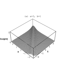
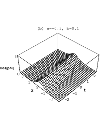
Figure 3: $\cos\varphi$ for (a) one-soliton and (b) its chirally transformed soliton.

The other type of discrete symmetry of the action in Eq. (2.36) is the dual symmetry: [30]

$$\beta\leftrightarrow-\beta\ ,\ g\leftrightarrow i\sigma g$$ (5.32)

where $\sigma$ is a constant matrix with a property, $\sigma T+T\sigma=0$. For example, $\sigma=\sigma_{1}$ of Pauli matrices in the $SU(2)/U(1)$ case. This rather unconventional symmetry, also the name, stems from the ubiquitous nature of the action in Eq. (2.36), i.e. it also arises as a large level limit of parafermions in statistical physics and the above transform is an interchange between the spin and the dual spin variables [19]. In general, the change of the sign of $\beta$ makes the potential upside down so that the degenerate vacua becomes maxima of the potential and vice versa. Therefore, the dual transformed solutions are no longer stable solutions. This allows us to find a localized solution which approches to the maximum of the potential asymptotically (so called a “dark” soliton). In practice, the dark soliton for positive $\beta$ can be obtained by replacing $\beta\rightarrow-\beta\ ,\ \bar{z}\rightarrow-\bar{z}$ in the “bright” soliton of the negative $\beta$ case. For example, we obtain the dark 1-soliton for the $SU(2)/U(1)$ case as follows:

$$\cos{\varphi}e^{2i\eta} = -{b\over\sqrt{(a-\xi)^{2}+b^{2}}}\mbox{tanh}(2bz+2bC\bar{z})-i{a-\xi\over\sqrt{(a-\xi)^{2}+b^{2}}}$$

$$\theta = -2(a-\xi)(z-C\bar{z})-2\xi z.$$ (5.33)

Fig. 4 shows profiles of a dark soliton. Note that field intensity $|E|$ is the same as that of the bright soliton in Fig. 2. However, the population inversion $D$ for the dark soliton becomes inverted compared to that of the bright soliton.

Figure 4: Plots of $\phi$, $\theta$ , $D$ and $|E|$ for dark one-soliton with $b=2,~{}\xi$=0 . The plot is w.r.t. $x=2bz+2bC_{1}\bar{z}$. Real ($a=0$) and dashed ($a=3$) lines represent the topological and the nontopological solitons.

6 Discussion

In this paper, we have introduced a potential concept to optical systems described by the Maxwell-Bloch equation. In terms of the matrix potential, a field theory action for the Maxwell equation was established where the Bloch eqaution became a mere identity. Various identifications of multi-level systems have been made in associated with specific symmetric spaces $G/H$ and the resulting group theoretic properties have been used in constructing conserved integrals. The field theory action uncovered several new features of the Maxwell-Bloch system; gauge symmetry, topological and nontopological charges, self-detuning, modified area theorem etc.. In doing so, the introduction of a matrix potential variable $g$ was an essential step. One immediate question is about the generality of such a potential variable in the description of nonlinear optics problems. Throughout the paper, we have confined ourselves only to the integrable Maxwell-Bloch equations which admit the inverse scattering method. Also, we have concentrated only on the classical aspect of the field theory which gives a semi-classical description of light-matter interaction. In general, the Maxwell-Bloch equation is not integrable. Even the integrable cases require specific physical settings. For example, in the three-level system, integrability requires equal oscillator strengths. However, we emphasize that integrability is not a necessary condition for the matrix potential formalism. Even for nonintegrable cases, one could still solve the Bloch equation in terms of a matrix potential $g$, and express the Maxwell equation in terms of $g$ [23]. One example is the $2\rightarrow 2$ transition in the degenerate two-level system which is described by the double sine-Gordon equation when certain restrictions are made. A more general matrix potential treatment of nonintegrable cases will be considered elsewhere.

On the other hand, the group theoretic approach in terms of $g$ is not restricted to the Maxwell-Bloch systems only. The nonlinear Schrödinger equation, which is the governing equation for optical soliton communication systems, can be generalized according to each Hermitian symmetric spaces [33]. In fact, both the Maxwell-Bloch and the nonlinear Schrödinger equations share the same Hamiltonian structure and they can be combined together. This case and its physical applications will be considered in a separate paper. Finally, we point out that our field theory formulation provides a vantage point to the quantum Maxwell-Bloch system as well as the quantum optics itself. A direct quantization of the Maxwell-Bloch equation using the quantum inverse scattering has been made by Rupasov and a localized multiparticle state has been found and compared with a quantum soliton [34]. Our field theory formulation suggests an alternative, yet more systematic way of quantization through the use of quantum field theory. The appearance of specific coset structures and their Hermitian properties suggests that a systematic quantization based on group theory is possible. Once again, this is not restricted to integrable cases and extensions to other quantum optical systems can be made. This work is in progress and will be reported elsewhere.

ACKNOWLEDGEMENT This work was supported in part by Korea Science and Engineering Foundation (KOSEF) 971-0201-004-2, and by the program of Basic Science Research, Ministry of Education BSRI-97-2442, and by KOSEF through CTP/SNU. APPENDIX A: Inverse scattering method and the matrix potential In the following, we show that the matrix potential is intimately related to the dressing (inverse scattering) method and explain how to obtain exact solutions. The dressing method is a systematic way to obtain nontrivial solutions from a trivial one. In our case, we take a trivial solution by

$$g=1\mbox{ and }\Psi=\Psi^{0}\equiv\exp[-(A-\xi T+\tilde{\lambda}T)z-\left<{\bar{T}\over\tilde{\lambda}-\xi^{{}^{\prime}}}\right>\bar{z}].$$ (A.1)

Let $\Gamma$ be a closed contour or a contour extending to infinity on the complex plane of the parameter $\tilde{\lambda}$ and $G(\tilde{\lambda})$ be a matrix function on $\Gamma$. Consider the Riemann problem of $\Psi^{0}G(\tilde{\lambda})(\Psi^{0})^{-1}$ on $\Gamma$ which consists of the factorization

$$\Psi^{0}G(\tilde{\lambda})(\Psi^{0})^{-1}=(\Phi_{-})^{-1}\Phi_{+}$$ (A.2)

where the matrix function $\Phi_{+}(z,\bar{z},\tilde{\lambda})$ is analytic with $n$ simple poles $\mu_{1},...,\mu_{n}$ inside $\Gamma$ and $\Phi_{-}(z,\bar{z},\tilde{\lambda})$ analytic with $n$ simple zeros $\lambda_{1},...,\lambda_{n}$ outside $\Gamma$. We assume that none of these poles and zeros lie on the contour $\Gamma$ and the factorization is analytically continued to the region where $\lambda\neq\mu_{i},\lambda_{i}\ ;\ i=1,...,n$. We normalize $\Phi_{+},\Phi_{-}$ by $\Phi_{+}|_{{\tilde{\lambda}}=\infty}=\Phi_{-}|_{{\tilde{\lambda}}=\infty}=1$. Differentiating Eq. (A.2) with respect to $z$ and $\bar{z}$, one can easily show that

$$\partial\Phi_{+}\Phi_{+}^{-1}-\Phi_{+}(A-\xi T+\tilde{\lambda}T)\Phi_{+}^{-1} = \partial\Phi_{-}\Phi_{-}^{-1}-\Phi_{-}(A-\xi T+\tilde{\lambda}T)\Phi_{-}^{-1}$$

$$\bar{\partial}\Phi_{+}\Phi_{+}^{-1}-\left<{\Phi_{+}\bar{T}\Phi_{+}^{-1}\over\tilde{\lambda}-\xi^{{}^{\prime}}}\right> = \bar{\partial}\Phi_{-}\Phi_{-}^{-1}-\left<{\Phi_{-}\bar{T}\Phi_{-}^{-1}\over\tilde{\lambda}-\xi^{{}^{\prime}}}\right>.$$ (A.3)

Since $\Phi_{+}(\Phi_{-})$ is analytic inside(outside) $\Gamma$, we find that the matrix functions $\bar{U}$ and $\bar{V}$, defined by

$$\bar{U} \equiv -\partial\Phi\Phi^{-1}+\Phi(A-\xi T+\tilde{\lambda}T)\Phi^{-1}-\tilde{\lambda}T$$

$$\bar{V} \equiv -(\tilde{\lambda}-\xi)\bar{\partial}\Phi\Phi^{-1}+\Phi\bar{T}\Phi^{-1}$$ (A.4)

where $\Phi=\Phi_{+}$ or $\Phi_{-}$ depending on the region, become independent of $\tilde{\lambda}$. Then, $\Psi\equiv\Phi\Psi^{0}$ satisfies the linear equation;

$$(\partial+\bar{U}+\tilde{\lambda}T)\Psi=0\ ,\ (\bar{\partial}+\left<{\bar{V}\over\tilde{\lambda}-\xi^{{}^{\prime}}}\right>)\Psi=0\ .$$ (A.5)

Since $\bar{U},\bar{V}$ are independent of $\tilde{\lambda}$, we may fix $\tilde{\lambda}$ by taking $\tilde{\lambda}=\xi$. Define $g$ by $g\equiv H\Phi^{-1}|_{\tilde{\lambda}=\xi}$ where $H$ is an arbitrary constant matrix which commutes with $T,\bar{T}$ and $A$. Then, $\bar{U}$ and $\bar{V}$ become

$$\bar{U} = g^{-1}\partial g+g^{-1}Ag-\xi T$$ (A.6)

$$\bar{V} = g^{-1}\bar{T}g.$$ (A.7)

If we further require the constraint condition (2.45) on $\Phi^{-1}|_{\tilde{\lambda}=\xi}$ such that

$$(-\partial\Phi\Phi^{-1}+\Phi A\Phi^{-1})_{\bf h}-A=0,$$ (A.8)

we obtain a nontrivial solution $g$ and $\Psi$ from a trivial one. The nontrivial solution in general describes n-solitons coupled with radiation mode. If $G(\tilde{\lambda})=1$ in Eq. (A.2), we obtain exact n-soliton solutions. This formal procedure may be carried out explicitly for each cases of SIT in Sec. 3 and a closed form of n-soliton solutions can be obtained. APPENDIX B: Conserved local integrals We first review some basic facts about Hermitian symmetric space [22] which are relevant for the construction of conserved integrals. A symmetric space $G/H$ is a coset space with the Lie algebra commutation relations among generators of associated Lie algebras such that

$$[\bf{h}\ ,\ \bf{h}]\subset\bf{h}\ ,\ [\bf{h}\ ,\ \bf{m}]\subset\bf{m}\ ,\ [\bf{m}\ ,\ \bf{m}]\subset\bf{h}\ ,$$ (B. 1)

where $\bf{g}$ and $\bf{h}$ are Lie algebras of $G$ and $H$ and $\bf{m}$ is the vector space complement of $\bf{h}$ in $\bf{g}$, i.e.

$$\bf{g}=\bf{h}\oplus\bf{m}.$$ (B. 2)

Hermitian symmetric space is a symmetric space equipped with a complex structure. In general, such a complex structure is given by the adjoint action of $T_{0}$ on ${\bf m}$ up to a scaling, where $T_{0}$ is an element belonging to the Cartan subalgebra of ${\bf g}$ whose stability subgroup is $H$. In our case, $T_{0}$ is precisely the $T$-matrix given in Sec. 3. Namely, with a suitable normalization of $T$, we have

$$T\in{\bf h}\ \ ,\ \ [T\ ,\ {\bf h}]=0\ \ \mbox{ and }\ \ [T\ ,\ [T\ ,\ a]]=-a\ \mbox{ for any }a\in{\bf m}.$$ (B. 3)

We decompose an algebra element $\psi\in{\bf g}$ according to Eq. (B. 2),

$$\psi=\psi_{h}+\psi_{m}.$$ (B. 4)

Such a decomposition could be extended to a representation $\Psi$ of $G=SU(n)$ if we substitute the commutator by a direct matrix multiplication and add an identity element $h_{0}=I$ to the subalgebra ${\bf h}$, i.e.

$$\Psi=\Psi_{h}+\Psi_{m},~{}~{}~{}\Psi_{h}\Psi_{h}\subset\Psi_{h},~{}~{}\Psi_{h}\Psi_{m}\subset\Psi_{m},~{}~{}\Psi_{m}\Psi_{m}\subset\Psi_{h}.$$ (B. 5)

In other words, any unitary $n\times n$ matrix can be expressed as a linear combination of $SU(n)$ generators and the identity element $h_{0}$ such that

$$\Psi=\Psi_{h}+\Psi_{m}=\sum_{a=0}^{\mbox{dim }\bf h}\Psi_{h}^{a}h_{a}+\sum_{b=1}^{\mbox{dim }\bf m}\Psi_{m}^{b}m_{b}.$$ (B. 6)

In order to solve the linear equation (2.46) recursively, we expand $\Psi$ in terms of a power series in ${\lambda}$,

$$\Psi\exp(-{{\lambda}}Tz)=\sum_{i=0}^{\infty}{1\over{{\lambda}}^{i}}\Phi_{i},$$ (B. 7)

where

$$\Phi_{i}=\sum_{a=0}^{\mbox{dim }\bf h}\Phi_{hi}^{a}h_{a}+\sum_{b=1}^{\mbox{dim }\bf m}\Phi_{mi}^{b}m_{b}\equiv{\cal X}_{i}+{\cal Y}_{i}.$$ (B. 8)

With the notation in Eq. (5.16), the linear equation is given by

$$(\partial+{\cal E})\Phi_{i}-[T\ ,\ \Phi_{i+1}]=0$$ (B. 9)

and

$$\bar{\partial}\Phi_{i}+\sum_{l=0}^{i-1}(D_{i-l-1}+P_{i-l-1})\Phi_{l}=0.$$ (B. 10)

Then, the $\bf{m}$-component of Eq. (B. 9) is

$$\partial{\cal Y}_{i-1}+{\cal E}{\cal X}_{i-1}-[T\ ,\ {\cal Y}_{i}]=0,$$ (B. 11)

which can be solved for ${\cal Y}_{i}$ by applying the adjoint action of $T$,

$${\cal Y}_{i}=-[T\ ,\ \partial{\cal Y}_{i-1}]-[T\ ,\ {\cal E}]{\cal X}_{i-1}.$$ (B. 12)

${\cal X}_{i}$ can be solved similarly from the $\bf{h}$-component of Eqs. (B. 9) and (B. 10) such that

$${\cal X}_{i}=-\int{\cal E}{\cal Y}_{i}dz-\sum_{l=0}^{i-1}\int(D_{i-l-1}{\cal X}_{l}+P_{i-l-1}{\cal Y}_{l})d\bar{z}.$$ (B. 13)

Finally, the conserved current follows from the consistency condition $\partial\bar{\partial}{\cal X}_{i}=\bar{\partial}\partial{\cal X}_{i}$.

With the repetitive use of the properties of the Hermitian symmetric space, it can be easily checked that these conservation laws are indeed consistent with the equations of motion (2.47) and (2.48), which in the present convention take a particularly simple form:

$$\bar{\partial}{\cal E}+[T~{},~{}P_{0}] = 0$$

$$\partial D_{i}+[{\cal E}~{},~{}P_{i}] = 0$$

$$\partial P_{i}+[{\cal E}~{},~{}D_{i}]-[T\ ,\ P_{i+1}] = 0.$$ (B. 14)

In general, the conserved current contains nonlocal terms. These nonlocal terms may be dropped out by taking the $T$-component of the currents. For instance, the $T$-component of the “spin-2” current conservation is

$$\bar{\partial}{\rm Tr}(T{\cal E}\partial{\cal E})=\partial{\rm Tr}(TP_{0}[T\ ,\ {\cal E}]-TD_{1})$$ (B. 15)

which obviously does not contain nonlocal terms.

References

- [1] O. Kocharovskaya and Ya.I. Khanin, JETP Lett. 48. 581 (1988); S.E. Harris, Phys. Rev. Lett. 62, 1033 (1989); M.O. Scully, S.-Y. Zhu, and A. Gavrielides, Phys. Rev. Lett. 62, 2813 (1989).
- [2] A.S. Zibriv et al., Phys. Rev. Lett. 75, 1499 (1995); G.G. Padmadandu et al., Phys. Rev. Lett. 76, 2053 (1996).
- [3] K.J. Boller, A. Imamoglu, and S.E. Harris, Phys. Rev. Lett. 66 2593 (1991).
- [4] S. L. McCall and E. L. Hahn, Phys. Rev. Lett. 18, 908 (1967); Phys. Rev. 183, 457 (1969).
- [5] A. Leclair, F. Lesage, S. Lukyanov and H. Saleur,“The Maxwell-Bloch theory in quantum optics and the Kondo model” hep-th/971022; A. Leclair, “Eigenstates of the atom-field interaction and the binding of light in photonic crystals” hep-th/9706150.
- [6] Q-H. Park and H.J. Shin, J. Korean. Phys. Soc. 30, 336 (1997).
- [7] A. I. Maimistov, A. M. Basharov, S. O. Elyutin and Yu. M. Sklyarov, Phys. Rep. 191, No. 1 , 1-108 (1990).
- [8] G. L. Lamb, Jr., Phys. Rev. Lett. 31, 196 (1973).
- [9] M. J. Ablowitz, D. J. Kaup and A. C. Newell, J. Math. Phys. 15, 1852 (1974).
- [10] A.I. Maimistov, Opt. Spektrosk. 57, 564 (1984).
- [11] A.M. Bashrov and A.M.Maimstov, Sov. Phys. JETP 60, 913 (1984).
- [12] A.M. Bashrov and A.M.Maimstov, Sov. Phys. JETP 67, 2426 (1988).
- [13] F. Lund and T. Regge, Phys. Rev. D14, 1524 (1976).
- [14] K. Pohlmeyer, Commun. Math. Phys. 46, 207 (1976).
- [15] F. Bloch, Phys. Rev. 70, 460 (1946).
- [16] E. Witten, Commun. Math. Phys. 92, 455 (1984).
- [17] D.Karabali, Q-H.Park, H.J.Schnitzer and Z.Yang, Phys. Lett. B216, 307 (1989); K.Gawedski and A.Kupiainen,, Nucl. Phys. B320, 625 (1989).
- [18] I. Bakas, Int. J. Mod. Phys. A9, 3443 (1994).
- [19] Q-H. Park, Phys. Lett. B328, 329 (1994).
- [20] Q-H. Park and H. J. Shin, Phys. Lett. B347, 73 (1995); Nucl. Phys. B458, 327 (1996); T. J. Hollowood, J. L. Miramontes and Q-H. Park, Nucl. Phys. B445, 451 (1995).
- [21] I. Bakas, Q-Han Park and H. J. Shin, Phys. Lett. B372, 45 (1996).
- [22] S. Helgason, Differential geometry, Lie groups and symmetric spaces. 2nd ed. New York; Academic Press 1978.
- [23] Q-H. Park and H.J. Shin, “Matched pulse propagation in a three-level system”
- [24] S.E. Harris, Phys. Rev. Lett. 72, 52 (1994).
- [25] J.H. Eberly, M.L. Pons, and H.R. Haq, Phys. Rev. Lett. 72, 56 (1994).
- [26] S.E. Harris and Z. Luo, Phys. Rev. A 52, R928 (1995).
- [27] G. Vemuri, K.V. Vasavada, G.S. Agarwal, and Q. Zhang, Phys. Rev. A 54, 3394 (1996).
- [28] G. Vemuri, K.V. Vasavada, Optics Comm. 129, 379 (1996).
- [29] A.M. Basharov, Sov. Phys. JETP 70, 94 (1990).
- [30] Q-H. Park and H. J. Shin, Phys. Lett. B359, 125 (1995).
- [31] J.C. Diels, Phys. Lett. A 31, 111 (1970).
- [32] G.L. Lamb, Jr., Rev. Mod. Phys. 43, 99 (1971).
- [33] A.P. Fordy and P.P. Kulish, Commum. Math. Phys. 89, 427 (1983);P. Oh and Q-H. Park, Phys. Lett. 383B, 333 (1996).
- [34] V.I. Rupasov, Pis’ma Zh. Eksp. Teor. Fiz. 36, 115 (1982); Sov. Phys. JETP 56, 989 (1982).