Optimal signal ensembles

⁽¹⁾Department of Physics, Kenyon College, Gambier, OH 43022 USA
⁽²⁾Department of Mathematical Sciences, Denison University, Granville, OH 43023 USA

Abstract

Classical messages can be sent via a noisy quantum channel in various ways, corresponding to various choices of ensembles of signal states of the channel. Previous work by Holevo and by Schumacher and Westmoreland relates the capacity of the channel to the properties of the signal ensemble. Here we describe some properties characterizing the ensemble that maximizes the capcity, using the relative entropy “distance” between density operators to give the results a geometric flavor.

1 Communication via quantum channels

Suppose Alice wishes to send a (classical) message to Bob, using a quantum system as the communication channel. Alice prepares the system in the “signal state” $\rho_{k}$ with probability $p_{k}$, so that the ensemble of states is described by an average density operator $\rho={\displaystyle\sum_{k}}p_{k}\,\rho_{k}$. Bob makes a measurement of a “decoding observable” on the system and uses the result to infer which signal state was prepared. The choice of system preparation (represented by the index $k$) and Bob’s measurement outcome are the input and output of a classical communication channel.

Holevo [1] proved (as Gordon [2] and Levitin [3] had previously conjectured) that the mutual information between the input and output of this channel, regardless of Bob’s choice of decoding observable, can never be greater than $\chi$, where

$$\chi=S(\rho)-\sum_{k}p_{k}S(\rho_{k})$$ (1)

where $S(\rho)=-\mbox{Tr}\,\rho\log\rho$ is the von Neumann entropy of the density operator $\rho$.

More recently, it has been shown by Holevo [4] and by Schumacher and Westmoreland [5] that the Holevo bound is asymptotically achievable. That is, if Alice uses many copies of the same channel, preparing long code words of signal states, and if Bob chooses an entangled decoding observable, Alice can convey to Bob up to $\chi$ bits of information per use of the channel, with arbitrarily low probability of error. (This fact was first shown for pure state signals in [6].)

Suppose the channel is a noisy one described by a superoperator ${\cal E}$. Then if Alice prepares the input signal state $\rho_{k}$, Bob will receive the output signal state ${\cal E}(\rho_{k})$. It is the ensemble of output signal states that determines the capacity of the channel. Effectively, the superoperator ${\cal E}$ restricts the set of signals that Alice can present to Bob for decoding. If $\cal B$ is the set of all density operators, then Alice’s efforts can only produce output states in the set $\mbox{$\cal A$}={\cal E}({\cal B})$.

In this paper we will consider the problem of maximizing $\chi$ for ensembles of states drawn from a given set $\cal A$ of available states. This includes the problem of maximizing $\chi$ for the outputs of a noisy channel, if $\cal A$ is chosen to be the set of possible channel outputs. In this case, $\cal A$ will be a convex set; but we will not need the convexity of $\cal A$ for many of our results.

2 Relative entropy

If $\rho$ and $\sigma$ are density operators, then the relative entropy of $\rho$ with respect to $\sigma$ is defined to be

$${\cal D}\left(\rho||\sigma\right)=\mbox{Tr}\,\rho\log\rho-\mbox{Tr}\,\rho\log\sigma.$$ (2)

Here are three important points about the relative entropy:

• ${\cal D}\left(\rho||\sigma\right)\geq 0$, with equality if and only if $\rho=\sigma$.

• Strictly speaking, ${\cal D}\left(\rho||\sigma\right)$ is defined only if $\mbox{supp}\,\rho\subseteq\mbox{supp}\,\sigma$ (where “$\mbox{supp}\,\rho$” is the support of the operator $\rho$). If this is not the case, then we take ${\cal D}\left(\rho||\sigma\right)=\infty$. For example, if $\rho$ and $\sigma$ are distinct pure states, the relative entropy is always infinite.

• The relative entropy is jointly convex in its arguments:

  $${\cal D}\left(p_{1}\rho_{1}+p_{2}\rho_{2}||p_{1}\sigma_{1}+p_{2}\sigma_{2}\right)\leq p_{1}{\cal D}\left(\rho_{1}||\sigma_{1}\right)+p_{2}{\cal D}\left(\rho_{2}||\sigma_{2}\right)$$ (3)

  for $p_{1},p_{2}\geq 0$ with $p_{1}+p_{2}=1$. From this fact it also follows that the relative entropy is convex in each of its arguments.

The relative entropy plays a role in the asymptotic distinguishability of quantum states by measurement [7], and has been used to develop measures of quantum entanglement [8]

It is often convenient to think of the relative entropy ${\cal D}\left(\rho||\sigma\right)$ as a “directed distance” from $\sigma$ to $\rho$, even though it lacks some of the properties of a true metric. This view of the relative entropy will let us give a geometric interpretation to our results.

Suppose as before we have an ensemble of signal states in the available set $\cal A$, in which $\rho_{k}$ appears with probability $p_{k}$. It is easy to verify that the Holevo bound $\chi$ can be given in terms of the relative entropy:

$$\chi=\sum_{k}p_{k}{\cal D}\left(\rho_{k}||\rho\right).$$ (4)

That is, $\chi$ is just the average of the relative entropy of the members of the signal ensemble with respect to the average signal state.

3 The optimal signal ensemble

To maximize the information capacity of the channel, Alice will want to choose a signal ensemble that maximizes $\chi$. We will denote the maximum of $\chi$ for a given set $\cal A$ of available states by $\chi^{*}$. Any ensemble of signal states that achieves this value of the Holevo bound will be called an optimal signal ensemble.

If the set of available states $\cal A$ is a closed convex set, then we can always take an optimal ensemble to be composed of extreme points of $\cal A$—that is, states which cannot be written as convex sums of other states in $\cal A$. To see this, suppose we have an ensemble of $\cal A$-states with average state $\rho$, and further suppose that $\rho_{k}$ is a member of the ensemble that is not an extreme point. This means that there are states $\rho_{k0}$ and $\rho_{k1}$ in $\cal A$ such that

$$\rho_{k}=q_{0}\rho_{k0}+q_{1}\rho_{k1}$$ (5)

for probabilities $q_{0}$ and $q_{1}$ that sum to unity. By the convexity of the relative entropy,

$${\cal D}\left(\rho_{k}||\rho\right)\leq q_{0}{\cal D}\left(\rho_{k0}||\rho\right)+q_{1}{\cal D}\left(\rho_{k1}||\rho\right).$$ (6)

Since $\chi$ is the average of the relative entropies, we will never make $\chi$ smaller by replacing $\rho_{k}$ (with probability $p_{k}$) by $\rho_{k0}$ and $\rho_{k1}$ (with probabilities $p_{k}q_{0}$ and $p_{k}q_{1}$, respectively) in the ensemble. Thus, at least one optimal ensemble will be composed of extreme points of $\cal A$.

For noisy channels, this means that pure state inputs to the channel are optimal – that is, it never increases $\chi$ to use mixed states as inputs. This fact was shown in [5].

A second and very surprising fact was discovered by Fuchs [9]. The quantity $\chi$ is a measure of the distinguishability of an ensemble of signal states. If we wish to maximize the distinguishability of the output signals of a noisy channel, we might imagine that we should always maximize the distinguishability of the input signals—i.e., choose an orthogonal set of input states. But this intuition turns out to be false.

Some insight can be gained by examining a specific counter-example. Our quantum system is a spin, and $\left|\uparrow\right\rangle$ and $\left|\downarrow\right\rangle$ represent eigenstates of $S_{z}$. The spin is subject to “amplitude damping”, so that an initial density operator $\rho$ evolves into a density operator

$$\rho^{\prime}={\cal E}(\rho)=A_{1}\rho A_{1}^{\dagger}+A_{2}\rho A_{2}^{\dagger}$$ (7)

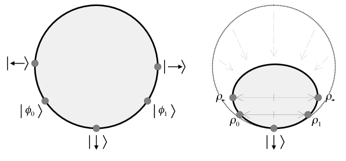
Figure 1: Bloch sphere diagram for amplitude damping. The highest value of $\chi$ for a set of orthogonal input signals is attained by an equally weighted mixture of $\left|\rightarrow\right\rangle$ and $\left|\leftarrow\right\rangle$, but the non-orthogonal input signals $\left|\phi_{0}\right\rangle$ and $\left|\phi_{1}\right\rangle$ yield a larger value of $\chi$.

where $A_{1}=\sqrt{1-\lambda}\left|\uparrow\right\rangle\!\left\langle\uparrow\right|+\left|\downarrow\right\rangle\!\left\langle\downarrow\right|$ and $A_{2}=\sqrt{\lambda}\left|\downarrow\right\rangle\!\left\langle\uparrow\right|$, and $0\leq\lambda\leq 1$. The result of this operation is, for instance, to leave the state $\left|\downarrow\right\rangle$ unchanged but to cause $\left|\uparrow\right\rangle$ to decay to $\left|\downarrow\right\rangle$ with probability $\lambda$. We choose $\lambda=1/2$. A diagram of this process in the Bloch sphere is found in Figure 1.

If we consider only orthogonal input signal ensembles, the maximum $\chi$ is obtained for an equally weighted ensemble of $\left|\rightarrow\right\rangle$ and $\left|\leftarrow\right\rangle$, for which $\chi=0.4567$ bits. But a non-orthogonal ensemble of the states $\left|\phi_{0}\right\rangle$ and $\left|\phi_{1}\right\rangle$ can achieve $0.4717$ bits, where the angle in Hilbert space between the two inputs is about 80^∘.

Why is this? Recall that $\chi$ is the average relative entropy “distance” from the average signal state to the individual signal states. This distance function grows larger near the boundary of the Bloch sphere–so that, for example, the relative entropy distance between distinct pure states is infinite. Thus, despite the appearance in Figure 1, the relative entropy distances for the ensemble of $\rho_{0}$ and $\rho_{1}$ are greater than those for the ensemble of $\rho_{\rightarrow}$ and $\rho_{\leftarrow}$.

4 Changing the ensemble

In this section we will prove some useful results that will enable us to further characterize the optimal ensembles for a given set $\cal A$ of available states.

Suppose as before that the signal state $\rho_{k}\in\mbox{$\cal A$}$ appears in our ensemble with probability $p_{k}$, yielding an average state $\rho$. Let $\sigma$ be some other density operator, which we will call the “alternate” state. Then we can calculate the average relative entropy distance of the signal states from $\sigma$:

$$\sum_{k}p_{k}{\cal D}\left(\rho_{k}||\sigma\right) = \sum_{k}p_{k}\left(\mbox{Tr}\,\rho_{k}\log\rho_{k}-\mbox{Tr}\,\rho_{k}\log\sigma\right)$$

$$= \sum_{k}p_{k}\left(\mbox{Tr}\,\rho_{k}\log\rho_{k}-\mbox{Tr}\,\rho_{k}\log\rho\right)$$

$$+\left(\mbox{Tr}\,\rho\log\rho-\mbox{Tr}\,\rho\log\sigma\right)$$

$$= \sum_{k}p_{k}{\cal D}\left(\rho_{k}||\rho\right)+{\cal D}\left(\rho||\sigma\right)$$

$$\sum_{k}p_{k}{\cal D}\left(\rho_{k}||\sigma\right) = \chi+{\cal D}\left(\rho||\sigma\right).$$ (8)

This useful identity, first given by Donald[10], has a number of implications. For example,

• For any ensemble and any $\sigma$,

  $$\sum_{k}p_{k}{\cal D}\left(\rho_{k}||\sigma\right)\geq\chi$$ (9)

  with equality if and only if $\sigma=\rho$.

• From the previous point it follows that

  $$\chi=\min_{\sigma}\left(\sum_{k}p_{k}{\cal D}\left(\rho_{k}||\sigma\right)\right)$$ (10)

  where the minimum is taken over all density operators $\sigma$.

Now we will use our identity to consider how the value of $\chi$ would change if we were to modify our ensemble. In particular, we can introduce a new state $\rho_{0}$ with probability $\eta$, shrinking the other probabilities to maintain normalization. We may conveniently refer to our ensembles as the “original” and “modified” ensembles, as summarized in the following table:

ensemble	original	modified
signal states	$\rho_{k}$	$\rho_{k},\rho_{0}$
probabilities	$p_{k}$	$(1-\eta)p_{k},\eta$
average state	$\rho$	$\rho^{\prime}$
Holevo bound	$\chi$	$\chi^{\prime}$

where

$$\rho^{\prime} = (1-\eta)\rho+\eta\rho_{0}$$ (11)

$$\chi = \sum_{k}p_{k}{\cal D}\left(\rho_{k}||\rho\right)$$ (12)

$$\chi^{\prime} = (1-\eta)\sum_{k}p_{k}{\cal D}\left(\rho_{k}||\rho^{\prime}\right)\,\,+\,\,\eta{\cal D}\left(\rho_{0}||\rho^{\prime}\right).$$ (13)

We wish to find how the Holevo bound changes – that is, we wish to make an estimate of $\Delta\chi=\chi^{\prime}-\chi$.

Begin with the expression for $\chi^{\prime}$ and apply Equation 8, choosing the original ensemble and letting the modified average state $\rho^{\prime}$ play the role of the alternate state. This yields

$$\chi^{\prime} = (1-\eta)\left(\chi+{\cal D}\left(\rho||\rho^{\prime}\right)\right)+\eta{\cal D}\left(\rho_{0}||\rho^{\prime}\right)$$

$$= \chi+\eta\left({\cal D}\left(\rho_{0}||\rho^{\prime}\right)-\chi\right)+(1-\eta){\cal D}\left(\rho||\rho^{\prime}\right)$$

$$\Delta\chi = \eta\left({\cal D}\left(\rho_{0}||\rho^{\prime}\right)-\chi\right)+(1-\eta){\cal D}\left(\rho||\rho^{\prime}\right).$$

Therefore,

$$\Delta\chi\geq\eta\left({\cal D}\left(\rho_{0}||\rho^{\prime}\right)-\chi\right).$$ (14)

This gives us a lower bound for $\Delta\chi$.

To obtain an upper bound, we apply Equation 8 to the modified ensemble, with the original average state $\rho$ playing the role of the alternate state.

$$\chi^{\prime}+{\cal D}\left(\rho^{\prime}||\rho\right) = (1-\eta)\left(\sum_{k}p_{k}{\cal D}\left(\rho_{k}||\rho\right)\right)+\eta{\cal D}\left(\rho_{0}||\rho\right)$$

$$= (1-\eta)\chi+\eta{\cal D}\left(\rho_{0}||\rho\right)$$

$$\chi^{\prime}-\chi = \eta\left({\cal D}\left(\rho_{0}||\rho\right)-\chi\right)-{\cal D}\left(\rho^{\prime}||\rho\right)$$

And so we obtain

$$\Delta\chi\leq\eta\left({\cal D}\left(\rho_{0}||\rho\right)-\chi\right).$$ (15)

In deriving this inequality, we obviously assume that $\mbox{supp}\,\rho_{0}\subseteq\mbox{supp}\,\rho$. But if this is not the case, then the inequality still holds in the sense that the right-hand side is infinite.

It is easy to generalize these results to a situation in which we modify the ensemble by adding many states. Suppose the states $\rho_{0a}$ are added with probabilities $\eta q_{a}$ (where the $q_{a}$’s form a probability distribution). Then the above results would become

$$\eta\left(\sum_{k}q_{a}{\cal D}\left(\rho_{0a}||\rho^{\prime}\right)-\chi\right)\leq\Delta\chi\leq\eta\left(\sum_{k}q_{a}{\cal D}\left(\rho_{0a}||\rho\right)-\chi\right).$$ (16)

All of our subsequent results still hold in this more general situation, but to simplify the discussion we will phrase our arguments in terms of “single state” modifications of a given ensemble.

Finally, consider states $\rho_{0}$ and $\rho$, and let $\rho^{\prime}=(1-\eta)\rho+\eta\rho_{0}$. Then ${\cal D}\left(\rho_{0}||\rho^{\prime}\right)$ exists and is finite for $0<\eta\leq 1$, and

• If $\mbox{supp}\,\rho_{0}\subseteq\mbox{supp}\,\rho$, then ${\cal D}\left(\rho_{0}||\rho^{\prime}\right)\rightarrow{\cal D}\left(\rho_{0}||\rho\right)$ as $\eta\rightarrow 0$.

• Otherwise, ${\cal D}\left(\rho_{0}||\rho^{\prime}\right)\rightarrow\infty$ as $\eta\rightarrow 0$.

We see that Equations 14 and 15 are fairly “tight” lower and upper bounds for $\Delta\chi$, because (informally speaking) the two expressions approach one another as $\eta$ approaches zero.

5 Properties of optimal ensembles

For a given set ${\cal A}$ of available states (e.g., the outputs of a noisy channel), let $\rho_{k}$ and $p_{k}$ be the members and probabilities of the ensemble of ${\cal A}$-states for which $\chi$ takes on its maximum value. Call this the “$\chi$-optimal ensemble”, and let $\rho^{\ast}$ be the average state of this ensemble. Denote $\max\chi$ by $\chi^{\ast}$. The $\chi$-optimal ensemble has a number of important properties.

Existence.

If the letter states are outputs of a noisy channel in a finite-dimensional Hilbert space, then a $\chi$-maximizing ensemble exists.

Proof: The key result can found in [11]: Let $\cal A$ be a convex, compact subset $\cal A$ of density operators on a Hilbert space of finite dimension $d$, and let $\rho$ be in $\cal A$. If the set of extremal elements of $A$ is compact then for any $\rho\in A$ there exists an ensemble of states $\{\rho_{k}\}\subset A$ with $\rho=\sum p_{k}\rho_{k}$ that maximizes $\chi$ over the set of all ensembles whose average state is $\rho$. In other words, there exist optimal signal ensembles for a given average state $\rho$. By Caratheodory’s Theorem, since the Hilbert space has $d$ dimensions, then there are optimal ensembles (in this sense) with no more than $d^{2}$ states.

We see that the conditions for the result from [11] are met. The set of states $\cal A$ that are possible outputs of the channel is a convex, compact set with a compact set of extremal points. For any average state $\rho$ in $\cal A$, we can find a $\rho$-fixed optimal ensemble with $d^{2}$ or fewer elements. Thus, in order to maximize $\chi$ over all possible ensembles, we only need to consider the set of ensembles with no more than $d^{2}$ elements drawn from $\cal A$. As this is a finite cartesian product of a compact set, it is compact. As $\chi$ is a continuous function, it must achieve its maximum in this set of ensembles. Thus, the existence of an optimal ensemble of states in $\cal A$ is assured.

Maximal distance property.

For any state $\rho_{0}$ in ${\cal A}$,

$${\cal D}\left(\rho_{0}||\rho^{\ast}\right)\leq\chi^{\ast}.$$ (17)

Proof. We assume the existence of a state $\rho_{0}$ with ${\cal D}\left(\rho_{0}||\rho^{\ast}\right)>\chi^{\ast}$. (We allow for the possibility that ${\cal D}\left(\rho_{0}||\rho^{\ast}\right)$ is infinite.) Since ${\cal D}\left(\rho_{0}||\rho^{\prime}\right)\rightarrow{\cal D}\left(\rho_{0}||\rho^{\ast}\right)$ as $\eta\rightarrow 0$, we can find a value of $\eta$ so that ${\cal D}\left(\rho_{0}||\rho^{\prime}\right)>\chi^{\ast}$. Then by Equation 14,

$$\Delta\chi\geq\eta\left({\cal D}\left(\rho_{0}||\rho^{\prime}\right)-\chi^{\ast}\right)>0.$$

That is, we can increase $\chi$ by including $\rho_{0}$ in the signal ensemble, which is a contradiction.

Maximal support property.

For a $\chi$-optimal ensemble, $\mbox{supp}\,\rho^{\ast}=\mbox{supp}\,{\cal A}$. (By “$\mbox{supp}\,{\cal A}$” we mean the smallest subspace that contains $\mbox{supp}\,\rho_{k}$ for any $\rho_{k}\in{\cal A}$.) In other words, any $\chi$-optimal ensemble “covers” the support of the set of available states.

Proof. This is a corollary to the maximum distance property. If there were a state $\rho_{0}\in{\cal A}$ so that $\mbox{supp}\,\rho_{0}$ were not contained in $\mbox{supp}\,\rho^{\ast}$, then ${\cal D}\left(\rho_{0}||\rho^{\ast}\right)$ would be infinite.

Sufficiency of maximal distance property.

Suppose we have an ensemble with average state $\rho$ and a particular value of $\chi$, and suppose that

$${\cal D}\left(\rho_{0}||\rho\right)\leq\chi$$

for all $\rho_{0}\in{\cal A}$. Then this must be a $\chi$-optimal ensemble. That is, the only ensembles that have the maximal distance property are $\chi$-optimal ensembles.

Proof: If we add a state $\rho_{0}$ with probability $\eta$ to the ensemble, then from Equation 15

$$\Delta\chi\leq\eta\left({\cal D}\left(\rho_{0}||\rho\right)-\chi\right)\leq 0$$

so that we cannot increase $\chi$. (By Equation 16, the same would hold if we were to add several different states instead of only one.) Thus, $\chi=\chi^{\ast}$.

Equal distance property.

Suppose $\rho_{k}$ is a member of a $\chi$-optimal ensemble with probability $p_{k}\neq 0$. Then

$${\cal D}\left(\rho_{k}||\rho^{\ast}\right)=\chi^{\ast}.$$ (18)

In other words, all of the non-zero members of a $\chi$-optimal ensemble have the same relative entropy “distance” with respect to the average state $\rho^{\ast}$.

Proof: This is another corollary to the maximal distance property. If ${\cal D}\left(\rho_{k}||\rho^{\ast}\right)<\chi^{\ast}$ for any $\rho_{k}$ with $p_{k}\neq 0$, then the average relative entropy cannot equal $\chi^{\ast}$.

Min-max formula for $\chi^{\ast}$.

From the above properties, we can show the following formula:

$$\chi^{\ast}=\min_{\rho}\left(\max_{\rho_{0}}{\cal D}\left(\rho_{0}||\rho\right)\right),$$ (19)

where the maximum is taken over all $\rho_{0}\in{\cal A}$ and the minimum is taken over all average states $\rho$ of ensembles of ${\cal A}$-states.

Proof: We first show that, for any state $\sigma$, the quantity $\displaystyle\max_{\rho_{0}}{\cal D}\left(\rho_{0}||\sigma\right)$ is an upper bound for the value of $\chi$ for any possible ensemble. By Equation 9, we find that

$$\chi\leq\sum_{k}p_{k}{\cal D}\left(\rho_{k}||\sigma\right)\leq\max_{\rho_{0}}{\cal D}\left(\rho_{0}||\sigma\right).$$

This will also hold for an optimal signal ensemble, for which $\chi=\chi^{\ast}$. Thus,

$$\chi^{\ast}\leq\min_{\rho}\left(\max_{\rho_{0}}{\cal D}\left(\rho_{0}||\rho\right)\right).$$

Next we note that the maximal distance property implies that

$$\chi^{\ast}=\max_{\rho_{0}}{\cal D}\left(\rho_{0}||\rho^{\ast}\right),$$

from which we can see that

$$\chi^{\ast}\geq\min_{\rho}\left(\max_{\rho_{0}}{\cal D}\left(\rho_{0}||\rho\right)\right).$$

These two inequalities establish the formula in Equation 19.

These properties provide strong characterizations of an optimal signal ensemble for a quantum channel. Equation 19, for example, shows that $\chi^{\ast}$ can be calculated as a purely “geometric” property of the set $\cal A$, without direct reference to any ensemble. We believe that our results are likely to prove useful in further investigations of the efficient use of quantum resources to transmit classical messages.

6 Acknowledgements

We would like to thank A. Uhlmann for helpful and enlightening comments, particularly about the existence of an optimal ensemble. We also had useful conversations with T. Cover, C. A. Fuchs, A. S. Holevo, V. Vedral and W. K. Wootters. Most of these discussions took place in connection with the programme on “Complexity, Computation and the Physics of Information” at the Isaac Newton Institute in Cambridge (England) during the summer of 1999. This programme was sponsored in part by the European Science Foundation. One of us (BS) gratefully acknowledges the support of a Rosenbaum Fellowship at the Isaac Newton Institute to participate in this programme.

References

- [1] A. S. Kholevo, Probl. Peredachi Inf. 9, 3 (1973) [Probl. Inf. Transm. (USSR) 9, 110 (1973)].
- [2] J. P. Gordon, in Quantum Electronics and Coherent Light, Proceedings of the International School of Physics “Enrico Fermi,” Course XXXI, edited by P. A. Miles (Academic, New York, 1964), pp. 156-181.
- [3] L. B. Levitin, “On the quantum measure of the amount of information,” in Proceedings of the IV National Conference on Information Theory, Tashkent, 1969, pp. 111–115 (in Russian); “Information Theory for Quantum Systems,” in Information, Complexity, and Control in Quantum Physics, edited by A. Blaquière, S. Diner, and G. Lochak (Springer, Vienna, 1987).
- [4] A. S. Holevo, IEEE Trans. Inform. Theory 44, 269 (1998).
- [5] B. Schumacher and M. Westmoreland, Phys. Rev. A 51, 2738 (1997).
- [6] P. Hausladen, R. Josza, B. Schumacher, M. Westmoreland and W. K. Wootters, Phys. Rev. A 54, 1869 (1996).
- [7] F. Hiai and D. Petz, Comm. Math. Phys. 143, 99 (1991). V. Vedral, M. B. Plenio, K. Jacobs and P. L. Knight, Phys. Rev. A 56, 4452 (1997).
- [8] V. Vedral, M. B. Plenio, M. A. Rippin and P. L. Knight, Phys. Rev. Lett. 78, 2275 (1997).
- [9] C. A. Fuchs, Phys. Rev. Lett. 79, 1162 (1997).
- [10] M. J. Donald, Math. Proc. Cam. Phil. Soc. 101, 363 (1987).
- [11] A. Uhlmann, Open Sys. and Inf. Dynamics 5, 209 (1998).