Time of arrival
through interacting environments:
Tunneling processes

Abstract

We discuss the propagation of wave packets through interacting environments. Such environments generally modify the dispersion relation or shape of the wave function. To study such effects in detail, we define the distribution function $P_{X}(T)$, which describes the arrival time $T$ of a packet at a detector located at point $X$. We calculate $P_{X}(T)$ for wave packets traveling through a tunneling barrier and find that our results actually explain recent experiments. We compare our results with Nelson’s stochastic interpretation of quantum mechanics and resolve a paradox previously apparent in Nelson’s viewpoint about the tunneling time.

1 Introduction

We are interested in the behavior of quantum particles, that is, wave packets propagating through interacting environment. In general, there are two types of environment. One is the ordinary medium (plasma, dielectric, etc.) which consists of “matter” [1-4]. The other is the nontrivial structure of the vacuum due to field theoretical fluctuations [5] or effects of quantum gravity [6, 7]. In both cases, the presence of such environments will modify the dispersion relation of particles, $E=f(p)$, or modify the shape of the wave packet. Observation of the arrival time of particles through such environments is a way to see the effects of these modifications. Recently, these effects have been tested in two fields, astrophysics and quantum optics. The first is the observation of arrival times of photons from distant astrophysical sources such as $\gamma$-ray bursters. Several models of quantum gravity suggest that the velocity of light has an effective energy dependence due to the modified dispersion relation induced by the nontrivial structure of space-time at distances comparable to the Planck length. To confirm this effect, it is necessary to observe a certain difference of the arrival time of photons with different energies, and $\gamma$-ray bursters work for this purpose [6]. As a result, a lower bound on the energy scale of quantum gravity is obtained [8]. The second recent test is observation of tunneling of photons. Chiao and co-workers constructed an elaborate stadium for the race between photons propagating in the vacuum and through an optical barrier, and measured their arrival times [1, 2]. They found that the photon tunneling through the barrier arrived at the goal earlier than the other photon traveling in the vacuum. Although this result implies superluminal velocity of the tunneling photon, it does not mean causality violation, because in this case the group velocity itself does not transport any information at all. The apparent superluminality results from reshaping of wave packets while tunneling. Similar phenomena can be found in absorbing media [9]. Anyway, in both experiments, measurement of the arrival time of wave packets plays an essential role.

However, there is no clear definition of arrival time in quantum mechanics. This has its root in the well-known fact that time is not an operator but a parameter in quantum mechanics. Though many authors have attempted to define an operator of arrival time and construct its eigenstates, a satisfactory formulation has not yet been obtained [10-25]. In this article we define a distribution function $P_{X}(T)$, which describes the arrival time of packets at a detector located at point $X$. In terms of $P_{X}(T)$, we can compute a mean arrival time $\left\langle T\right\rangle_{X}$. Of course we assume an ideal detector and our definition of $P_{X}(T)$ might not exactly correspond to the physical measurement process. However, concrete calculation of $P_{X}(T)$ shows us clearly the dynamical properties of propagation of packets through interacting environments.

We investigate the arrival time distribution $P_{X}(T)$ numerically for nonrelativistic massive particles traveling through a potential barrier in one space dimension, that is, tunneling processes. This might be a simple model for the experiment of Chiao and co-workers. In this case the existence of a potential barrier $V(x)$ causes reflection and transmission of packets; therefore the behavior of $P_{X}(T)$ will be highly nontrivial, depending on various parameters. How to deal with time in tunneling processes is also known as the tunneling time problem. The problem arises from the paradox that a particle under a potential greater than the particle’s energy seems to move with a purely imaginary velocity. In recent developments of nanotechnology, the study of the tunneling time has great significance because it might enable us to estimate the response time of nanodevices [27]. Various approaches to the tunneling time have been proposed by many authors [27-36]; however, it seems difficult to define it uniquely . Therefore we need to define effective tunneling times for each system and each purpose. We have no intention of wrestling with the general theory of tunneling time now; therefore, we restrict ourselves to analyzing the time of appearance of the packet in the exit of the potential barrier and how it moves after that. These two notions determining the arrival time difference have usually been confused. In this article we will distinguish them clearly.

Finally we consider the real-time stochastic interpretation of quantum mechanics introduced by Nelson [37]. Since it utilizes the real-time trajectories of quantum particles as sample paths, we can construct an appropriate time distribution from ensemble of sample paths. This is why Nelson’s approach is expected to be effective for time problems in quantum mechanics. In particular, it is interesting to attack the tunneling time problem from this approach because we can trace the particle’s real-time motion even under the tunneling potential. Actually it has been found that the tunneling particle “hesitates” in front of the barrier [38]. This property seems paradoxical because it implies that the particle tunneling through the barrier should always be delayed compared with the free one due to this hesitation and it seems contradictory to the advancement of the peak of the wave packet as seen in the experiment of Chiao and co-workers. Is it a real paradox?

It is clear that Nelson’s approach can reproduce any physical quantities of the usual quantum mechanics by averaging them about the sample path ensemble. However, there is no reason that any “observables” classically defined in Nelson’s stochastic procedures should have corresponding quantities in the standard quantum mechanics. We will compute the arrival time distribution in Nelson’s approach and compare it with our $P_{X}(T)$. Then we clarify the real physical meaning of the “hesitation” and show that there is no paradox at all. Furthermore, we mention that Nelson’s interpretation can explain the characteristic behavior of $\left\langle T\right\rangle_{X}$ for tunneling particles very well.

2 Definition of the arrival time distribution

First we will briefly review previous attempts to define a time of arrival operator and their difficulties. In the 1960s, Aharonov and Bohm quantized the representation of the classical arrival time for the free particle at a point $X=0$ [10],

$$T=-m\frac{x}{p}~{}~{}\rightarrow~{}~{}\hat{T}=-\frac{m}{2}\left(\hat{x}\frac{1}{\hat{p}}+\frac{1}{\hat{p}}\hat{x}\right).$$ (1)

Here $x$ and $p$ are the initial position and momentum, respectively, where we work in the Heisenberg picture. Because $\hat{T}$ satisfies $\left[\hat{T},\hat{H}\right]=i\hbar$, it seems a good definition. We construct its eigenstates $\hat{T}\left|T\right\rangle=T\left|T\right\rangle$. However, these eigenstates turn out to be not orthogonal,

$$\left\langle p|T\right\rangle \propto [\theta(p)+i\theta(-p)]\sqrt{p}e^{ip^{2}T/2m\hbar},$$ (2)

$$\left\langle T|T^{\prime}\right\rangle \propto \delta(T-T^{\prime})-\frac{i}{\pi}{\rm P}\frac{1}{T-T^{\prime}},$$ (3)

where P represents Cauchy’s principal value. That is, $\hat{T}$ is not Hermitian. The origin of difficulty is the singular behavior of $\hat{T}$ at $p=0$. Recently the regularization of $\hat{T}$ with an infrared momentum cut off [15] and an interpretation by means of the positive-operator-valued measure were proposed [16]. However, the validity of this procedure is not clear [17, 18]. In the first place, there is no one-to-one correspondence between the operator representation in quantum theory and the classical representation, and it becomes more complicated for interacting cases [19-22].

Now we will not insist on defining an arrival time operator; rather, we try to construct an arrival time distribution directly. We suppose that there is a detector on the path along the motion of wave packets and it counts the particle according to the value of the wave function $\psi(X,t)$ at every time $t=T$. Supposing the detector is ideal, we directly define the arrival time distribution $P_{X}(T)$ from $\psi(X,T)$,

$$P_{X}(T)dT=\frac{\rho_{X}(T)dT}{\displaystyle\int_{0}^{\infty}dT\rho_{X}(T)},\quad\rho_{X}(T)=\left|\psi(X,T)\right|^{2}.$$ (4)

Although Eq. (4) looks like a trivial definition in our picture, we will derive it, clarifying our system setup and assumptions. We consider a system consisting of a particle and a detector located at $x=X$. If there is no interaction between them, the system Hamiltonian $H_{0}$ and the system state $\left|\Psi\right\rangle$ are given by

$$H_{0} = H_{\rm p}\otimes{\bf 1}+{\bf 1}\otimes H_{\rm D},$$ (5)

$$\left|\Psi\right\rangle = \left|\psi\right\rangle\otimes\left|D\right\rangle,$$ (6)

where $H_{\rm p}$ is the particle Hamiltonian, $\left|\psi\right\rangle$ is the particle state, and similarly $H_{\rm D}$ and $\left|D\right\rangle$ are those of the detector. We define the total Hamiltonian $H$ by adding the interaction Hamiltonian $H_{\rm I}$ between the particle and the detector,

$$H=H_{0}+H_{\rm I},\quad H_{\rm I}=gV_{\rm p}(x)\otimes V_{\rm D}.$$ (7)

For simplicity, we consider a detector whose state consists essentially of two components,

$$\left|\downarrow\right\rangle=\left(\begin{array}[]{c}0\\ 1\end{array}\right),{\rm unreacted},\qquad\left|\uparrow\right\rangle=\left(\begin{array}[]{c}1\\ 0\end{array}\right),{\rm reacted}.$$ (12)

Corresponding to this representation, we set the interaction potentials

$$V_{\rm p}(x)=\delta(x-X),$$ (13)

$$V_{\rm D}=\left(\begin{array}[]{cc}0&1\\ 1&0\end{array}\right),$$ (16)

which induces a transition $\left|\downarrow\right\rangle\Rightarrow V_{\rm D}\left|\downarrow\right\rangle=\left|\uparrow\right\rangle$. This choice of $V_{D}$ should be meaningful only in the first order of $g$.

Now we consider the time evolution of the system from $t=0$ to $T$. We prepare the initial state $\left|D(0)\right\rangle=\left|\downarrow\right\rangle$ and evaluate a quantity $R_{X}(T)$, which is the probability that the state $\left|D(t)\right\rangle$ is found to be $\left|\uparrow\right\rangle$ when $t=T$. From $R_{X}(T)$, we get $P_{X}(T)\Delta T$, which is the probability that the transition $\left|\downarrow\right\rangle\Rightarrow\left|\uparrow\right\rangle$ occurs in a time interval $[T,T+\Delta T]$, that is,

$$P_{X}(T)\Delta T=R_{X}(T+\Delta T)-R_{X}(T)\stackrel{{\scriptstyle\rm\Delta T\to 0}}{{\sim}}P_{X}(T)dT=dR_{X}(T).$$ (17)

Next we evaluate $R_{X}(T)$ in terms of the particle wave function $\psi(x,t)$. We now assume that the detector reacts only once incoherently, and therefore we calculate only in the first order of $g$. Adopting the interaction picture, the time evolution of the state can be represented as follows in the first order of $g$:

$$\left|\Psi(T)\right\rangle_{\rm I} = {\rm T}e^{-i/\hbar\int_{0}^{T}\!dt\,gV_{\rm pI}(x,t)\otimes V_{\rm DI}(t)}\left|\psi(0)\right\rangle_{\rm I}\otimes\left|D(0)\right\rangle_{\rm I}$$ (18)

$$\simeq \left|\psi(0)\right\rangle_{\rm I}\otimes\left|D(0)\right\rangle_{\rm I}$$

$$-\frac{i}{\hbar}\int_{0}^{T}\!dt\,gV_{\rm pI}(x,t)\left|\psi(0)\right\rangle_{\rm I}\otimes V_{\rm DI}(t)\left|D(0)\right\rangle_{\rm I}$$

$$\equiv \left|\Psi(0)\right\rangle_{\rm I}+\overline{\left|\Psi(T)\right\rangle_{\rm I}},$$

where T represents the time ordered product. $\left|\Psi(0)\right\rangle_{\rm I}$ is the undetected state and $\overline{\left|\Psi(T)\right\rangle_{\rm I}}$ is the detected state, which is written in the Schrödinger picture as

$$\overline{\left|\Psi(T)\right\rangle} = -\frac{i}{\hbar}\int_{0}^{T}\!dt\,\left[e^{-iH_{\rm p}(T-t)/\hbar}gV_{\!\rm p}(x)e^{-iH_{\rm p}t/\hbar}\right]\left|\psi(0)\right\rangle$$ (19)

$$~{}\qquad\quad\otimes\left[e^{-iH_{\rm D}(T-t)/\hbar}V_{\rm D}e^{-iH_{\rm D}t/\hbar}\right]\left|D(0)\right\rangle$$

$$\equiv -\frac{i}{\hbar}\int_{0}^{T}\!dt\,\left|\psi(T;t)\right\rangle\otimes\left|D(T;t)\right\rangle,$$

where we introduced

$$\left|\psi(T;t)\right\rangle \equiv \left[e^{-iH_{\rm p}(T-t)/\hbar}gV_{{\rm p}}(x)e^{-iH_{\rm p}t/\hbar}\right]\left|\psi(0)\right\rangle,$$ (20)

$$\left|D(T;t)\right\rangle \equiv \left[e^{-iH_{\rm D}(T-t)/\hbar}V_{{\rm D}}e^{-iH_{\rm D}t/\hbar}\right]\left|D(0)\right\rangle.$$ (21)

We obtain $R_{X}(T)$ in terms of the norm of the detected state,

$$R_{X}(T)=\overline{\left\langle\Psi(T)\right.}|\overline{\left.\Psi(T)\right\rangle},$$ (22)

under our approximation of weak coupling. Now we apply a macroscopic decoherence condition,

$$\left\langle D(T;t_{1})\right.|\left.D(T;t_{2})\right\rangle=\delta(t_{1}-t_{2}).$$ (23)

This means that the states reacted at different times are orthogonal to each other, that is, once the detection process occurs, the total state effectively loses its coherence and looks like a mixed state. Of course it is not possible to satisfy this condition by working in the two-dimensional Hilbert space in Eq. (12). We should describe the detector by means of an infinite-dimensional Hilbert space to realize decoherence effectively [26]. However, we can avoid this assumption by “switching on” the interaction Hamiltonian during different small time intervals in repeated experiments, instead of using the finite time interval $[0,T]$ and differentiating with respect to $T$.

Under this condition, the evaluation of $R_{X}(T)$ and $P_{X}(T)$ is straightforward as follows:

$$R_{X}(T)=\overline{\left\langle\Psi(T)\right.}|\overline{\left.\Psi(T)\right\rangle} = \frac{1}{\hbar^{2}}\int_{0}^{T}\!dt_{1}\int_{0}^{T}\!dt_{2}\,\left\langle\psi(T;t_{1})|\psi(T;t_{2})\right\rangle\delta(t_{1}-t_{2})$$ (24)

$$= \frac{1}{\hbar^{2}}\int_{0}^{T}\!dt\,\left\langle\psi(T;t)|\psi(T;t)\right\rangle,$$

$$P_{X}(T)=\frac{\partial}{\partial T}R_{X}(T) = \frac{\partial}{\partial T}\overline{\left\langle\Psi(T)\right.}|\overline{\left.\Psi(T)\right\rangle}=\frac{1}{\hbar^{2}}\left\langle\psi(T;T)|\psi(T;T)\right\rangle$$ (25)

$$= \frac{g^{2}}{\hbar^{2}}\left\langle\psi(0)\left|e^{iH_{\rm p}T/\hbar}V^{\dagger}_{\rm p}(x)V_{\rm p}(x)e^{-iH_{\rm p}T/\hbar}\right|\psi(0)\right\rangle$$

$$= \frac{g^{2}}{\hbar^{2}}\delta(0)\left|\psi(X,T)\right|^{2},$$

where at the last step we inserted the complete set ($\int dx\left|x\right\rangle\left\langle x\right|$) three times. Although the divergent $\delta(0)$ seems to break the validity of our formulation, we can remove this singularity by replacing the $\delta$ function in Eq. (13) with a smeared function. We normalize the right hand side of Eq. (25) to get our expression for the arrival time distribution $P_{X}(T)$. Using $P_{X}(T)$ we define the mean arrival time $\left\langle T\right\rangle_{X}$,

$$\left\langle T\right\rangle_{X}=\int_{0}^{\infty}TP_{X}(T)dT.$$ (26)

Because $P_{X}(T)$ and $\left\langle T\right\rangle_{X}$ have simple and general expressions, we can calculate them easily even for interacting cases. Our $P_{X}(T)$ is often called the “presence time distribution” because of its behavior in the classical limit [20]. In order to avoid confusion, we should make clear that the distribution $P_{X}(T)$ may not be interpreted as the probability distribution of a quantum mechanical time observable. It is an effective distribution describing a “relative probability.”

Of course, our definition of arrival time distribution Eq. (4) is not a unique one. Considering a different system setup, some people have proposed a definition using the current $J_{X}(T)$ instead of $\rho_{X}(T)=\left|\psi\right|^{2}$ [11],

$$P_{X}^{c}(T)dT=\frac{J_{X}(T)dT}{\displaystyle\int_{0}^{\infty}dTJ_{X}(T)},\quad J_{X}(T)=\frac{\hbar}{m}{\rm Im}\left.\left(\psi^{*}\frac{\partial\psi}{\partial x}\right)\right|_{x=X}.$$ (27)

This definition has the serious problem that $J_{X}(T)$ can be negative in some cases, for example, detection before the potential barrier. Therefore we cannot identify $P_{X}^{c}(T)$ as a probability distribution. As for detection beyond the potential barrier as we discuss below, $J_{X}(T)$ might effectively maintain positivity and actually the behavior of $P_{X}^{c}(T)$ is found to be similar to ours.

3 Calculation of $P_{X}(T)$ for tunneling particles

Now let us calculate $P_{X}(T)$ and $\left\langle T\right\rangle_{X}$ for nonrelativistic massive particles traveling through a potential barrier $V(x)$ in one dimension. This is a simple model of tunneling processes such as the experiment of Chiao and co-workers . Solving the time dependent Schrödinger equation with some initial conditions, we can get $\psi(x,t)$. Except for the free case it is difficult to solve the partial differential equation analytically, and therefore we solve it numerically. We now employ a discretization scheme known as the Crank-Nicholson method, which conserves the norm of $\psi(x,t)$ even with a finite discrete time step [42]. We work with the units $m=\hbar=1$ and for the initial condition we prepare a Gaussian wave packet,

$$\psi(x,0)=\left(\frac{1}{\pi\sigma^{2}}\right)^{1/4}e^{-(x-x_{0})^{2}/2\sigma^{2}}e^{ik_{0}(x-x_{0})},$$ (28)

whose mean energy is $\langle E\,\rangle=k_{0}^{\,2}/2+1/4\sigma^{2}$, and we set a time independent square potential barrier $V(x)$ on a section $[0,d]$. For simplicity, in this article we work with a unique initial packet. We fix the central wave number $k_{0}=2$ and in this unit we set the width of the initial packet in the configuration space $\sigma=10(2/k_{0})$ and the center of initial packet $x_{0}=-50(2/k_{0})$. All quantities that have a dimension of time are measured by the $(4/k_{0}^{2})$ unit. Hereafter we will omit the units of the numerical values. We change two parameters of the barrier potential $V(x)$: the width $d$ and the height $h$, and also the detector location $X$.

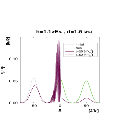
Figure 1: Snapshots of the wave function squared at various times

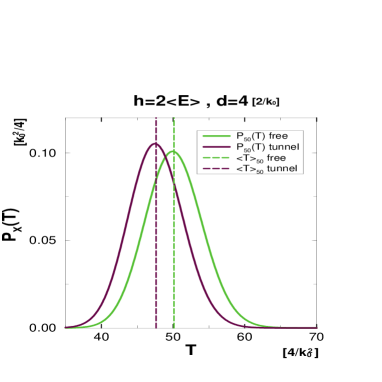
Figure 2: The arrival time distribution for detection at $X=50[2/k_{0}]$

Let us begin by watching the motion of wave packets with an $h=1.1\langle E\,\rangle$, $d=1.5$ potential. The snapshots of the motion are shown in Fig. 2, in which the free packet motion is also shown for comparison. Both packets spread due to the dispersive properties that come from their own masses. The packet moving through the potential barrier experiences reflection and transmission and the peak of the transmitted part will often advance compared to the free packet. It is usually explained that this is because the higher momentum components of the packet preferably go through the barrier and they propagate faster than the lower momentum parts due to their dispersive properties. That is, the advancement results from reshaping of the transmitted packet. However, tracing the peak of the packet is often difficult because near the barrier the peak cannot be clearly identified. Therefore we must use more well-defined quantities, $P_{X}(T)$ and $\left\langle T\right\rangle_{X}$.

Analysis 1: Detection at $X=50$

Now let us calculate $P_{X}(T)$ and $\left\langle T\right\rangle_{X}$ at $X=50$ with an $h=2\langle E\,\rangle$, $d=4$ potential. In Fig. 2, the arrival time distributions $P_{X}(T)$ are plotted for the free and tunneling particles and the mean arrival times $\left\langle T\right\rangle_{X}$ are shown by dashed lines. The remarkable feature of $P_{X}(T)$ is the stretched tail and the shift of the peak caused by spread of the packet. For the free case, $\left\langle T\right\rangle_{X}=50.13$ is later than $T=50$, which is expected from the group velocity of the free packet, and “the peak of $P_{X}(T)$” $=49.94$ is earlier than $T=50$. It is also seen that, because of the packet’s reshaping, $P_{X}(T)$ for the tunneling particle has a narrower shape than the free one and “$\left\langle T\right\rangle_{X}$ for the tunneling particle” $=47.65$ is earlier than the free one. However, it should be noted that only one detection far from the barrier cannot describe the dynamics of packets since we should discriminate effects in and out of the potential barrier. Therefore we investigate detection at various points.

Analysis 2: Detection at various points

When we try to give a definite answer to the so-called tunneling time problem, we might have to calculate the difference $\Delta=\left\langle T\right\rangle_{d}-\left\langle T\right\rangle_{0}$, since this problem demands that we answer the question “How long does it take for the particle to tunnel across the barrier?” However the difference $\Delta$ does not make much sense because, as we can see in Fig. 2, the shape of the packet is oscillating frequently at the entrance of the barrier and it is difficult to distinguish between the tunneling packet and the reflected one, that is, $\left\langle T\right\rangle_{0}$ is not a good physical quantity. On the other hand, the packet has a relatively clear shape at the exit of the barrier. Therefore we can analyze what time the packet will appear at the exit of the barrier and how it moves after that.

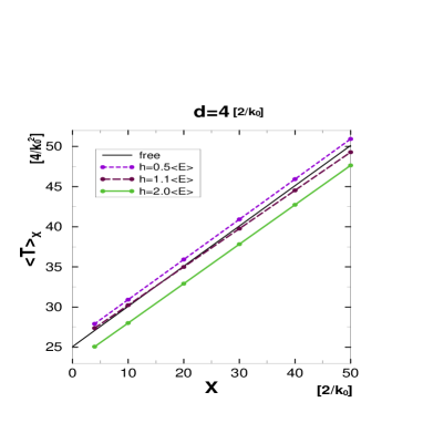
Figure 3: The mean arrival time for detection at various points

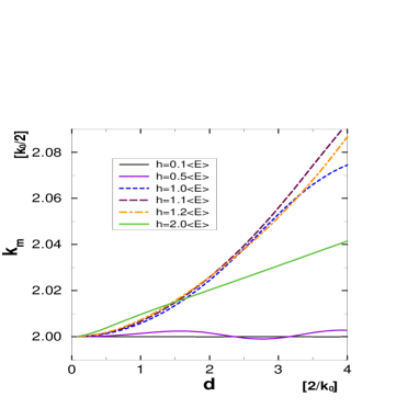
Figure 4: The mean momentum of the transmitted packet

We calculate $\left\langle T\right\rangle_{X}$ for the exit of the barrier and several points after that: $\left\langle T\right\rangle_{X}$ at $X=d,10,20,30,40,50$, with $d=4$, $h=0.5\langle E\,\rangle,1.1\langle E\,\rangle,2\langle E\,\rangle$ barrier potentials (Fig. 4). We can see two remarkable features in this figure. The first is that for high barriers $\left\langle T\right\rangle_{d}$ is earlier than in the free case, but it is later for low barriers. That is, it seems that the transmitted packet arrives at the barrier exit earlier than the free one for tunneling dominated cases. These are regarded as effects in the barrier. The second feature is that, after passing the barrier, the tunneling packet moves with a constant mean velocity larger than that of the corresponding free packet. This is an effect outside the barrier. These two types of effect are combined to cause nontrivial behaviors of the arrival time. For example, in the case of $d=4$, $h=0.5\langle E\,\rangle$, the tunneling packet arrives at the barrier exit $X=4$ later than the free packet; however, after exiting the barrier, the tunneling packet catches up with the free one and overtakes it at $X\simeq 15$. After all, it depends on $X$ which arrives at $X$ earlier, the tunneling or the free packet.

We can see the second effect clearly in the Fourier transformed form of the transmitted packet [34],

$$\psi(x,t)=(4\pi\sigma^{2})^{1/4}\int\frac{dk}{2\pi}e^{-\sigma^{2}(k-k_{0})^{2}/2}|T_{k}|e^{i\theta}e^{i[k(x-x_{0})-\omega t]},$$ (29)

where $T_{k}$ is the transmission amplitude and $\theta$ is the phase. Using an analytically obtained $|T_{k}|$, the mean momentum $k_{m}$ can be calculated for the transmitted packet. Results for several potential conditions are shown in Fig. 4. For “high” barriers, a wider barrier gives a larger mean momentum in the region $d:[0,4]$. This is because as $d$ grows the $|T_{k}|$ support shifts to the higher momentum side. Therefore the statement “Higher momentum components of the packet preferably go through the barrier” applies indeed. This kind of “acceleration” effect is found in other areas of physics [28].

Analysis 3: Detection at the barrier exit $X=d$

To see the in-barrier effects more definitely, we calculate the difference between mean arrival times for the tunneling packet and the free one at the barrier exit $X=d$,

$$\Delta T \equiv \left\langle T\right\rangle_{d}^{\rm tunnel}-\left\langle T\right\rangle_{d}^{\rm free}.$$ (30)

Results for the same potential conditions as in Fig. 4 are shown in Fig. 5. At first we see that in the small $d$ region $\Delta T$ is positive, that is, the tunneling packet gets behind the free one, for any potential height. However, as $d$ increases, $\Delta T$ shows different behaviors according to the potential height.

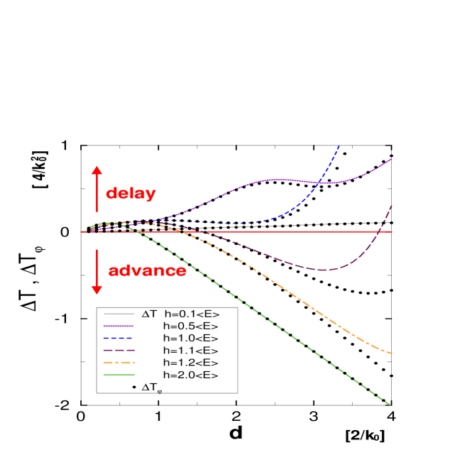
Figure 5: The difference between mean arrival times at the barrier exit $X=d$ for the tunneling packet and the free one: $\Delta T\equiv\left\langle T\right\rangle_{d}^{\rm tunnel}-\left\langle T\right\rangle_{d}^{\rm free}$. $\Delta T_{\varphi}$ (shown by dots) are the same quantity calculated by the stationary phase method for each potential.

Roughly speaking, for a “low” barrier $\Delta T$ almost stays positive but for a “high” barrier $\Delta T$ becomes negative. The “high” barrier means that the tunneling modes dominate in the transmitted packet. In the large $d$ region, $\Delta T$ is negative, that is, the tunneling packet goes ahead of the free one for the tunneling dominated case. We also see a strange behavior where $\Delta T$ changes sign twice and finally becomes positive. The typical case in Fig. 5 is the $h=1.1\langle E\,\rangle$ barrier. We understand this effect as follows. For a very wide barrier, over-the-barrier modes dominate in thetransmitted packet ($\omega_{m}=k_{m}^{2}/2>h$). That is, as in the “low” barrier case, $\Delta T$ becomes positive again.

In Fig. 5 we also plotted an analogous quantity $\Delta T_{\varphi}$ calculated by the stationary phase method. We define $\Delta T_{\varphi}$ as follows:

$$\tau_{\varphi} \equiv \left.\frac{d\theta}{d\omega}\right|_{\omega=\omega_{m}},$$ (31)

$$\Delta T_{\varphi} \equiv \left(\frac{1}{v_{g}(k_{m})}-\frac{1}{v_{g}(k_{0})}\right)(d-x_{0})+\tau_{\varphi},$$ (32)

where $\theta$ is the phase shift of the transmitted wave defined in Eq. (29) and $v_{g}(\cdot)$ are the group velocities $v_{g}(k_{m})=\left.(d\omega/dk)\right|_{k=k_{m}}=k_{m}$, $v_{g}(k_{0})=k_{0}$. In the ordinary tunneling time problem context $\tau_{\varphi}$ is called the phase time. As seen in Fig. 5, although $\Delta T_{\varphi}$ has good agreement with our $\Delta T$ in the small $d$ region, as $d$ increases, the difference becomes clear for $h\simeq\langle E\,\rangle$ barriers. This is because for such barriers the momentum distribution $e^{-\sigma^{2}(k-k_{0})^{2}/2}|T_{k}|$ is no longer symmetric with respect to $k_{m}$, and the packet’s peak given by the stationary phase method loses physical significance.

We would like to close this section by referring to the relationship between our results and the experiment by Chiao and co-workers, that is, tunneling of the massless photon. Of course our model does not describe the propagation of photons, and we now mention only the qualitative behavior. Because the energy of the photon in the vacuum is exactly proportional to its momentum, the group velocity of the photon after tunneling is constant $c$. Therefore we get an $X$ independent constant value of the difference $\Delta T=\left\langle T\right\rangle_{X}^{\rm tunnel}-\left\langle T\right\rangle_{X}^{\rm free}$ at any $X\geq d$. Since their experimental setup is the tunneling dominated one, it may correspond to our model with high and medium wide barriers. Then our results are consistent with their experimental observation that the tunneling photon arrives earlier than the free photon.

4 Nelson’s stochastic interpretation

Now we consider the stochastic interpretation of quantum mechanics introduced by Nelson. This approach interprets the motion of particles in quantum mechanics as “real-time” stochastic processes [37]. Nelson substituted the coordinate variable $x(t)$ for a stochastic variable performing the Brownian motion in a certain drift force field. The time evolution of $x(t)$ is described by the Ito-type stochastic differential equation,

$$dx(t)=b\left(x(t),t\right)dt+dw(t),$$ (33)

where $b(x,t)$ is the so-called drift term, given by the ordinary Schrödinger wave function $\psi(x,t)$ as

$$b(x,t)=\frac{\hbar}{m}\frac{\partial}{\partial x}\left({\rm Im+Re}\right){\rm ln}\psi(x,t).$$ (34)

The Gaussian noise $dw$ characterizes the stochastic behavior and should have the following statistical properties:

$$\langle dw(t)\rangle=0,\quad\langle dw(t)dw(t)\rangle=\frac{\hbar}{m}dt.$$ (35)

Starting with an initial distribution of $x(0)$ we solve Eq. (33) and obtain sample paths. Averaging a physical variable with these sample paths, we can calculate the expectation value for the ordinary probability distribution $\left|\psi(x,t)\right|^{2}$. In this approach, we are able to observe “trajectories” of real-time motion of a particle, that is, to describe the quantum mechanical time evolution by a classical stochastic process.

Thus in Nelson’s approach it may be possible to understand an imaginary-time process such as tunneling in real-time language. It was pointed out that the tunneling particle “hesitates” in front of the barrier as seen in Fig. 7 [38]. This fact was understood to imply that the particle tunneling through the barrier should always be delayed compared with the free one because of this hesitation. Is it contradictory to our results? Nelson’s approach can reproduce physical quantities in standard quantum mechanics, and there cannot be any conflict.

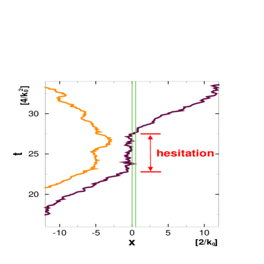
Figure 6: Typical sample paths with hesitation

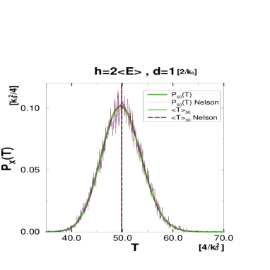
Figure 7: Comparison of two methods      

Now we analyze the mean arrival time in Nelson’s stochastic interpretation. One intuitive idea of defining the arrival time for a sample path is to measure the time for a path to reach a detecting point for the first time: “the first time counting scheme” [39]. However, this notion has no counterpart in the physical quantities of standard quantum mechanics. We have to work with the probability of existence of paths at a point (or a section) at some definite time. The difference between these two notions is that the latter counts the possibility of a path going beyond the point and coming back to it at the measuring time.

We define a probability function $\rho_{X}^{\rm N}(T)$,

$$\rho_{X}^{\rm N}(T)~{}dx=\frac{n(X,T)}{N},$$ (36)

where $N$ is the total number of sample paths and $n(X,T)$ is the number of sample paths that exist in $[X,X+dx]$ at time $T$. As stressed before, we will count the number of paths passing a target point over and over again, i.e., we now employ “the multiple counting scheme.” With this scheme, we define the arrival time distribution $P_{X}^{\rm N}(T)$ and the mean arrival time $\left\langle T\right\rangle_{X}^{\rm N}$ of the particle in Nelson’s stochastic interpretation,

$$P_{X}^{\rm N}(T)~{}dT=\frac{\rho_{X}^{\rm N}(T)~{}dT}{{\displaystyle\int_{0}^{\infty}dT\rho_{X}^{\rm N}(T)}},$$ (37)

$$\left\langle T\right\rangle_{X}^{\rm N}=\int_{0}^{\infty}TP^{\rm N}_{X}(T)dT.$$ (38)

We calculate $P_{X}^{\rm N}(T)$ and $\left\langle T\right\rangle_{X}^{\rm N}$ with an $h=2\left\langle E\right\rangle$, $d=1$ barrier by solving Eq. (33) to get $N=10^{6}$ sample paths. The result is shown in Fig. 7. The distribution $P_{X}^{\rm N}(T)$ agrees with $P_{X}(T)$ very well; therefore $\left\langle T\right\rangle_{X}^{\rm N}$ agrees with $\left\langle T\right\rangle_{X}$. The distribution given by Nelson’s approach exactly reproduces our previous results, just as expected. Of course, if we employ the first time counting scheme, $P_{X}^{\rm N}(T)$ shifts to an earlier time region and therefore $\left\langle T\right\rangle_{X}^{\rm N}$ is smaller than $\left\langle T\right\rangle_{X}$.

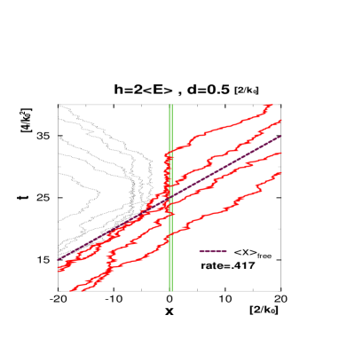
Figure 8: Sample paths for $\Delta T>0$

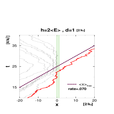
Figure 9: Sample paths for $\Delta T<0$

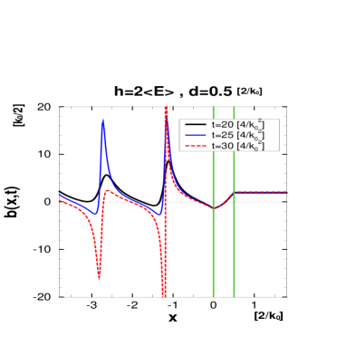
Figure 10: Drift velocity for $\Delta T>0$

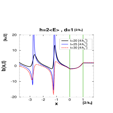
Figure 11: Drift velocity for $\Delta T<0$

Then, we should answer the paradoxical question, “Why does a hesitating particle arrive earlier than the free one?” To answer this question, let us compare the two cases of $\Delta T>0$ and $\Delta T<0$. First we show typical sample paths for two cases, $\Delta T>0~{}$($\Delta T=0.084$), $h=2\left\langle E\right\rangle$, $d=0.5$ in Fig. 9 and $\Delta T<0~{}$($\Delta T=-0.138$), $h=2\left\langle E\right\rangle$, $d=1$ in Fig. 9. In both figures we also plot the average position of the free sample paths $\left\langle x\right\rangle_{\rm free}$. We should pay attention to the point $(x,t)=(0,25)$ because $\left\langle x\right\rangle_{\rm free}$ arrives in $x=0$ at $t=25$. The two figures, Fig. 9 and Fig. 9, make a remarkable contrast. That is, although in Fig. 9 even the paths that arrive at $x=0$ later than $t=25$ can pass through the barrier, in Fig. 9 essentially only the paths that arrived at $x=0$ earlier than $t=25$ can go through it. The “hesitation” property is seen in both cases. In Fig. 9, however, even with “hesitation,” the averaged tunneling path can appear at the barrier exit $x=d$ earlier than the averaged free path because the tunneling path arrived at $x=0$ much earlier than $\left\langle x\right\rangle_{\rm free}$. This is the key to the mystery between hesitation and advancement.

Well, why do the tunneling paths conduct themselves in such a strange way? In the first place, why does hesitation occur? The reason is hidden in the time dependence of the drift velocity $b(x,t)$. We show $b(x,t)$ for the same conditions discussed above, especially near the potential barrier (Fig. 11 and Fig. 11). In the foreground of the barrier, according to the interference of the incident packet and the reflected packet, $b(x,t)$ oscillates frequently and becomes null many times. Especially near the barrier entrance $x=0$, $b(x,t)$ changes from positive to negative, where the particle is “trapped.” These effects cause the path’s hesitation.

At earlier times, $b(x,t)$ is almost always positive value but at later times, it becomes almost always negative. In Fig. 11, this tendency is extreme and realization of the tunneling path is much rarer than in Fig. 11. This is the reason why the early arrived paths tend to pass the barrier more easily. After all, there is no inconsistency between our results and the hesitation behavior in Nelson’s interpretation.

Furthermore, Nelson’s interpretation provides us an intuitive explanation of our results. Let us consider the high potential barrier case. It is important that every transmitted path hesitates to some extent. In the small $d$ region, because of the high transmission rate, even a path arriving at $x\simeq 0$ relatively late can pass the barrier, and as a result we find $\Delta T>0$. As $d$ increases, the transmission rate becomes lower and only the paths arriving at $x\simeq 0$ earlier can penetrate the barrier, and as a result we find $\Delta T<0$. Finally, as $d$ becomes very large, the paths arriving at $x\simeq 0$ very early hesitate there for a very long time; therefore $\Delta T$ becomes positive again.

Of course, we must recall that the “path” in Nelson’s view never corresponds to a real particle in ordinary quantum mechanics, and the explanation we gave above is just an interpretation. The same is true for an interpretation by the Bohm trajectory [12, 13]. It may be interesting to regard the path as a physical one and to calculate various quantities that cannot be calculated in ordinary quantum mechanics (the tunneling time $\Delta^{\rm N}=\left\langle T\right\rangle_{d}^{\rm N}-\left\langle T\right\rangle_{0}^{\rm N}$, quantities calculated in the first time counting scheme, etc.). Although these attempts may give us deeper insights into quantum dynamics, the validity and significance of them have not been argued much so far [40, 41].

5 Summary

Supposing an ideal detector, we defined simple expressions for the arrival time distribution $P_{X}$ and the mean arrival time $\left\langle T\right\rangle_{X}$, and applied them to analysis of wave packet tunneling. We defined $\Delta T\equiv\left\langle T\right\rangle_{d}^{\rm tunnel}-\left\langle T\right\rangle_{d}^{\rm free}$ and calculated it for various barrier conditions and showed the barrier effects clearly. In the small $d$ region, $\Delta T$ is always positive, but as $d$ increases, $\Delta T>0$ for the over-the-barrier case and $\Delta T<0$ for the tunneling case. After tunneling, the packet usually moves faster than the free one because it preferentially consists of the higher momentum modes of the incident packet. The barrier works as an acceleration filter in a sense. We also clarified that the stationary phase method gives a good approximation to our results, particularly in the small $d$ region.

We also confirmed that the stochastic interpretation introduced by Nelson reproduces our results. Furthermore, we clarified how the “hesitation” of the tunneling paths in Nelson’s picture is consistent with the advancement of the tunneling packet. The key observation is that the paths arriving at the barrier earlier than the free mean paths tend to penetrate the barrier more easily. We pointed out that this property can be explained by the time dependence of the drift velocity $b(x,t)$ and found that the behavior of $\Delta T$ is intuitively understandable with Nelson’s language.

References

-
[1]
Quantum Optical Studies of Tunneling and other Superluminal Phenomena
R. Y. Chiao and A. M. Steinberg, Phys. Scr. T76, 61 (1998). -
[2]
Measurement of the Single-Photon Tunneling Time
A. M. Steinberg, P. G. Kwiat, and R. Y. Chiao, Phys. Rev. Lett. 71, 708 (1993). -
[3]
An atom optics experiment to investigate faster-than-light tunneling
A. M. Steinberg, S. Myrskog, H. S. Moon, H. A. Kim, J. Fox, and J. B. Kim, Ann. Phys. (Leipzig) 7, 593 (1998). -
[4]
Light speed reduction to 17 metres per second
in an ultracold atomic gas
L. V. Hau, S. E. Harris, Z. Dutton, and C. H. Behroozi, Nature (London) 397, 594 (1999). -
[5]
Speed of light in non-trivial vacua
J. I. Latorre, P. Pascual, and R. Tarrach, Nucl. Phys. B 437, 60 (1995). -
[6]
Tests of quantum gravity from observations of -ray bursts
G. Amelino-Camelia, J. Ellis, N. E. Mavromatos, D. V. Nanopoulos, and S. Sarkar, Nature (London) 393, 763 (1998). -
[7]
Quantum Evolution in Space-Time Foam
L. J. Garay, Int. J. Mod. Phys. A 14, 4079 (1999). -
[8]
Severe Limits on Variations of the Speed of Light with Frequency
B. E. Schaefer, Phys. Rev. Lett. 82, 4964 (1999). -
[9]
Propagation of a Gaussian wave packet in an absorbing medium
M. Tanaka, M. Fujiwara, and H. Ikegami, Phys. Rev. A 34, 4851 (1986). -
[10]
Time in the Quantum Theory and the Uncertainty Relation
for Time and Energy
Y. Aharonov and D. Bohm, Phys. Rev. 122, 1649 (1961). -
[11]
Tunneling-time probability distribution
R. S. Dumont and T. L. Marchioro, Phys. Rev. A 47, 85 (1993). -
[12]
Arrival time distributions
C. R. Leavens, Phys. Lett. A 178, 27 (1993). -
[13]
Distributions of delay times and transmission times
in Bohm’s causal interpretation of quantum mechanics
W. R. McKinnon and C. R. Leavens, Phys. Rev. A 51, 2748 (1995). -
[14]
Time of Arrival in Quantum Mechanics
J. G. Muga, S. Brouard, and D. Macias, Ann. phys. (N.Y.) 240, 351 (1995). -
[15]
Time-of-arrival in quantum mechanics
N. Grot, C. Rovelli, and R. S. Tate, Phys. Rev. A 54, 4676 (1996). -
[16]
Positive-Operator-Valued Time Observable in Quantum Mechanics
R. Giannitrapani, Int. J. Theor. Phys. 36, 1575 (1997). -
[17]
Measurement of time of arrival in quantum mechanics
Y. Aharonov, J. Oppenheim, S. Popescu, B. Reznik, and W. G. Unruh, Phys. Rev. A 57, 4130 (1998). -
[18]
Space-time properties of free-motion time-of-arrival eigenfunctions
J. G. Muga, C. R. Leavens, and J. P. Palao, Phys. Rev. A 58, 4336 (1998). -
[19]
Arrival time in quantum mechanics
V. Delgado and J. G. Muga, Phys. Rev. A 56, 3425 (1997). -
[20]
The time of arrival concept in quantum mechanics
J. G. Muga, R. Sala, and J. P. Palao, Superlattices Microstruct. 23, 833 (1998). -
[21]