Nonlinear Matter Wave Dynamics with a Chaotic Potential

Abstract

We consider the case of a cubic nonlinear Schrödinger equation with an additional chaotic potential, in the sense that such a potential produces chaotic dynamics in classical mechanics. We derive and describe an appropriate semiclassical limit to such a nonlinear Schrödinger equation, using a semiclassical interpretation of the Wigner function, and relate this to the hydrodynamic limit of the Gross-Pitaevskii equation used in the context of Bose-Einstein condensation. We investigate a specific example of a Gross-Pitaevskii equation with such a chaotic potential: the one-dimensional delta-kicked harmonic oscillator, and its semiclassical limit. We explore the feasibility of experimental realization of such a system in a Bose-Einstein condensate experiment, giving a concrete proposal of how to implement such a configuration, and considering the problem of condensate depletion.

PACS numbers: 03.75.-b, 05.45.-a, 03.65.Bz, 42.50.Vk

I Introduction

Chaos in classical Hamiltonian systems, most simply thought of as the extreme sensitivity of trajectories in phase space to initial conditions, making long term predictions extremely difficult, is by now broadly understood [1, 2]. More recently, the field of quantum chaos, for our purpose meaning the study of quantum mechanical equivalents of classical chaotic systems, has been the subject of much investigation [1, 2, 3]. From this it does seem that the dynamics of quantum mechanical systems can be divided into regular and irregular subsets, with distinct differences between the two, just as is the case in classical mechanics. For example, due to the unitarity of the evolution of the state vector, there can be no equivalent of sensitivity to initial conditions in the Hilbert space, but there appears to be an equivalent sensitivity to perturbation which distinguishes quantum chaotic motion [4]. A certain amount of understanding has thus been achieved, although there are still unresolved problems, in particular how to extract classical chaos from quantum mechanics [5].

Quantum dynamics are determined by the Schrödinger equation. A seemingly natural extension is to ask what happens when we take a quantum chaotic Schrödinger equation, and add some kind of nonlinearity. This is something which has been much less studied [6], and is certainly of more than academic interest; such equations do appear in nature, for example the Gross-Pitaevskii equation in the field of Bose-Einstein condensation [7, 8], and also in the field of nonlinear optics [9]. There are thus experimentally accessible systems in which such chaotic effects may manifest themselves.

It is also interesting to note that just as in the case of quantum mechanics, where if one takes the limit $\hbar\rightarrow 0$ one expects to regain classical dynamics, one can also carry out this limit for nonlinear Schrödinger equations. This produces equations reminiscent of classical hydrodynamics, an interpretation also extensively used in the theoretical study of Bose-Einstein condensates [10]. This interconnection of different kinds of dynamics is displayed schematically in Fig. (1).

We will firstly be concerned with effective “single particle” systems. That is to say, where one takes a linear single particle Schrödinger equation with a potential which is known to produce chaotic dynamics in Hamilton’s equations of motion, and adds a nonlinearity to it. The Gross-Pitaevskii equation (for example) describes the collective dynamics of huge numbers of particles, but may nevertheless be thought of as an effective single particle wave equation. We later consider corrections to this interpretation, taking into account more fully the many body dynamics.

It is thus of general interest to determine how effects of classical chaos and quantum chaos manifest themselves in the dynamics of nonlinear Schrödinger equations, and to what extent the dynamics of the nonlinear Schrödinger equation can be explained by motion in the hydrodynamic limit, as determined by the hydrodynamic equations.

II Generalities

A Gross-Pitaevskii Equation

In this paper we will consider explicitly only one dimensional systems, although the analytic results presented can easily be generalized to two or three spatial dimensions. To simplify things further, we consider only the cubic nonlinearity explicitly, the simplest nonlinearity possible, resulting in the one dimensional Gross-Pitaevskii equation, well known in the context of Bose-Einstein condensation:

$$i\hbar\frac{\partial}{\partial t}\varphi=-\frac{\hbar^{2}}{2m}\frac{\partial^{2}}{\partial x^{2}}\varphi+V(x,t)\varphi+u|\varphi|^{2}\varphi,$$ (1)

where $\varphi(x,t)$ is the wavefunction and $u$ the strength of the nonlinearity. Again, the analytic results here can easily be generalized to more complicated nonlinearities. Such a simplified system demonstrates all the main features of a nonlinear Schrödinger equation, and is perfectly adequate for illustrative purposes. This kind of simplified system is in fact experimentally accessible, for example in a Bose-Einstein condensate experiment, as will be shown in Section VI.

B Hydrodynamic Equations

It is tempting to think of the hydrodynamic equations as the semiclassical limit of the Gross-Pitaevskii equation. This turns out to be not quite so, as will be shown in Sec. III. We nevertheless sketch out the standard derivation of the hydrodynamic equations, in order to set notation, and so that later we can point out the differences between the hydrodynamic limit and the genuine semiclassical limit, which we will derive using Wigner functions.

We rewrite the Gross-Pitaevskii equation Eq. (1) using the density $\rho$ and a momentum field $P$ [11], defined in terms of the wavefunction $\varphi=\sqrt{\rho}e^{iS/\hbar}$ as:

$$\rho = |\varphi|^{2},$$ (2)

$$\rho P = \frac{\hbar}{2i}\left[\varphi^{*}\frac{\partial}{\partial x}\varphi-\left(\frac{\partial}{\partial x}\varphi^{*}\right)\varphi\right]=\rho\frac{\partial}{\partial x}S.$$ (3)

The resulting equation of motion for the density is

$$\frac{\partial}{\partial t}\rho=-\frac{\partial}{\partial x}\left(P\rho\right).$$ (4)

Before moving to the equation of motion for $P$, we first consider the equation for $S$, which is

$$\frac{\partial}{\partial t}S=-\frac{1}{2m}\left(\frac{\partial}{\partial x}S\right)^{2}-V(x,t)-u\rho+\frac{\hbar^{2}}{2m\sqrt{\rho}}\frac{\partial^{2}}{\partial x^{2}}\sqrt{\rho}.$$ (5)

The equation of motion for the momentum field $P$ is exactly the spatial derivative of Eq. (5):

$$\frac{\partial}{\partial t}P=-\frac{\partial}{\partial x}\left[\frac{P^{2}}{2m}+V(x,t)+u\rho-\frac{\hbar^{2}}{2m\sqrt{\rho}}\frac{\partial^{2}}{\partial x^{2}}\sqrt{\rho}\right].$$ (6)

Taking the hydrodynamic limit [8, 10] consists of abandoning the term in Eq. (6) proportional to $\hbar^{2}$, generally justified by claiming that the density $\rho$ is sufficiently smooth for its derivatives to be insignificant, resulting in

$$\frac{\partial}{\partial t}P=-\frac{\partial}{\partial x}\left[\frac{P^{2}}{2m}+V(x,t)+u\rho\right].$$ (7)

Clearly, to get Eq. (7), we have discarded all quantum character of the Gross-Pitaevskii equation. Also note that if the corresponding term is abandoned in Eq. (5) in the case where $u=0$ and $V$ is time independent, we get the Hamilton-Jacobi equation for a single particle in the potential $V$, with the interpretation that $\partial S/\partial x$ is the canonically conjugate momentum to the coordinate $x$ [12].

This seems to indicate that the hydrodynamic equations Eqs. (4,7) might be an equivalent “classical” limit to the Gross-Pitaevskii equation with finite $u$ [Eq. (1)]. As previously stated however, this turns out to be not quite so, as we shall soon see.

III Wigner Function Dynamics

A Expansion in $\hbar$

We wish to carry out a consistent expansion of Eq. (1) around $\hbar$, in order to clearly separate classical from quantum dynamics, and to provide order by order corrections. We will do this by considering the dynamics of the Wigner function $W$, which is exactly equivalent to the wavefunction $\varphi$, in the sense that all information about the wavefunction is contained within its Wigner representation.

We define the Wigner function (for a pure state) as

$$W(x,p)=\frac{1}{2\pi\hbar}\int_{-\infty}^{\infty}d\tau e^{-ip\tau/\hbar}\varphi^{*}(x-\tau/2)\varphi(x+\tau/2).$$ (8)

It is well known that the dynamics of the Wigner function of a single particle to lowest order give simply the classical Liouville equation of a distribution of noninteracting particles [5]. The exact expression to all orders in $\hbar$ for the time evolution of the Wigner function $W$ is given by:

$$\frac{\partial}{\partial t}W = \sum_{s=0}^{\infty}\frac{(-1)^{s}}{(2s+1)!}\left(\frac{\hbar}{2}\right)^{2s}\frac{\partial^{2s+1}}{\partial x^{2s+1}}H\frac{\partial^{2s+1}}{\partial p^{2s+1}}W-\frac{\partial}{\partial p}H\frac{\partial}{\partial x}W$$ (9)

where $H$ is the single particle classical Hamiltonian function. How to obtain this expression is sketched in Appendix A. Setting $\hbar=0$ we see we do indeed get the classical Liouville equation

$$\frac{\partial}{\partial t}W=\frac{\partial}{\partial x}H\frac{\partial}{\partial p}W-\frac{\partial}{\partial p}H\frac{\partial}{\partial x}W,$$ (10)

so long as the initial Wigner function can in fact be interpreted as a classical probability density (i.e. is non-negative). If we have as a classical Liouville density a delta distribution, $W(x,p)=\delta(x-x_{0})\delta(p-p_{0})$, we regain classical point dynamics. One can think of a point particle being regained from quantum mechanics if we have a coherent state centred at $x=x_{0}$ and $p=p_{0}$ and let $\hbar\rightarrow 0$, causing the Wigner function to tend to just such a delta distribution.

It is worth mentioning that although we talk blithely about letting $\hbar$ tend to zero, this is in fact physically meaningless. As $\hbar$ is a constant, we must in fact expand around some scaling parameter to do with the characteristic action scales of the problem at hand, such that at some point the quantum corrections should be completely dominated, at least for some characteristic time [5]. Generally some appropriate parameter presents itself, as will be shown in the model we present in Section IV, and expansions where it is stated that the limit $\hbar\rightarrow 0$ is explored should be interpreted in this manner.

What we now wish to do is to take an equivalent limit to that presented in Eqs. (9,10) for the Gross-Pitaevskii equation, with the object of getting some kind of Liouville equation with the nonlinearity taken into account. The full expansion of the Wigner function dynamics governed by Eq. (1) in terms of $\hbar$ turns out to be:

$$\frac{\partial}{\partial t}W = -\frac{\partial}{\partial p}H\frac{\partial}{\partial x}W+\sum_{s=0}^{\infty}\frac{(-1)^{s}}{(2s+1)!}\left(\frac{\hbar}{2}\right)^{2s}\frac{\partial^{2s+1}}{\partial x^{2s+1}}\left[H+u\rho\right]\frac{\partial^{2s+1}}{\partial p^{2s+1}}W,$$ (11)

where we have the density

$$\rho(x)=\int_{-\infty}^{\infty}dp^{\prime}W(x,p^{\prime})=|\varphi(x)|^{2},$$ (12)

exactly as in the hydrodynamic equations, Eqs. (4,7). The result of Eq. (11) is outlined in Appendix A.

If we take only the zeroth term in the infinite sum, we do indeed obtain a kind of Liouville equation

$$\frac{\partial}{\partial t}W=\frac{\partial}{\partial x}H_{\rho}\frac{\partial}{\partial p}W-\frac{\partial}{\partial p}H_{\rho}\frac{\partial}{\partial x}W,$$ (13)

where

$$H_{\rho}=\frac{p^{2}}{2m}+V(x,t)+u\rho,$$ (14)

i.e. there is an additional “potential” proportional to the density of the distribution in position space. This can be interpreted as a large number of classical particles initially placed in phase space according to some kind of distribution function and interacting repulsively with one another, i.e. as a kind of non-ideal gas. If $u$ is large we would generally expect large numbers of such particles concentrated heavily in some cell in position space to tend to drive one another apart, meaning that large values of $\rho$ should in the long term be heavily disfavoured.

B Hydrodynamics Related to Wigner Function Dynamics

Hydrodynamic equations can also be derived from the equation of motion for the Wigner function Eq. (11), and if one expects the hydrodynamic equations to describe a semiclassical limit of the Gross-Pitaevskii equation, this should be consistent with the semiclassical limit described by the Liouville-like equation of Eq. (13). In this section we conclusively show this not to be the case, and explain why this is so.

In terms of the Wigner function, $P$ is defined by:

$$\rho(x)P(x)=\int_{-\infty}^{\infty}dppW(x,p),$$ (15)

where $\rho(x)$ has already been defined by Eq. (12). $P$ is thus seen to be simply the first order momentum moment of the Wigner function. It turns out to be useful to define higher order moments as well:

$$\rho(x)P_{n}(x)=\int_{-\infty}^{\infty}dpp^{n}W(x,p).$$ (16)

The derivation of the equation of motion for $\rho$ is carried out in Appendix B, and is exactly the continuity equation of Eq. (4), correct to all orders in $\hbar$. The equation of motion for $P$, again to all orders in $\hbar$, turns out to be

$$\frac{\partial}{\partial t}P = -\frac{\partial}{\partial x}[V(x,t)+u\rho]-\frac{1}{\rho m}P_{2}(x)+\frac{P}{\rho m}\frac{\partial}{\partial x}(\rho P)$$ (17)

$$= -\frac{\partial}{\partial x}\left[V(x,t)+u\rho+\frac{P_{2}}{2m}\right]-\frac{1}{\rho m}\frac{\partial}{\partial x}(\sigma_{p}^{2}\rho),$$ (18)

where $\sigma_{p}^{2}(x)=P_{2}(x)-P(x)^{2}$ is the variance of the Wigner function in $p$ at a given point in $x$.

Except for the term involving $\sigma_{p}^{2}$, Eq. (18) is identical to the hydrodynamic equation Eq. (7). However, it can be seen that Eqs. (4,18) do not form a closed system, as the equation of motion for $P(x)$ refers to the higher order moment $P_{2}(x)$. There is in fact, as shown in Appendix B, an infinite chain of differential equations for the moments $P_{n}(x)$ [13]:

$$\frac{\partial}{\partial t}P_{n}(x) = \frac{P_{n}(x)}{\rho}\frac{\partial}{\partial x}[\rho P(x)]-\frac{1}{\rho m}\frac{\partial}{\partial x}[\rho P_{n+1}(x)]-nP_{n-1}(x)\frac{\partial}{\partial x}[V(x,t)+u\rho]$$ (20)

$$-\sum_{s=1}^{n-1}\left\{\frac{(\hbar/2)^{2s}n!}{(2s+1)![n-(s+1)]!}P_{n-(s+1)}(x)\frac{\partial^{2s+1}}{\partial x^{2s+1}}[V(x,t)+u\rho]\right\}.$$

In each equation the quantum corrections are described by the sum, but there is also an infinite chain of classical corrections; the second term of Eq. (20) refers to the higher order moment $P_{n+1}(x)$. To get the second hydrodynamic equations, Eq. (7), in closed form from Eq. (18), we must additionally make the zeroth order moment approximation,

$$P_{n}(x)=P(x)^{n}.$$ (21)

In Appendix B this is treated in a little more detail.

In order to reach the “hydrodynamic limit”, it is necessary to kill off all the quantum corrections, but there is in fact a much more drastic approximation than only taking the limit $\hbar\rightarrow 0$, as a whole chain of classical corrections must be abandoned at the same time. The reason for the failure of the hydrodynamic equations as a semiclassical limit can be seen by examining our initial reasoning more closely. This was based partly on a correspondence between the hydrodynamic limit of the linear Schrödinger equation and the equivalent Hamilton-Jacobi equation, however this also implicitly assumes that the interpretation of the quantum wavefunction tends to a classical point. The Liouville dynamics given by Eqs. (10,13) describe the motion of classical distributions. As has already been mentioned, in the case of no nonlinearity ($u=0$) one can connect the two classical cases by considering a distribution of the form $W=\delta(x-x_{0})\delta(p-p_{0})$, but when one is considering a case where the dynamics are influenced by the density in position space $\rho$, this is clearly meaningless.

The correct semiclassical limit described in terms of moment equations is thus described by the following system:

$$\frac{\partial}{\partial t}\rho = -\frac{1}{m}\frac{\partial}{\partial x}[\rho P(x)],$$ (22)

$$\frac{\partial}{\partial t}P_{n}(x) = \frac{P_{n}(x)}{\rho}\frac{\partial}{\partial x}[\rho P(x)]-\frac{1}{\rho m}\frac{\partial}{\partial x}[\rho P_{n+1}(x)]-nP_{n-1}(x)\frac{\partial}{\partial x}[V(x,t)+u\rho],$$ (23)

where we must include every value of $n$. All of this is accounted for in Eq. (13). It seems clear that Eq. (13) is a simpler way of describing the correct classical limit, and is almost certainly easier to integrate numerically.

The purpose of comparing a nonlinear Schrödinger equation with its semiclassical limit is that it explicitly removes the wave-like or quantum behaviour, allowing us to see what there is that is specifically “quantum” about the dynamics of the nonlinear Schrödinger equation under consideration.

IV Model

A The Delta-Kicked Harmonic Oscillator

To gain insight into the general problem, it is useful to take a simple test system, which is (a) accessible experimentally, and (b) amenable to numerical attack. The system chosen is the one dimensional delta-kicked harmonic oscillator, which has been studied both classically [14, 15, 16, 17] and quantum mechanically [18, 19, 20, 21]. The total potential for the classical Hamiltonian consists of a standard harmonic potential perturbed by a time dependent kicking potential:

$$V(x,t)=\frac{m\omega^{2}x^{2}}{2}+K\cos(kx)\sum_{n=-\infty}^{\infty}\delta(t-n\tau),$$ (24)

where $x$ is the position, $m$ is the particle mass, $\omega$ the harmonic frequency, $K$ the kick strength, $k$ the wavenumber, and $\tau$ the time interval between kicks.

B Scaling

In our model, there are two basic parameters: the kick strength $K$, and the strength of the nonlinearity $u$. Additionally there is $\hbar$, which we have expanded around in Section III. The parameters $K$ and $u$ need to be rescaled so that they remain equivalent in different regimes, as determined by a scaling parameter which takes the place of $\hbar$. In the case of the delta-kicked harmonic oscillator there is a natural dimensionless scaling parameter, which is $\eta$, the Lamb-Dicke parameter.

$$\eta=k\sqrt{\frac{\hbar}{2m\omega}}$$ (25)

It should also be pointed out that $\eta$ is a real physical magnitude, which really can be adjusted in the laboratory, unlike $\hbar$. We call the dimensionless kicking strength $\kappa$, and the dimensionless nonlinearity strength $\upsilon$:

$$\kappa = \frac{Kk^{2}}{\sqrt{2}m\omega^{2}},$$ (26)

$$\upsilon = \frac{uk^{3}}{2\sqrt{2}m\omega^{2}}.$$ (27)

It is shown in Appendix C that $\kappa$ and $\upsilon$ have an equivalent effect on the overall dynamics for any value of $\eta$.

If, as is often the case when the trapping potential is harmonic, the Gross-Pitaevskii equation has been rescaled in terms of harmonic coordinates $(\hat{x}_{h}=\sqrt{m\omega/\hbar}\hat{x}$, $\hat{p}_{h}=\hat{p}/\sqrt{m\hbar\omega})$, then it can be written in terms of these dimensionless parameters as:

$$i\frac{\partial}{\partial t_{h}}\varphi = -\frac{1}{2}\frac{\partial^{2}}{\partial x_{h}^{2}}\varphi+V(x_{h},t_{h})\varphi+\frac{\upsilon}{\eta^{3}}|\varphi|^{2}\varphi,$$ (28)

$$V(x_{h},t_{h}) = \frac{x_{h}^{2}}{2}+\frac{\kappa}{\sqrt{2}\eta^{2}}\cos(\sqrt{2}\eta x)\sum_{n=-\infty}^{\infty}\delta(t_{h}-n\tau_{h}).$$ (29)

The wavefunctions have been rescaled so that they are properly normalized with respect to the harmonic position coordinate, and the time evolution is with respect to the dimensionless time $t_{h}=\omega t$. It is this form of the Gross-Pitaevskii equation that we use in our numerical simulations.

V Model Phase Space Dynamics

A Classical Point Dynamics

The dynamics of a classical point particle in a delta-kicked harmonic potential have been described fairly extensively elsewhere [14, 15, 16, 17]. Briefly, we choose a value for $\tau_{h}$. For a given $\tau$ there is only one free parameter which affects the phase space dynamics: $\kappa$. There is a resonance condition $\tau_{h}=2\pi r/q$ ($r/q$ is a positive rational, where $q>2$), whereby there are interconnecting channels of chaotic dynamics in the phase space [16, 17], the thickness of which depends on the kick strength $\kappa$ [16]. For $\kappa$ not too large, these form an Arnol’d stochastic web which spreads through all of phase space, and has a characteristic $q$ symmetry. For large $\kappa$, one observes global chaos. Note that Arnol’d diffusion [22] can occur in systems of less than two dimensions when the conditions for the KAM (Kolmogorov, Arnol’d, Moser) theorem [1, 23] are not fulfilled, as is the case here [15, 16, 17].

Here [and also in the following numerical work on the Gross-Pitaevskii equation Eq. (1) and Liouville equation Eq. (13)] we consider the case where $\tau_{h}=2\pi/6$ and $\kappa=1$. The scaled position and momentum are defined as

$$\tilde{x} = \frac{kx}{\sqrt{2}}=\eta x_{h},$$ (30)

$$\tilde{p} = \frac{kp}{\sqrt{2}m\omega}=\eta p_{h}.$$ (31)

These scaled variables are chosen so that the phase space dynamics of a classical point particle described in terms of them are affected only by $\kappa$ and $\tau_{h}$. As can be seen, they correspond exactly to the scaled harmonic position and momentum when $\eta=1$.

It can be seen in Fig. 2 that the phase space, in this case having a 6 symmetry, consists of a stochastic web of chaotic dynamics, where an initial condition can spread throughout phase space, enclosing cells of stable dynamics. An trajectory initially inside one of these stable cells will generally be held in a ring of six cells, equidistant from the centre, for all time (with the exception of the particle initially in the central cell, where it stays) [14].

B Gross-Pitaevskii Equation

In this section and in Sec. V C, we always work with the harmonically scaled position $x_{h}$ and momentum $p_{h}$ and with the dimensionless time $t_{h}$. For the sake of brevity we omit the $h$ subscript, and thus write these variables simply as $x$, $p$, and $t$ (or $\tau$).

We integrate numerically, using a split operator method, the Gross-Pitaevskii equation as given in Eq. (28) considering only the harmonic potential for periods of time of length $\tau$, punctuated by the exact mapping

$$\varphi(x,t^{+})=e^{-i\kappa\cos(\sqrt{2}\eta x)/\sqrt{2}\eta^{2}}\varphi(x,t^{-})$$ (32)

which accounts for the effect of the instantaneous delta kicks. This was carried out for various values of $\upsilon$ and $\eta$, where $\kappa=1$ and $\tau=2\pi/6$ in every case.

We have calculated the time averaged Wigner function, by which we mean the average of all the Wigner functions determined just before each delta kick, for 100 kick periods. The initial wavefunctions are displaced ground states. That is, the ground state of the Gross-Pitaevskii equation is determined numerically, for each value of $\upsilon$. We then locate the centre of the wavefunction at a point which is in a regular or chaotic region of the the classical single particle phase space. “Unstable” initial wave-packets are centred at $x=\sqrt{2}\pi/\eta$ (harmonic units), and “stable” initial wave-packets at $x=2\sqrt{2}\pi/\eta$. The initial wavefunctions are thus centred exactly either in the middle of a cell in phase space, or in an area dominated by web dynamics. These displaced states are the natural equivalent of coherent states for a cubic nonlinear Schrödinger equation. Just like coherent states, the density profile keeps its shape in a simple harmonic potential as it oscillates back and forth. This oscillating excitation is the so-called Kohn mode [24].

Firstly we show, in Fig. (3), the case of no nonlinearity, for the sake of reference. In this case the initial conditions are simply coherent states. Note that because it is possible for the Wigner function to have negative values, the colour representing zero is in general different in each pseudocolour plot. Thus, in each plot there is a “background” colour, which represents zero, with a superimposed pattern made up of darker and lighter shades. Notice that for $\eta=1$, the unstable initial condition [Fig. 3(a)] appears to move through phase space following the stochastic web, whereas the stable initial condition [Fig. 3(b)] simply circles around phase space, as would an initial coherent state in a simple harmonic potential. The wavefunction is clearly somewhat deformed (in the case of a harmonic potential we would see perfect circles) but is otherwise well localized and well behaved. In the case of $\eta=2$, one might be forgiven for thinking that whether the initial condition is ostensibly stable or not is of negligible importance. The fact that $\eta$ is larger has the effect that the phase space is smaller compared to the size of the initial wavefunction (as plotted here, using harmonic units), and also quantum corrections play a bigger role (see Appendix C), leading to the “tunneling” seen in Fig. 3(d), through classically forbidden areas of phase space. This tunneling can take place because the eigenstates of the Floquet operator $\hat{F}$ describing the period from just before one kick to just before the next,

$$\hat{F}=e^{-i(\hat{x}^{2}+\hat{p}^{2})\tau/2}e^{-i\kappa\cos(\sqrt{2}\eta\hat{x})/\sqrt{2}\eta^{2}},$$ (33)

are highly delocalized [18, 19, 20], as is described in Appendix D.

In Fig. 4 equivalent plots are shown when a nonlinearity of $\upsilon=0.1$ is added to the Gross-Pitaevskii equation. It can be seen that this does not make very much difference to the phase space dynamics compared to no nonlinearity (Fig. 3), which is not really unexpected.

When, as shown in Fig. 5, a nonlinearity of $\upsilon=1$ is added to the Gross-Pitaevskii equation, it can be seen that this does make a difference. Intriguingly, given that the interaction potential is more strongly repulsive, the phase space dynamics appear to be more strongly localized. In the case of an unstable initial condition [Fig. 5(a] and 5(c)] the web structure is noticeably reduced, and whereas in Fig. 4(d) there was significant tunneling leading to a very delocalized phase space distribution, in Fig. 5(d) this has effectively disappeared.

In Fig. 6, where $\upsilon=10$, this is even more marked. Where $\eta=1$, in the case of an unstable initial condition [Fig. 6(a)], density seems to be concentrated around a “ring” in phase space, based around how far out in phase space the initial condition was. Where $\eta=2$ [Fig. 6(c,d)], whether the initial condition is ostensibly stable or unstable, we see only six symmetrically placed round blobs of density, analogous to a coherent state in a harmonic potential.

C Liouville Equation

Here we wish to investigate the semiclassical limit of the dynamics of the Gross-Pitaevskii equation with a delta-kicked harmonic oscillator potential [Eq. (28)]. The appropriate dynamics are described in general by Eq. (13). As with the Gross-Pitaevskii equation, in our case this can be carried out by considering only the harmonic potential for periods of time $\tau$, punctuated by an exact map describing the momentum kick.

Equation (13) can be qualitatively determined numerically by taking an ensemble of starting points from some desired distribution, using Hamilton’s equations of motion to determine the trajectories, and using the numerically determined coarse-grained density for the overall potential governing the motion of the individual points. Obviously the coarse-grained density must be determined sufficiently frequently so that between times when it is determined, it does not change enough to have a very significant effect on the dynamics. This is in some sense analogous to the split-step method we have used to integrate the nonlinear Schrödinger equation, where as the time steps shrink to length zero, the approximate solution converges (in principle) to the exact solution.

In each case the initial distribution is chosen by determining the ground state of the harmonic potential Gross-Pitaevskii equation (for appropriate $\upsilon$ and $\eta$), shifting it so that the centre of the wavefunction is at an unstable or stable fixed point (in the classical, single particle sense), calculating the Wigner function, and interpreting this as a classical probability distribution in $x$ and $p$. The ground state Wigner function in the case of a harmonic potential is always strictly nonnegative, so one can always do this.

Note that although $\eta$ does not enter into the dynamics of Eq. (13) directly, by the above recipe it does enter by way of the choice of the initial condition, which affects the effective potential due to the distribution’s density in position space, and so on. The time averaged density distribution plots in Figs. 7–9 are chosen to have initial conditions and scaling exactly equivalent to the time-averaged Wigner function plots shown in Figs. 4–6.

In Fig. 7 we see the density distribution averaged over 100 kicks for the case where $\upsilon=0.1$. The dynamics are essentially similar to those show in Fig. 2 for various single trajectories, and we observe a much lesser degree of distribution through phase space when compared to the full Gross-Pitaevskii equation (see Fig. 4). In particular we see no tunneling in Fig. 7(d), compared to Fig. 4(d). The dynamics in the cases of “unstable” initial conditions perhaps do not appear to be very strongly chaotic. Remember that only 100 kicks have been applied, and that in the case of the single particle classical delta-kicked harmonic oscillator, there are slow chaotic dynamics along the stochastic web [14, 15, 16], with an overall tendency to diffuse “outwards” in phase space. We have examined the case of 100 kicks only in order to directly compare with the the numerically determined Gross-Pitaevskii dynamics.

If we examine Fig. 8, which shows analogous dynamics to Fig. 7 for the case that $\upsilon=1$, we observe some increased spreading out through phase space, still contained within the characteristic cells formed by the stochastic web in the case of the stable initial condition for $\eta=1$. In the case of $\eta=2$ The initial distribution seems too large for the cells, and even in the stable case there is some diffusion outwards through phase space.

Finally we consider the case where $\upsilon=10$, shown in Fig. 9. There is significant additional diffusion through phase space for the unstable initial condition, compared to the cases of $\upsilon=0.1$ (Fig. 7) and $\upsilon=1$ (Fig. 8). Even for the supposedly stable initial condition there is some density which has found its way onto the stochastic web, and appears to be diffusing outward. Nevertheless, the basic structure of the single particle stochastic web appears to be retained.

There thus appears to be a clear trend, where the larger the interaction parameter $\upsilon$, the greater the degree of diffusion outward through phase space, but nevertheless along routes typical for single particle dynamics. This has a simple explanation: when $\upsilon$ is large and the distribution is highly localized, the distribution tends to push itself apart. After this initial explosion through phase space (actively encouraged in the unstable parts of phase space) the contribution by the density to the effective potential is small, and so the by now thinly spread distribution undergoes local dynamics equivalent to single noninteracting classical particles, chaotic or stable, depending on the location in phase space.

D Interpretation

1 Overview

The most interesting thing shown by these numerical experiments, is the conclusive demonstration that the localization observed in Figs. 5, 6 is due to interference effects, caused by terms of higher order in $\hbar$ in Eq. (11) (or more correctly, higher order in $\eta^{2}$, as shown in Appendix. C). The intuitive picture of a stronger repulsive interaction driving the Wigner function/Liouville distribution apart, is fulfilled in the semiclassical limit, but breaks down when all “quantum” corrections are accounted for.

The increasing degree of localization shown with increasing $\upsilon$ in the Gross-Pitaevskii dynamics can also be qualitatively explained. As is shown in Appendix D, in the case of linear Schrödinger equation dynamics, the Floquet eigenstates are highly delocalized, due to extra symmetries connected to the fact that the wavefunction is kicked exactly six times per oscillation period. The presence of delocalized eigenstates means that the wavefunction tends to spread throughout phase space with ease; along the stochastic web if the initial condition is in a classically unstable part of phase space, and possibly by tunneling from cell to cell (promoted by large $\eta$) if the wavefunction is initially in a stable part of phase space. With increasing $\upsilon$ this symmetry is more and more perturbed, to a point where this ability to spread freely through phase space is lost. Interference effects due to higher order terms of the density in Eq. (11), act to hold the wavefunction together, in contrast to the Liouville type dynamics described by Eq. (13).

2 Density in Position Space

On this note it is instructive to look at the kinds of densities actually produced. We consider the final wavefunction, produced after 100 kicks, at a time just before a hypothetical 101st kick. In Fig. 10 we see plots of $|\varphi(x)|^{2}$ for the case $\upsilon=0.1$. Unsurprisingly for the unstable cases, and also for the stable case where $\eta=2$, the states are highly delocalized in position space, with a great deal of fine structure. In Fig. 11, this has substantially changed; the densities which were very complex are now much simplified, and even the stable initial condition for $\eta=1$ appears to have less structure when $\upsilon=1$ compared to $\upsilon=0.1$. When $\upsilon$ is increased to 10, as shown in Fig. 12, there is still some structure to the densities where $\eta=1$, wheras in the case where $\eta=2$ there appears now to be none.

Obviously much more radical change is induced for the case of $\eta=2$ when increasing $\upsilon$. Bearing in mind that $\eta^{2}$ is our effective $\hbar$, it is clear from Eq. (11) that higher order derivatives in the effective potential $V(x,t)+u\rho(x)$ will be more strongly emphasized (see also Appendix C). Between kicks, the non-Liouville corrections are due only to $\rho(x)$, as the derivatives of $x^{2}$ vanish.

Considering the cases of Figs. 12(a) and 12(b) in particular, one might ask what there is about these densities which seemingly so totally dominates the dynamics. We consider the initial state, which is simply a shifted ground state. The ground state of the Gross-Pitaevskii equation lie somewhere between the cases of a Gaussian (no nonlinearity) and the Thomas-Fermi limit [8], which is essentially an inverted parabola (large nonlinearity). With regard to the parameters we have chosen to use, the degree of “Thomas-Fermi-ness” is proportional to $\upsilon/\eta^{3}$. In the Thomas-Fermi limit, there are no higher order derivatives of $\rho$. A Gaussian however, has an infinite number of derivatives. For Figs. 12(a,b), $\upsilon/\eta^{3}=1.25$ only. The initial state density is thus more Gaussian than Paraboloid, and the large value of the effective $\hbar$ ensures that corrections due to the inevitable higher order derivatives are substantial.

Briefly: the application of a kick scrambles the phase of the position representation of a wavefunction; instantaneously the density in position space is unaffected however. When looking at Eq. (11) we see that corrections due to higher order derivatives of $\rho$ will be emphasized for larger effective $\hbar$, in our case $\eta^{2}$. The effect of these corrections appears to be a strong tendency for the shape of the wavefunction to be preserved.

In this work, we have not really explored the regime of very large nonlinearities. In view of the fact that in the Thomas-Fermi limit for the ground state there are no corrections to the Liouville-like equation of Eq. (13), it is possible that the kind of very pronounced localization observed for the case of $\eta=2$ might again be suppressed for much larger $\upsilon$.

3 Density in Momentum Space

For the sake of comparison, in Figs. (13,14,15) we show the corresponding momentum densities to the position densities of Figs. (10,11,12). The densities in position and momentum space essentially correspond, in that complex structure in one indicates complex structure in the other. This is not surprising, if we consider the kinds of Wigner functions displayed in Figs. (4,5,6).

VI Physical Model: Driven Bose-Einstein Condensate

A Introduction

A series of pioneering experiments investigating quantum chaos with atom-optical systems has been carried out by Raizen and co-workers [25], mainly for a quantum realization of the delta-kicked rotor. We take a similar approach; a possible physical realization of the delta-kicked harmonic oscillator, consisting of a single trapped ion periodically driven by a laser, has been described in [26]. This can in principle be readily extended to a periodically driven Bose-Einstein condensate.

B Single Particle

We begin by regarding a single two level atom. In the $x$ direction, it is trapped in a harmonic potential of frequency $\omega$, and driven time dependently by a laser field of Rabi frequency $\Omega(t)$, wavenumber $k$, and frequency $\omega_{L}$. We disregard motional degrees of freedom in the $y$ and $z$ directions as being presently uninteresting, and arrive at the following Hamiltonian operator:

$$\hat{H} = \frac{\hat{p}^{2}}{2m}+\frac{m\omega^{2}\hat{x}^{2}}{2}+\frac{\hbar}{2}\{\omega_{0}(|e\rangle\langle e|-|g\rangle\langle g|)+\cos(k\hat{x})[\Omega(t)e^{-i\omega_{L}t}|e\rangle\langle g|+\mbox{H.c.}]\}.$$ (34)

In a rotating frame defined by

$$\hat{U}=\exp[-i\omega_{L}t(|e\rangle\langle e|-|g\rangle\langle g|)/2],$$ (35)

and in the limit of large detuning $|\Delta|=|\omega_{L}-\omega_{0}|\gg|\Omega(t)|$, $|e\rangle$ can be adiabatically eliminated to give, after transformation to an appropriate rotating frame,

$$\hat{H}=\frac{\hat{p}^{2}}{2m}+\frac{m\omega^{2}\hat{x}^{2}}{2}+\frac{\hbar}{2}\frac{\Omega(t)^{2}}{4\Delta}[\cos(2k\hat{x})+1]|g\rangle\langle g|.$$ (36)

The laser is periodically switched on and off, giving a series of short pulses, approximated by Gaussians:

$$\Omega(t)^{2}=\Omega^{2}\sum_{n=-\infty}^{\infty}e^{-(t-n\tau)^{2}/\sigma^{2}},$$ (37)

which approximate a series of delta kicks in the limit $\sigma\rightarrow 0$. Note also that we require $\sigma\gg 1/\Delta$, otherwise the laser is too spectrally broad. Thus, we have finally

$$\hat{H} = \frac{\hat{p}^{2}}{2m}+\frac{m\omega^{2}\hat{x}^{2}}{2}+\frac{\hbar\sigma\sqrt{\pi}\Omega^{2}}{8\Delta}[\cos(2k\hat{x})+1]|g\rangle\langle g|\sum_{n=-\infty}^{\infty}\delta(t-n\tau).$$ (38)

Because we assume that the atom is always in electronic state $|g\rangle$, the $|g\rangle\langle g|$ operator can be effectively abandoned. The extra $+1$ simply adds a global phase, which can easily be accounted for, and so this can be further simplified to:

$$\hat{H} = \frac{\hat{p}^{2}}{2m}+\frac{m\omega^{2}\hat{x}^{2}}{2}+\frac{\hbar\sigma\sqrt{\pi}\Omega^{2}}{8\Delta}\cos(2k\hat{x})\sum_{n=-\infty}^{\infty}\delta(t-n\tau).$$ (39)

This is exactly the Hamiltonian for the quantum delta-kicked Harmonic oscillator, except that we have $\cos(2k\hat{x})$ instead of $\cos(k\hat{x})$. As far as scaling is concerned, this means we must in turn consider $\eta^{\prime}=2\eta$ instead of $\eta$ as the appropriate dimensionless parameter.

C Many Particles

It is clear that if we consider a many particle system, then the above derivation is independent of any particle-particle interactions which do not change the internal states of the atoms. We thus consider the model Hamiltonian of a weakly interacting Bose gas, in second quantized form:

$$\hat{H}=\int_{-\infty}^{\infty}d\vec{x}\hat{\Psi}^{\dagger}(\vec{x})\left[-\frac{\hbar^{2}}{2m}\nabla^{2}+V(\vec{x},t)+\frac{g}{2}\hat{\Psi}^{\dagger}(\vec{x})\hat{\Psi}(\vec{x})\right]\hat{\Psi}(\vec{x}),$$ (40)

where $\hat{\Psi}$ is the particle field operator, $g=4\pi\hbar^{2}a_{s}/m$, and $a_{s}$ is the $s$-wave scattering length. We take $V(\vec{x},t)$ to be

$$V(\vec{x},t)=V(x,t)+\frac{m\omega_{r}^{2}}{2}(y^{2}+z^{2}),$$ (41)

where the potential in the $x$ direction is exactly that derived above, i.e.

$$V(x,t)=\frac{m\omega^{2}x^{2}}{2}+\frac{\hbar\sigma\sqrt{\pi}\Omega^{2}}{8\Delta}\cos(2kx)\sum_{n=-\infty}^{\infty}\delta(t-n\tau).$$ (42)

We assume the radial frequency $\omega_{r}$ to be very large compared to the axial frequency $\omega$ (cigar shaped trapping configuration), and thus assume that every particle is in the harmonic oscillator ground state in $y$ and $z$. With this assumption we can integrate over $y$ and $z$, reducing to a single dimension:

$$\hat{H}=\int_{-\infty}^{\infty}dx\hat{\Psi}^{\dagger}(x)\left[-\frac{\hbar^{2}}{2m}\frac{\partial^{2}}{\partial x^{2}}+V(x,t)+\frac{g_{1d}}{2}\hat{\Psi}^{\dagger}(x)\hat{\Psi}(x)\right]\hat{\Psi}(x),$$ (43)

where $g_{1d}=m\omega g/2\pi\hbar=2\hbar\omega_{r}a_{s}$.

D Asymptotic Expansion

Using the particle number conserving formalism of Castin and Dum [27], we split the field operator $\hat{\Psi}$ of the many particle system into a condensate part and a non-condensate part:

$$\hat{\Psi}(x,t)=\varphi_{\mbox{ex}}(x,t)\hat{a}_{\varphi_{\mbox{ex}}}(t)+\delta\hat{\Psi}(x,t),$$ (44)

where $\varphi_{\mbox{ex}}$ is the exact condensate wave function, and $\delta\hat{\Psi}$ describes the non-condensate particles. Introducing the operator

$$\hat{\Lambda}_{\mbox{ex}}(x,t)=\frac{1}{\sqrt{\hat{N}}}\hat{a}_{\varphi_{\mbox{ex}}}^{\dagger}(t)\delta\hat{\Psi}(x,t),$$ (45)

it is possible to make asymptotic expansions of $\hat{\Lambda}_{\mbox{ex}}(x,t)$, $\varphi_{\mbox{ex}}(x,t)$, such that

$$\hat{\Lambda}_{\mbox{ex}} = \hat{\Lambda}+\frac{1}{\sqrt{\hat{N}}}\hat{\Lambda}^{(1)}+\frac{1}{\hat{N}}\hat{\Lambda}^{(2)}+\cdots,$$ (46)

$$\varphi_{\mbox{ex}} = \varphi+\frac{1}{\sqrt{\hat{N}}}\varphi^{(1)}+\frac{1}{\hat{N}}\varphi^{(2)}+\cdots,$$ (47)

where $\hat{N}$ is the total particle number operator.

Thus, to lowest order, the condensate particles are described by $\varphi(x)$. The time evolution of this can be shown to be given by the Gross-Pitaevskii equation [27], which in our case is

$$i\hbar\frac{\partial}{\partial t}\varphi=-\frac{\hbar^{2}}{2m}\frac{\partial^{2}}{\partial x^{2}}\varphi+V(x,t)\varphi+Ng_{1d}|\varphi|^{2}\varphi,$$ (48)

where $N$ is the total number of particles. In turn, the non-condensate particles are described to lowest order by $\hat{\Lambda}(x,t)$.

The Gross-Pitaevskii equation which we have arrived at in Eq. (48) can be rewritten in terms of the dimensionless parameters $\eta^{\prime}$, $\kappa$, and $\upsilon$, as described in Sec. IV B, where

$$\eta^{\prime} = k\sqrt{\frac{2\hbar}{m\omega}},$$ (49)

$$\kappa = \frac{\hbar k^{2}\sigma\sqrt{\pi/2}\Omega^{2}}{2m\omega\Delta},$$ (50)

$$\upsilon = \frac{8\hbar Nk^{3}\omega_{r}a_{s}}{\sqrt{2}m\omega^{2}}.$$ (51)

E Non-Condensate Particles

The mean number of the non-condensate particles is given by $\langle\delta\hat{N}\rangle=\langle\delta\hat{\Psi}^{\dagger}\delta\hat{\Psi}\rangle$, which to lowest order may be described by $\langle\hat{\Lambda}^{\dagger}\hat{\Lambda}\rangle$. In turn, $\hat{\Lambda}^{\dagger}$ and $\hat{\Lambda}$ can be expanded as

$$\left(\begin{array}[]{c}\hat{\Lambda}(x,t)\\ \hat{\Lambda}^{\dagger}(x,t)\end{array}\right)=\sum_{k=1}^{\infty}\hat{b}_{k}\left(\begin{array}[]{c}u_{k}(x,t)\\ v_{k}(x,t)\end{array}\right)+\sum_{k=1}^{\infty}\hat{b}_{k}^{\dagger}\left(\begin{array}[]{c}v_{k}^{*}(x,t)\\ u_{k}^{*}(x,t)\end{array}\right).$$ (52)

which gives rise to the following equation describing the mean number of non-condensate particles to lowest order in the perturbation expansion:

$$\langle\delta\hat{N}(t)\rangle=\sum_{k=1}^{\infty}\langle\hat{b}_{k}^{\dagger}\hat{b}_{k}\rangle\langle u_{k}(t)|u_{k}(t)\rangle+\langle\hat{b}_{k}^{\dagger}\hat{b}_{k}+1\rangle\langle v_{k}(t)|v_{k}(t)\rangle.$$ (53)

The $\hat{b}_{k}$ are time-independent [27]. We see that the time-dependence of Eq. (53) is thus contained completely within $\langle u_{k}|u_{k}\rangle$, $\langle v_{k}|v_{k}\rangle$. A system initially prepared at temperature $T$ has $\langle b_{k}^{\dagger}b_{k}\rangle=[\exp(E_{k}/k_{B}T)]^{-1}$, and so, if we take the limit $T\rightarrow 0$, we get

$$\langle\delta\hat{N}(t)\rangle=\sum_{k=1}^{\infty}\langle v_{k}(t)|v_{k}(t)\rangle.$$ (54)

We thus wish to study the dynamics of $|v_{k}(t)\rangle$ to get some idea of the change in the number of non-condensate particles, in an analogous fashion to the work of Castin and Dum when investigating the behaviour of a condensate held in a time dependent isotropic harmonic potential [28]. Note that because the Gross-Pitaevskii equation is nonlinear, it is possible to have chaos in the sense of exponential sensitivity to initial conditions within the Hilbert space. If this is the case, the above estimate of $\langle\delta\hat{N}(t)\rangle$ will grow automatically, due to the fact that this estimate is essentially from a linearization around the Gross-Pitaevskii solution [28]. Thus the rate of growth of this estimate of $\langle\delta\hat{N}(t)\rangle$ is similar to the Lyapunov exponent for the divergence of trajectories in phase space for discrete classical systems.

The dynamics of the $|u_{k}(t)\rangle$ and $|v_{k}(t)\rangle$ are given by

$$i\hbar\frac{d}{dt}\left(\begin{array}[]{c}|u_{k}(t)\rangle\\ |v_{k}(t)\rangle\end{array}\right)={\cal L}(t)\left(\begin{array}[]{c}|u_{k}(t)\rangle\\ |v_{k}(t)\rangle\end{array}\right),$$ (55)

where

$${\cal L}(t)=\left(\begin{array}[]{cc}\hat{H}_{\mbox{GP}}(t)+Ng_{\mbox{1d}}\hat{Q}(t)|\varphi(\hat{x},t)|^{2}\hat{Q}(t)&Ng_{\mbox{1d}}\hat{Q}(t)\varphi(\hat{x},t)^{2}\hat{Q}^{*}(t)\\ -Ng_{\mbox{1d}}\hat{Q}^{*}(t)\varphi(\hat{x},t)^{*2}\hat{Q}(t)&-\hat{H}_{\mbox{GP}}-Ng_{\mbox{1d}}\hat{Q}^{*}(t)|\varphi(\hat{x},t)|^{2}\hat{Q}^{*}(t)\end{array}\right)$$ (56)

and where we have defined the Gross-Pitaevskii “Hamiltonian”,

$$\hat{H}_{\mbox{GP}}(t)=\frac{\hat{p}^{2}}{2m}+V(\hat{x},t)+u|\varphi(\hat{x},t)|^{2}-\xi(t).$$ (57)

The phase factor $\xi(t)$ is equal to the ground state chemical potential $\mu$ when $\varphi(x,t)$ is the Gross-Pitaevskii equation ground state, for a harmonic potential. The projection operators $\hat{Q}$, $\hat{Q}^{*}$ are given by

$$\hat{Q} = 1-|\varphi\rangle\langle\varphi|,$$ (58)

$$\hat{Q}^{*} = 1-|\varphi^{*}\rangle\langle\varphi^{*}|,$$ (59)

where $|\varphi^{*}\rangle$ is defined by $\langle x|\varphi^{*}\rangle=\varphi^{*}(x)=\langle\varphi|x\rangle$.

F Dynamics of $\langle\delta\hat{N}(t)\rangle$

To determine how $\langle\delta\hat{N}(t)\rangle$ changes over time we need to determine the dynamics of $|v_{k}(t)\rangle$, which are coupled to the dynamics of $|u_{k}(t)\rangle$ through Eq. (55). We thus need to integrate Eq. (55), and to integrate Eq. (55), we need as initial conditions $|u_{k}(0)\rangle$, $|v_{k}(0)\rangle$.

The initial conditions $|u_{k}(0)\rangle$, $|v_{k}(0)\rangle$, for $\varphi(x)$ in the ground state for a harmonic potential are determined by diagonalizing ${\cal L}$ where $\varphi(\hat{x},t)$ is chosen to correspond to the Gross-Pitaevskii equation ground state, for a harmonic potential, and $\xi(t)=\mu$. For this we need to determine the ground state condensate wavefunction $\varphi(x)$ and the ground state chemical potential $\mu$. This is achieved by propagating the Gross-Pitaevskii equation in imaginary time, where we use a split-operator method.

We then determine ${\cal L}$ in the position representation where $\varphi(x,t)$ is the previously determined ground state and $\xi(t)=\mu$. We use a Fourier grid [29] to describe $\hat{p}^{2}$ in the position representation. We then diagonalize ${\cal L}$ numerically, and gain as the resultant set of eigenvectors

$$\left\{\left(\begin{array}[]{c}u_{k}(x)\\ v_{k}(x)\end{array}\right),\left(\begin{array}[]{c}v_{k}^{*}(x)\\ u_{k}^{*}(x)\end{array}\right),\left(\begin{array}[]{c}\varphi(x)\\ 0\end{array}\right),\left(\begin{array}[]{c}0\\ \varphi^{*}(x)\end{array}\right)\right\},$$ (60)

with eigenvalues $\{E_{k},-E_{k},0,0\}$, respectively [27]. These eigenvectors must be properly normalized [27], so that

$$\int_{-\infty}^{\infty}dxu_{k}^{*}(x)u_{k^{\prime}}(x)-\int_{-\infty}^{\infty}dxv_{k}^{*}(x)v_{k^{\prime}}(x)=\delta_{kk^{\prime}}$$ (61)

Our initial condition for the Gross-Pitaevskii equation is in general a shifted ground state, that is, we take the ground state wavefunction, and instantaneously translate it in position space, otherwise altering nothing. Physically, this could be achieved by almost instantaneously translating the centre of the harmonic potential, so that $x^{2}\rightarrow(x-a)^{2}$. Instantaneously, this would leave the Gross-Pitaevskii wavefunction and the $u_{k}(x)$, $v_{k}(x)$ modes unchanged. If we then re-express everything in terms of $x^{\prime}=x-a$, we end up with the same equations in terms of $x^{\prime}$ as we had initially in terms of $x$, but the wavefunctions are transformed: $\{\varphi(x),u_{k}(x),v_{k}(x)\}\rightarrow\{\varphi(x^{\prime}+a),u_{k}(x^{\prime}+a),v_{k}(x^{\prime}+a)\}$.

Thus, if the initial Gross-Pitaevskii wavefunction is simply a shifted ground state, then the appropriate initial $u_{k}$, $v_{k}$ are correspondingly shifted from those determined from ${\cal L}$ for the ground state condensate wavefunction. This set of initial conditions is in fact somewhat special; as previously mentioned, the density profile of $\varphi(x)$ remains unchanged as it oscillates back and forth (without kicks), the same is also true of $u_{k}(x)$ and $v_{k}(x)$.

Once we have the initial conditions we can start integrating Eq. (55).

G Numerical Results

We integrated numerically Eq. (55) for the first fifteen $u_{k}(x)$, $v_{k}(x)$ pairs over the time span of 100 kicks, using a split operator method described in some detail in Appendix E, parallel to numerical integration of the Gross-Pitaevskii equation, also using a split operator method. Just before each kick each of the inner products $\langle v_{k}|v_{k}\rangle$ were determined, which are plotted against time in Figs. 16–19, for various parameter regimes we have already investigated the Gross-Pitaevskii dynamics of. The “stable” and “unstable” initial conditions referred to are those of the initial Gross-Pitaevskii wavefunction [which in turn determines the initial conditions of each of the $u_{k}(x)$, $v_{k}(x)$ modes], and are exactly those taken in the integrations of the Gross-Pitaevskii equation described in Sec. II A. To reiterate, the data presented in the plots in this section correspond exactly to the phase space plots presented in Sec. II A for the appropriate values of $\upsilon$ and $\eta^{\prime}$, with regards to the initial condition. Figs. 16,17 correspond to Figs. 5,8, and Figs. 18,19 correspond to Figs. 6,9.

In Fig. (16), where $\eta^{\prime}=1$ and $\upsilon=1$, we see a marked difference between the “stable” and “unstable” cases. In unstable case we see much greater growth of the $\langle v_{k}|v_{k}\rangle$. Interestingly, the $k=1$ mode in the stable case does not on average seem to grow at all, instead undergoing quasiregular oscillations in time. The leading terms are also different; $k=1$ for the unstable case, and $k=2$ in the unstable case.

Compared to Fig. 16, the “stable” and “unstable” cases shown in Fig. 17 (where the only difference is that $\eta^{\prime}=2$), appear comparatively similar. In particular there does not seem to be a great deal more growth of the $\langle v_{k}|v_{k}\rangle$ in the unstable case when compared to the stable case.

We see the same pattern repeated in Figs. 18 and 19, where $\upsilon$ is now 10. In Fig. 18 the $\langle v_{k}|v_{k}\rangle$ very rapidly grow in the unstable case when compared to the stable case, whereas in Fig. 19, where $\eta^{\prime}=2$, the difference is not nearly so marked (and in any case the growth of the $\langle v_{k}|v_{k}\rangle$ is generally less). This reflects in some sense the observed Wigner function dynamics in Sec. II A, where there does not seem to be such a strong qualitative difference between the “unstable” and “stable” cases where $\eta^{\prime}=2$ for any value of $\upsilon$, in contrast to the cases where $\eta^{\prime}=1$. One should bear in mind that although the dimensionless nonlinearity strength $\upsilon$ is the same in both Figs. 16 and 17, the actual repulsive interaction $Nu_{1d}$ is proportional to $\upsilon/\eta^{\prime 3}$. One might argue then that one would expect that there is generally less depletion from the wavefunction described by the Gross-Pitaevskii equation. The evolution of $\varphi(x,t)$ is also important however: $\upsilon/\eta^{\prime 3}=1$ where $\upsilon=1$ and $\eta^{\prime}=1$ is not that different from $\upsilon/\eta^{\prime 3}=1.25$ where $\upsilon=10$ and $\eta^{\prime}=2$, but the evolutions of the $\langle v_{k}|v_{k}\rangle$ are. There appears to be some correspondence between the Gross-Pitaevskii phase space dynamics shown in Figs. 5,6 and the evolutions of the $\langle v_{k}|v_{k}\rangle$, in that when there is a significant difference between the “stable” and “unstable” cases, this shows up in the dynamics of the $\langle v_{k}|v_{k}\rangle$ corresponding to these different cases. Also a more “smooth” phase space plot (as for $\eta^{\prime}=2$ compared to $\eta^{\prime}=1$ in Figs. 5,6) appears to correspond to a more “smooth” evolution of the $\langle v_{k}|v_{k}\rangle$ (Figs. 17,19 compared with Figs. 16,18). As the equation describing the time evolution of the $|u_{k}\rangle,|v_{k}\rangle$ pairs is essentially the same as that describing the evolution of linearized orthogonal perturbations of the Gross-Pitaevskii wavefunction [27], this is not unexpected.

H Comparison with Experimental Parameters

We first examine our best estimate for $\langle\delta\hat{N}(t)\rangle$, which is $\sum_{k=1}^{15}\langle v_{k}(t)|v_{k}(t)\rangle$, where $t$ is expressed as the number of kicks. In Fig. 20 this is plotted for each case where $\upsilon=1$ against the number of kicks, and in Fig. 21 for $\upsilon=10$. Interestingly, for $\upsilon=1$ and $\eta^{\prime}=2$, total growth appears to be almost exactly linear in time, after a short buildup period; as noted before, growth does not appear to be that different when comparing the “stable” and “unstable” cases. For $\eta^{\prime}=1$ however, there is a clear and substantial difference between the two cases.

When $\upsilon$ is increased to 10, as shown in Fig. 21, growth becomes more erratic. We see that for the “unstable” case where $\eta^{\prime}=1$, $\sum_{k=1}^{15}\langle v_{k}|v_{k}\rangle$ ends up being very large, making it unlikely that an experiment for this parameter regime would follow Gross-Pitaevskii dynamics. The general pattern observed in Fig. 20 is repeated here, but with larger numbers. Note however, that the beginnings of a clear differentiation between the degree of growth for the “stable” and “unstable” cases when $\eta^{\prime}=2$ appear to be occurring; in both cases growth is certainly not linear with time.

Overall, our results can be interpreted as similar to those obtained in [28] for the case of a time dependent harmonic potential. When one would expect classical chaotic behaviour, one observes rapid growth of the $\langle v_{k}|v_{k}\rangle$.

To examine the behaviour of a possible experimental realization of this scheme, we consider Rubidium 87, which has an $s$ wave scattering length of $a_{s}=5.1\times 10^{-9}m$ [30], and Sodium 23 ($a_{s}=2.75\times 10^{-9}m$) [31]. Substituting Eq. (49) into Eq. (51), we can rewrite $\upsilon$, so that

$$\upsilon=\sqrt{\frac{m}{\hbar\omega}}2N\omega_{r}a_{s}\eta^{\prime 3}$$ (62)

is expressed in terms of $\eta^{\prime}$, which is more convenient for our purposes. Using Eq. (62), we get as a general relation for the number of particles $N=\lambda\sqrt{\omega}/\omega_{r}$, where

$$\lambda=\sqrt{\frac{\hbar}{m}}\frac{\upsilon}{2a_{s}\eta^{\prime 3}}$$ (63)

The values of $\lambda$ in units of $s^{-1/2}$ for the parameter regimes we have investigated are summarized in Table I.

We let $\omega_{r}=10\omega$, remembering that we should have $\omega_{r}$ significantly bigger than $\omega$, we take this to be a reasonable minimum, bearing in mind that the values of the harmonic potential ground state chemical potential $\mu$ lie between 0.55 and 3.11 in units of $\hbar\omega$, as shown in Table I. We then get $N=\nu/\sqrt{\omega_{r}}$, where $\nu=\lambda\sqrt{1/10}$. Numerical values for $\nu$ in units of $s^{-1/2}$, where $\omega_{r}=10\omega$ are also displayed in Table. I. In principle this leaves us one free parameter to tweak; the smaller the radial frequency, the larger $N$ can be, and the less significant the effect of the growth of the number of particles not described by the Gross-Pitaevskii equation. This would mean that we could reasonably expect to describe the dynamics of the particles largely with the Gross-Pitaevskii equation, with small corrections accounted for by Eq. (55).

In practice trapping frequencies for alkali atoms such as Rubidium and Sodium lie between about 1 and 100 Hertz. The growth of $\sum_{k=1}^{15}\langle v_{k}|v_{k}\rangle$ in the “unstable” case where $\upsilon=10$, $\eta^{\prime}=1$ is thus far too high for this simplest interpretation of the real dynamics. The cases where $\eta^{\prime}=2$ look more promising, and here in fact the interesting effect of nonlinearity induced localization within phase space of the Gross-Pitaevskii wavefunction is even more pronounced. Also note that even for a small nonlinearity of $\upsilon=1$, there is still a pronounced difference in the Gross-Pitaevskii equation phase space dynamics (see Fig. 5) compared to the case where there is no nonlinearity (Fig. 3), for both $\eta^{\prime}=1$ and $\eta^{\prime}=2$, and here the numbers also seem more promising for the nonlinearity induced localizing effect to be observed, corresponding to our numerical integrations of the Gross-Pitaevskii equation.

VII Conclusions

We have derived explicitly an appropriate semiclassical limit for a general cubic nonlinear Schrödinger equation, or Gross-Pitaevskii equation, and find it to be a Liouville type equation, with a term involving the density in position space. We have shown how and why this differs from the hydrodynamic limit of the Gross-Pitaevskii equation. In particular, this derivation shows how an eccentric wavefunction $\varphi(x)$ can produce large deviations from this semiclassical limit, through higher order corrections involving derivatives of the density $\rho(x)=|\varphi(x)|^{2}$, in addition to effects due to an unusual potential. We have investigated numerically a simple test system, the one-dimensional delta-kicked harmonic oscillator, studying the dynamics of the Gross-Pitaevskii equation and the appropriate Liouville type equation. We have found for moderate nonlinearity strengths that there is a localization effect explicitly due to interferences caused by the nonlinearity. We have outlined a possible experimental implementation of such a system in a Bose-Einstein condensate experiment, and have investigated numerically to what degree the Gross-Pitaevskii equation describes correctly the dynamics of the bulk of the particles for certain test cases. From this we have determined a lowest order estimate for the growth in the number of non-condensate particles. We have found that for this system this depends strongly on the parameter regime of $\eta^{\prime}$ and $\upsilon$ under study, and that this seems to correspond to the kinds of phase space dynamics observed in the Gross-Pitaevskii equation. We have compared the numbers obtained with realistic experimental parameters for condensates formed from sodium or rubidium atoms.

A Derivation of Wigner function dynamics

1 Definitions

Defining the Wigner function for a pure state as

$$W(x,p)=\frac{1}{2\pi\hbar}\int_{-\infty}^{\infty}d\tau e^{-ip\tau/\hbar}\varphi^{*}(x-\tau/2)\varphi(x+\tau/2),$$ (A1)

we take the time derivative

$$\frac{\partial}{\partial t}W(x,p)=\frac{\partial}{\partial t}W(x,p)_{\mbox{SP}}+\frac{\partial}{\partial t}W(x,p)_{\mbox{NL}},$$ (A2)

where we have split up the differential equation into a part which is governed by the single particle linear dynamics (SP), and a part which is governed by the nonlinearity (NL).

2 Single-particle dynamics

The single particle dynamics are described by:

$$\frac{\partial}{\partial t}W(x,p)_{\mbox{SP}} = \frac{i}{2\pi\hbar^{2}}\int_{-\infty}^{\infty}d\tau e^{-i\tau p/\hbar}\left[\langle\varphi|\hat{H}|x-\tau/2\rangle\langle x+\tau/2|\varphi\rangle-\langle\varphi|x-\tau/2\rangle\langle x+\tau/2|\hat{H}|\varphi\rangle\right].$$ (A3)

The expansion we desire is exactly that used by Zurek and Paz in investigating the quantum-classical boundary [5], and is based on work originally carried out by Moyal[32] and Wigner[33]:

$$\frac{\partial}{\partial t}W(x,p)_{\mbox{SP}} = \sum_{s=0}^{\infty}\frac{(-1)^{s}}{(2s+1)!}\left(\frac{\hbar}{2}\right)^{2s}\frac{\partial^{2s+1}}{\partial x^{2s+1}}H\frac{\partial^{2s+1}}{\partial p^{2s+1}}W-\frac{\partial}{\partial p}H\frac{\partial}{\partial x}W.$$ (A4)

3 Nonlinear Dynamics

For a simple cubic nonlinearity $u|\varphi|^{2}\varphi$, we can express $\partial W(x,p)_{\mbox{NL}}/\partial t$ as

$$\frac{\partial}{\partial t}W(x,p)_{\mbox{NL}} = \frac{iu}{2\pi\hbar^{2}}\int_{-\infty}^{\infty}d\tau\left\{e^{-i\tau p/\hbar}\int_{-\infty}^{\infty}dp^{\prime}\left[W(x-\tau/2,p^{\prime})-W(x+\tau/2,p^{\prime})\right]\int_{-\infty}^{\infty}dp^{\prime\prime}e^{i\tau p^{\prime\prime}/\hbar}W(x,p^{\prime\prime})\right\}.$$ (A5)

We expand $W(x-\tau/2,p^{\prime})-W(x+\tau/2,p^{\prime})$ as a McLaurin series:

$$\frac{\partial}{\partial t}W(x,p)_{\mbox{NL}} = -\frac{iu}{\pi\hbar^{2}}\sum_{s=0}^{\infty}\frac{(1/2)^{2s+1}}{(2s+1)!}\int_{-\infty}^{\infty}dp^{\prime}\frac{\partial^{2s+1}}{\partial x^{2s+1}}W(x,p^{\prime})\int_{-\infty}^{\infty}d\tau e^{-i\tau p/\hbar}\int_{-\infty}^{\infty}dp^{\prime\prime}\tau^{2s+1}e^{i\tau p^{\prime\prime}/\hbar}W(x,p^{\prime\prime}).$$ (A6)

Using the chain rule and Fourier’s integral theorem, we arrive at

$$\frac{\partial}{\partial t}W(x,p)_{\mbox{NL}} = -i\frac{u}{\pi\hbar^{2}}\sum_{s=0}^{\infty}\frac{(-\hbar/2i)^{2s+1}}{(2s+1)!}\frac{\partial^{2s+1}}{\partial x^{2s+1}}\left[\int_{-\infty}^{\infty}dp^{\prime}W(x,p^{\prime})\right]\frac{\partial^{2s+1}}{\partial p^{2s+1}}W(x,p).$$ (A7)

4 Combined Result

Combining Eqs. (A4) and (A7), we get the Wigner function dynamics to all orders in $\hbar$ of the cubic nonlinear Schrödinger equation with arbitrary potential, in one dimension

$$\frac{\partial}{\partial t}W = \sum_{s=0}^{\infty}\frac{(-1)^{s}}{(2s+1)!}\left(\frac{\hbar}{2}\right)^{2s}\frac{\partial^{2s+1}}{\partial x^{2s+1}}\left[H+u\rho\right]\frac{\partial^{2s+1}}{\partial p^{2s+1}}W-\frac{\partial}{\partial p}H\frac{\partial}{\partial x}W,$$ (A8)

which has as its semiclassical limit ($\hbar\rightarrow 0$) a Liouville-like equation:

$$\frac{\partial}{\partial t}W=\frac{\partial}{\partial x}\left[H+u\rho\right]\frac{\partial}{\partial p}W-\frac{\partial}{\partial p}H\frac{\partial}{\partial x}W,$$ (A9)

where $\rho$ is the Wigner function integrated over $p$, as defined in Eq. (12). This derivation can be easily generalized for other nonlinearities and to two and three dimensions.

B Re-derivation of the hydrodynamic equations

1 Definitions

The density $\rho$ has already been defined in terms of the Wigner function by Eq. (12). The quantity $P$ is defined in terms of the Wigner function as

$$\rho P=\int_{-\infty}^{\infty}dppW.$$ (B1)

2 Regaining the First Hydrodynamic Equation

The equation of motion for $\rho$ is given by

$$\frac{\partial}{\partial t}\rho = \sum_{s=0}^{\infty}\frac{(-1)^{s}}{(2s+1)!}\left(\frac{\hbar}{2}\right)^{2s}\frac{\partial^{2s+1}}{\partial x^{2s+1}}\left[H+u\rho\right]\int_{-\infty}^{\infty}dp\frac{\partial^{2s+1}}{\partial p^{2s+1}}W-\int_{-\infty}^{\infty}dp\frac{\partial}{\partial x}W\frac{\partial}{\partial p}H.$$ (B2)

Due to the fact that $W(x,p)$ and all of its derivatives are equal to zero at $x=\pm\infty$, something we make frequent use of, this simplifies to the continuity equation

$$\frac{\partial}{\partial t}\rho = -\frac{1}{m}\frac{\partial}{\partial x}(\rho P),$$ (B3)

using the definition of Eq. (B1).

3 Equations for Higher Order Moments

We now turn to the equation of motion for $P$. We have, from Eq. (B1)

$$\frac{\partial}{\partial t}P = \frac{1}{\rho}\int_{-\infty}^{\infty}dpp\left\{\sum_{s=0}^{\infty}\frac{(-1)^{s}}{(2s+1)!}\left(\frac{\hbar}{2}\right)^{2s}\frac{\partial^{2s+1}}{\partial x^{2s+1}}[V(x,t)+u\rho]\frac{\partial^{2s+1}}{\partial p^{2s+1}}W-\frac{p}{m}\frac{\partial}{\partial x}W\right\}+\frac{P}{\rho m}\frac{\partial}{\partial x}(\rho P).$$ (B4)

The integral of the Wigner function over $p$, $\int_{-\infty}^{\infty}dpp\partial^{2s+1}W/\partial p^{2s+1}$, is equal to $\rho$ when $s=0$, and is otherwise equal to zero. We therefore have

$$\frac{\partial}{\partial t}P = -\frac{\partial}{\partial x}[V(x,t)+u\rho]-\frac{1}{\rho m}\frac{\partial}{\partial x}\left(\int_{-\infty}^{\infty}dpp^{2}W\right)+\frac{P}{\rho m}\frac{\partial}{\partial x}(\rho P).$$ (B5)

Clearly Eq. (B3) and Eq. (B4) do not form a closed system of equations, due to the presence of the second order moment $P_{2}(x)$, where

$$P_{n}(x)=\frac{1}{\rho(x)}\int_{-\infty}^{\infty}dpp^{n}W(x,p).$$ (B6)

It is relatively simple to derive a chain of equations of motion for all $P_{n}(x)$:

$$\frac{\partial}{\partial t}P_{n}(x)=\frac{1}{\rho}\int_{-\infty}^{\infty}dpp^{n}\frac{\partial}{\partial t}W-\frac{P_{n}(x)}{\rho}\frac{\partial}{\partial t}\rho.$$ (B7)

Substituting in Eqs. (A8,B3), we get as the general form:

$$\frac{\partial}{\partial t}P_{n}(x) = \frac{P_{n}(x)}{\rho m}\frac{\partial}{\partial x}[\rho P(x)]-\frac{1}{\rho m}\frac{\partial}{\partial x}[\rho P_{n+1}(x)]-nP_{n-1}(x)\frac{\partial}{\partial x}[V(x,t)+u\rho]$$ (B9)

$$-\sum_{s=1}^{n-1}\left\{\frac{(\hbar/2)^{2s}n!}{(2s+1)![n-(s+1)]!}P_{n-(s+1)}(x)\frac{\partial^{2s+1}}{\partial x^{2s+1}}[V(x,t)+u\rho]\right\}.$$

The system of equations Eqs. (B3,B9), where $n$ ranges from $1$ to $\infty$, thus describes the full dynamics of the Gross-Pitaevskii equation, Eq. (1) [13].

4 Regaining the Second Hydrodynamic Equation

We consider a set of solutions of the moments where $P_{n}(x)=P(x)^{n}$. Taking Eq. (B9) and setting $\hbar=0$, i.e. ignoring all quantum corrections, we substitute this solution in, which after differentiation results in:

$$nP(x)^{n-1}\frac{\partial}{\partial t}P(x) = -\frac{nP(x)^{n}}{m}\frac{\partial}{\partial x}P(x)-nP(x)^{n-1}\frac{\partial}{\partial x}[V(x,t)+u\rho],$$ (B10)

where we can immediately carry out cancellations, to finally arrive at

$$\frac{\partial}{\partial t}P(x) = -\frac{\partial}{\partial x}\left[\frac{P(x)^{2}}{2m}V(x,t)+u\rho\right],$$ (B11)

which is the second hydrodynamic equation, Eq. (7). Thus hydrodynamic equations describing dynamics in the hydrodynamic limit [8, 10] are valid whenever $\hbar\rightarrow 0$ and $P_{n}(x)=P(x)^{n}$. This condition can be expressed in terms of Liouville distributions as

$$\frac{1}{\rho}\int_{\infty}^{\infty}dpp^{n}(x)W(x,p)=\left[\frac{1}{\rho}\int_{\infty}^{\infty}dppW(x,p)\right]^{n},$$ (B12)

which is in general fulfilled for $W(x,p)=\rho(x)\delta[p-p_{0}(x)]$, where $p_{0}(x)$ is some single valued function of $x$.

C More Scaling

As dimensionless parameters we have $\eta$, $\kappa$, and $\upsilon$, defined in Eqs. (25,26,27), respectively. We have as dimensionless coordinate and canonically conjugate momentum the variables of Eqs. (30,31), and use the dimensionless time $t_{h}=\omega t$. Using this, we can write the dimensionless single particle Hamiltonian function as

$$\tilde{H} = \frac{\tilde{p}^{2}}{2}+\tilde{V}(\tilde{x},t_{h})$$ (C1)

$$\tilde{V}(\tilde{x},t_{h}) = \frac{\tilde{x}^{2}}{2}+\frac{\kappa}{\sqrt{2}}\cos(\sqrt{2}\tilde{x})\sum_{n=-\infty}^{\infty}\delta(t_{h}-n\tau_{h}),$$ (C2)

the Gross-Pitaevskii equation, Eq. (1), as

$$i\frac{\partial}{\partial t_{h}}\tilde{\varphi}=-\frac{\eta^{2}}{2}\frac{\partial^{2}}{\partial\tilde{x}^{2}}\tilde{\varphi}+\frac{1}{\eta^{2}}\tilde{V}(\tilde{x},\tilde{t})\tilde{\varphi}+\frac{\upsilon}{\eta^{2}}|\tilde{\varphi}|^{2}\tilde{\varphi},$$ (C3)

and the equation of motion for the Wigner function as

$$\frac{\partial}{\partial t_{h}}\tilde{W} = \sum_{s=0}^{\infty}\frac{(-1)^{s}}{(2s+1)!}\left(\frac{\eta^{2}}{2}\right)^{2s}\frac{\partial^{2s+1}}{\partial\tilde{x}^{2s+1}}\left[\tilde{H}+\upsilon\tilde{\rho}\right]\frac{\partial^{2s+1}}{\partial\tilde{p}^{2s+1}}\tilde{W}-\frac{\partial}{\partial\tilde{p}}\tilde{H}\frac{\partial}{\partial\tilde{x}}\tilde{W}.$$ (C4)

The wavefunction, Wigner function, and density, have been rescaled so that they are properly normalized:

$$\tilde{\varphi} = \sqrt{\sqrt{2}/k}\varphi,$$ (C5)

$$\tilde{W} = \frac{2m\omega^{2}}{k^{2}}W,$$ (C6)

$$\tilde{\rho} = \int_{-\infty}^{\infty}d\tilde{p}\tilde{W}.$$ (C7)

In the expansion shown in Eq. (C4) it can clearly be seen that if $\eta$ is varied, then this is completely independent of all other rescaled quantities. We see thus that $\eta^{2}$ is an appropriate expansion parameter, and that the other dimensionless parameters $\kappa$ and $\upsilon$ are correctly scaled to be independent of the expansion parameter. If one takes only the zero order term in the sum, $\eta$ drops out completely.

D Crystal Symmetry and Non-Localization

1 Classical Background

Consider the classical delta kicked harmonic oscillator described in Eq. C1. The symmetry properties of this system have been extensively investigated by Zaslavsky and coworkers [14, 15, 16, 17]; we recapitulate some of this to provide context.

One can determine a kick to kick mapping terms of $\alpha=(\tilde{x}+i\tilde{p})/\sqrt{2}$:

$$\alpha_{n+1}=\left[\alpha_{n}+i\frac{\kappa}{\sqrt{2}}\sin(\alpha_{n}+\alpha_{n}^{*})\right]e^{-i\omega\tau}.$$ (D1)

If $\omega\tau=2\pi r/q$, then we can write the mapping after $q$ kicks as

$$\alpha_{n+q}=\alpha_{n}+i\frac{\kappa}{\sqrt{2}}\sum_{k=0}^{q-1}\sin(\alpha_{n+k}+\alpha_{n+k}^{*})e^{i2\pi kr/q}.$$ (D2)

Keeping terms in $\kappa$ up to first order only, we observe an approximate rotational $q$ symmetry in phase space [15, 17]; if we substitute $\alpha_{n}$ with $\beta_{n}=\alpha_{n}e^{i2\pi l/q},l\in{\mathbb{Z}}$, we end up with $\beta_{n+q}=\alpha_{n+q}e^{i2\pi l/q}$. There can also be a translational symmetry in phase space, i.e. $\beta_{n}=\alpha_{n}+\gamma\Rightarrow\beta_{n+q}=\alpha_{n+q}+\gamma,\gamma\in{\mathbb{C}}.$ Note that it is only possible to combine a rotational $q$ symmetry with translational symmetry when $q\in q_{c}=\{1,2,3,4,6\}$ [34].

Translational symmetry demands

$$\sum_{k=0}^{q-1}\sin(\alpha_{n+j}+\alpha_{n+j}^{*})e^{i2\pi kr/q} = \sum_{k=0}^{q-1}\sin(\beta_{n+j}+\beta_{n+j}^{*})e^{i2\pi kr/q},$$ (D3)

which in turn implies $\beta_{n+j}+\beta_{n+k}^{*}=\alpha_{n+k}+\alpha_{n+k}^{*}+2\pi\l_{k};\forall\;k,l_{k}\in{\mathbb{Z}}$. Thus, Eq. (D2) for $\beta_{n+q}$ can be simplified to

$$\beta_{n+q} = \alpha_{n}+\gamma_{0}+i\frac{\kappa}{\sqrt{2}}\sum_{k=0}^{q-1}\sin(\alpha_{n+k}+\alpha_{n+k}^{*}+\gamma_{k}+\gamma_{k}^{*})e^{i2\pi kr/q},$$ (D4)

where $\gamma_{k}=\gamma e^{-i2\pi kr/q}$. The condition for translational symmetry is thus reduced to $\gamma_{k}+\gamma_{k}^{*}=2\pi l_{k}$, which implies

$$l_{k}=l_{0}\cos(2\pi kr/q)-i\frac{\gamma-\gamma^{*}}{2\pi}\sin(2\pi kr/q).$$ (D5)

If we now let $k_{\pm}=q/2\pm m$ or $(q\pm m)/2$, depending on whether or not $q$ is even, we get

$$\cos(2\pi k_{+}r/q) = \frac{l_{k_{+}}+l_{k_{-}}}{2l_{0}}\in{\mathbb{Q}},$$ (D6)

$$i\frac{\gamma-\gamma^{*}}{\pi}\sin(2\pi k_{+}r/q) = l_{k_{-}}-l_{k_{+}}\in{\mathbb{Z}}.$$ (D7)

This implies that $\cos(2\pi/q)\in{\mathbb{Q}}$, and it is known that this can only be true if $q\in q_{c}=\{1,2,3,4,6\}$ [35]. This directly implies that $\cos(2\pi kr/q)\in{\mathbb{Q}}\;\forall\;k,r\in{\mathbb{Z}}$. There is is thus an exact translational or crystal symmetry in phase space, for $q\in q_{c}$ only. There are an infinite number of values of $\gamma$ for which this applies, determinable from Eqs. (D6,D7).

2 Quantum Expression

Broadly following the treatment of Borgonovi and Rebuzzini [19], we consider the unitary displacement operator $D(\alpha)=e^{\alpha\hat{a}^{\dagger}-\alpha^{*}\hat{a}}=e^{i(\varpi\hat{x}-\xi\hat{p})}$ [36]. The operators $\hat{a}^{\dagger}$ and $\hat{a}$ are the quantum harmonic oscillator creation and annihilation operators, and the operators $\hat{x}$, $\hat{p}$, are scaled in harmonic units. The displacement operator acting on a wavefunction is a quantum analogue to translating a classical point particle in phase space. We now consider the Floquet operator $\hat{F}=e^{-i(\hat{a}^{\dagger}\hat{a}+1/2)\omega\tau}e^{-i\kappa\cos[\eta(\hat{a}+\hat{a}^{\dagger})]/\sqrt{2}\eta^{2}}$ and determine the commutation properties of it with the displacement operator.

Using elementary properties of coherent states [36], it can be seen that

$$D(\alpha)\hat{F}^{q} = \prod_{k=0}^{q-1}\left\{e^{-i(\hat{a}^{\dagger}\hat{a}+1/2)2\pi r/q}e^{-i\kappa\cos[\eta(\hat{a}+\hat{a}-\alpha_{k}-\alpha_{k}^{*})]/\sqrt{2}\eta^{2}}\right\}D(\alpha),$$ (D8)

where $\alpha_{k}=\alpha e^{i2\pi kr/q}$. The product of Floquet operators $\hat{F}^{q}$ corresponds to the mapping of Eq. (D2) which we used to investigate classical symmetry properties.

Thus, $D(\alpha)$ commutes with $\hat{F}^{q}$ if $\eta(\alpha_{k}+\alpha_{k}^{*})=\sqrt{2}\eta\xi_{k}=2\pi l_{k},\quad l_{k}\in{\mathbb{Z}}\;\forall\;k$. Using this we arrive at, similarly to the derivation of Eq. (D5),

$$l_{k}=l_{0}\cos(2\pi kr/q)-i\frac{(\alpha-\alpha^{*})\eta}{\sqrt{2}\pi}\sin(2\pi kr/q).$$ (D9)

Analogously to the classical case, $D(\alpha)$ commutes with $\hat{F}^{q}$ if and only if $q\in q_{c}$. This implies that for $q\in q_{c}$, the eigenstates of $\hat{F}^{q}$ are invariant under certain displacements, of which there are an infinite number, and are thus extended. Localization is not expected to take place, similarly to the case of quantum resonances in a delta-kicked rotor [20, 37].

E Integration of the ${\cal L}$ Equation.

From [27], we know that

$$i\hbar\frac{d}{dt}\left(\begin{array}[]{c}|u_{k}(t)\rangle\\ |v_{k}(t)\rangle\end{array}\right)={\cal L}\left(\begin{array}[]{c}|u_{k}(t)\rangle\\ |v_{k}(t)\rangle\end{array}\right),$$ (E1)

and that the corresponding time evolution operator

$${\cal U}(t)=\left(\begin{array}[]{cc}\hat{Q}(t)&0\\ 0&\hat{Q}^{*}(t)\end{array}\right){\cal U}_{\mbox{GP}}(t)\left(\begin{array}[]{cc}\hat{Q}(0)&0\\ 0&\hat{Q}^{*}(0)\end{array}\right).$$ (E2)

The operator ${\cal U}_{\mbox{GP}}(t)$ is the time evolution operator corresponding to ${\cal L}_{\mbox{GP}}(t)$, given by

$${\cal L}_{\mbox{GP}}(t)=\left(\begin{array}[]{cc}V(\hat{x},t)+2u|\varphi(\hat{x},t)|^{2}+\hat{p}^{2}/2m&u\varphi(\hat{x},t)^{2}\\ -u\varphi(\hat{x},t)^{*2}&-V(\hat{x},t)-2u|\varphi(\hat{x},t)|^{2}-\hat{p}^{2}/2m\end{array}\right).$$ (E3)

In our case, the potential is that of the delta-kicked harmonic oscillator. Integrating between kicks, we consider $V(\hat{x})$ time independent. Note however, that ${\cal L}_{\mbox{GP}}(t)$ is still in principle time dependent through $\varphi(x,t)$. Thus, taking very small time steps $\Delta t$, the evolution is given approximately by

$$\left(\begin{array}[]{c}|U_{k}(t+\Delta t)\rangle\\ |V_{k}(t+\Delta t)\rangle\end{array}\right)\approx e^{-i{\cal L}_{\mbox{GP}}(t)\Delta t/\hbar}\left(\begin{array}[]{c}|U_{k}(t)\rangle\\ |V_{k}(t)\rangle\end{array}\right).$$ (E4)

The time evolution operator $e^{-i{\cal L}_{\mbox{GP}}(t)\Delta t/\hbar}$ can be split into position dependent and momentum dependent parts, and the time evolution was then determined using a split operator method, of which there are many variations [38]. We set $|U_{k}(0)\rangle=|u_{k}(0)\rangle$ and $|V_{k}(0)\rangle=|v_{k}(0)\rangle$, and determined $|u_{k}(t)\rangle$ and $|v_{k}(t)\rangle$ from $|U_{k}(t)\rangle$ and $|V_{k}(t)\rangle$ by projection, just before each kick .

The effect of a kick is given by:

$$\left(\begin{array}[]{c}u_{k}(x,t^{+})\\ v_{k}(x,t^{+})\end{array}\right)=\left(\begin{array}[]{c}e^{-i\kappa\cos(\sqrt{2}\eta x)/\sqrt{2}\eta^{2}}u_{k}(x,t^{-})\\ e^{i\kappa\cos(\sqrt{2}\eta x)/\sqrt{2}\eta^{2}}v_{k}(x,t^{-})\end{array}\right).$$ (E5)

In Sec. VI G, the procedure outlined above was used, in conjunction with numerical integration of the Gross-Pitaevskii equation, also by a split operator method with matching time steps.

FIG. 1.: Schematic diagram of how nonlinear Schrödinger equations relate to other forms of dynamics under various limits. The parameter $u$ represents the strength of the nonlinearity.

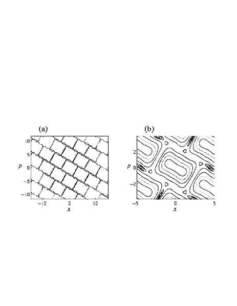
FIG. 2.: Poincaré sections of the phase space dynamics of the classical delta-kicked harmonic oscillator. (a) Single unstable initial condition forming a stochastic web spreading through phase space. (b) Close up of the phase space, showing the closed curves characteristic of regular dynamics. In both cases $\tau_{h}=2\pi/6$, $\kappa=1$.

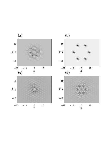
FIG. 3.: Pseudocolour plot of time averaged Wigner functions when $\upsilon=0$, i.e. linear Schrödinger equation dynamics, in the two cases of: $\eta=1$, for (a) unstable initial condition, (b) stable initial condition; $\eta=2$, for (c) unstable initial condition, (d) stable initial condition. Position and momentum are scaled in harmonic units, and black means large and positive.

FIG. 4.: As for Fig. 3, where $\upsilon=0.1$.

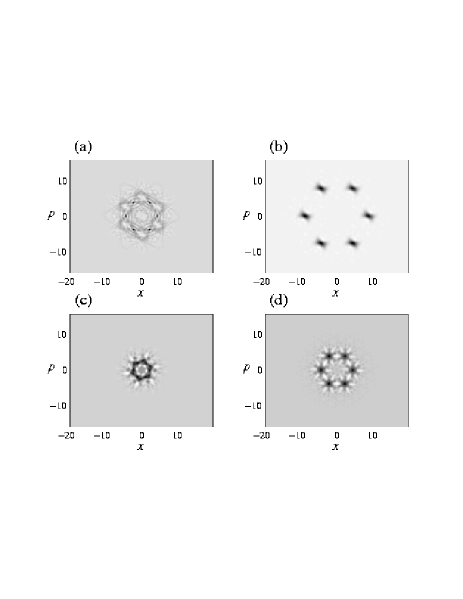
FIG. 5.: As for Fig.3, where $\upsilon=1$.

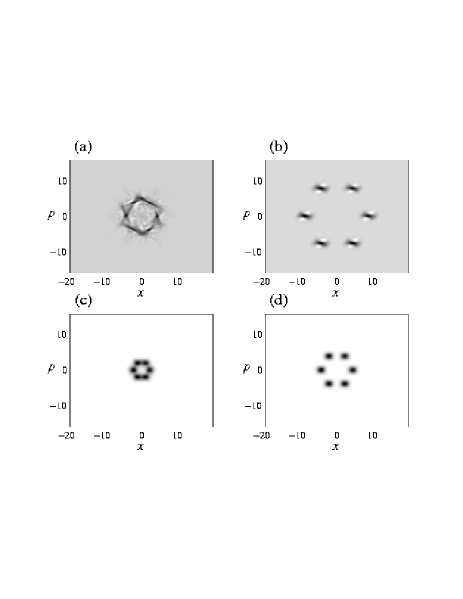
FIG. 6.: As for Fig. 3, where $\upsilon=10$.

FIG. 7.: Pseudocolour plot of time averaged distributions undergoing Liouville dynamics when $\upsilon=0.1$, in the two cases of: $\eta=1$, for (a) unstable initial condition, (b) stable initial condition; $\eta=2$, for (a) unstable initial condition, (b) stable initial condition. Black means large and positive.

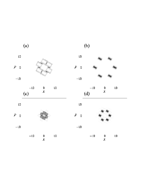
FIG. 8.: As for Fig. 7 when $\upsilon=1$.

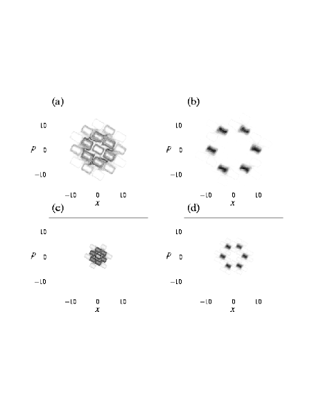
FIG. 9.: As for Fig. 7 when $\upsilon=10$.

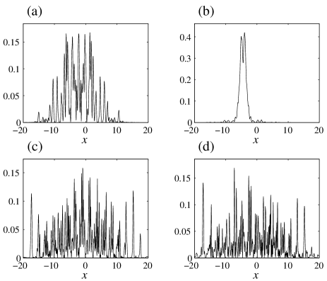
FIG. 10.: Plots of $|\varphi(x)|^{2}$ after the application of 100 kicks and where $\upsilon=0.1$, in the cases of: $\eta=1$, for (a) unstable initial condition, (b) stable initial condition; and $\eta=2$, for (c) unstable initial condition, (d) stable initial condition.

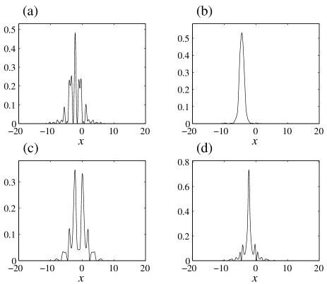
FIG. 11.: As for Fig. 10, but for $\upsilon=1$.

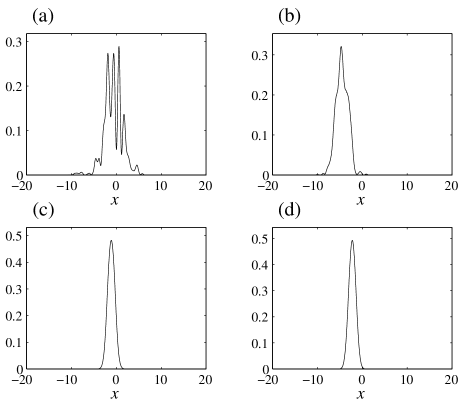
FIG. 12.: As for Fig. 10, but for $\upsilon=10$.

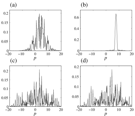
FIG. 13.: Plots of $|\varphi(p)|^{2}$ after the application of 100 kicks and where $\upsilon=0.1$, in the cases of: $\eta=1$, for (a) unstable initial condition, (b) stable initial condition; and $\eta=2$, for (c) unstable initial condition, (d) stable initial condition.

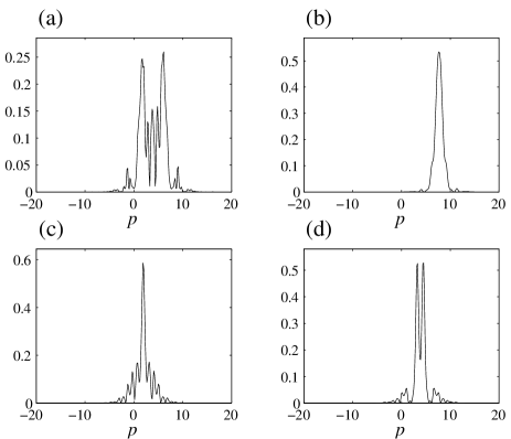
FIG. 14.: As for Fig. 13, but for $\upsilon=1$.

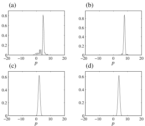
FIG. 15.: As for Fig. 13, but for $\upsilon=10$.

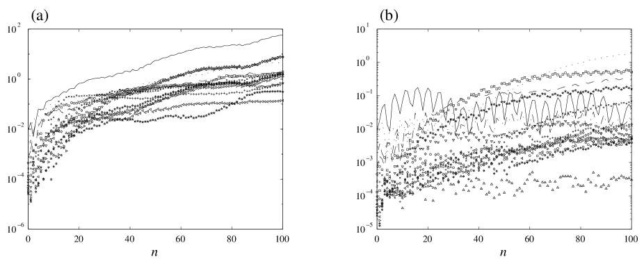
FIG. 16.: Semilog plot of change in $\langle v_{k}|v_{k}\rangle$ with respect to the number of kicks $n$, for $k=1,\ldots,15$: $k=1$ solid line, $k=2$ dotted line, $k=3$ dashed-dotted line, $k=4$ dashed line, $k=5$ circles, $k=6$ crosses, $k=7$ pluses, $k=8$ squares, $k=9$ diamonds, $k=10$ downward pointing triangles, $k=11$ upward pointing triangles, $k=12$ left pointing triangles, $k=13$ right pointing triangles, $k=14$ pentagrams, $k=15$ hexagrams, where $\eta^{\prime}=1$, and $\upsilon=1$. (a) shows data for the “unstable” initial condition, where the leading term after 100 kicks is for $k=1$, (b) shows data for the “stable” initial condition, where the leading term corresponds to $k=2$.

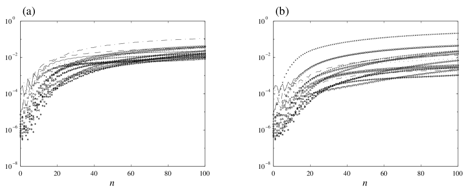
FIG. 17.: As for Fig.16, except that $\eta^{\prime}=2$, $\upsilon=1$. In (a) the leading term is for $k=3$, in (b) for $k=6$.

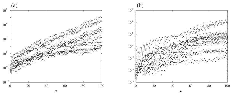
FIG. 18.: As for Fig.16, except that $\eta^{\prime}=1$, $\upsilon=10$. In (a) the leading term is for $k=1$, in (b) for $k=1,5$.

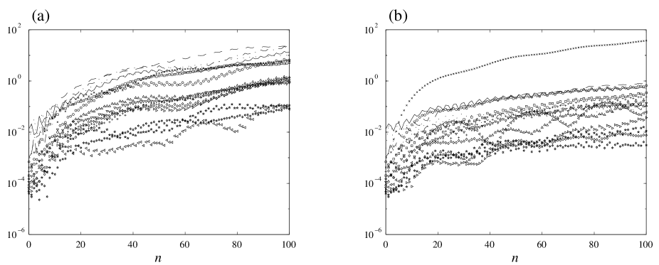
FIG. 19.: As for Fig.16, except that $\eta^{\prime}=2$, $\upsilon=10$. In (a) the leading term is for $k=4$, in (b) for $k=6$.

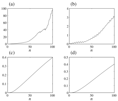
FIG. 20.: Plots of $\sum_{k=1}^{15}\langle v_{k}|v_{k}\rangle$ against the number of kicks $n$, where $\upsilon=1$, in the two cases of: $\eta^{\prime}=1$, for (a) unstable initial condition, (b) stable initial condition; $\eta^{\prime}=2$, (c) unstable initial condition. (d) stable initial condition.

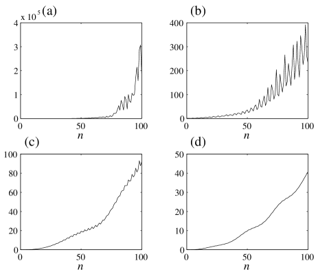
FIG. 21.: Corresponds exactly to Fig. 20, except that $\upsilon=10$.

			Na23		Rb87
$\upsilon$	$\eta^{\prime}$	$\mu$	$\lambda$	$\nu$	$\lambda$	$\nu$
1	1	$0.87\hbar\omega$	$9.55\times 10^{3}s^{-1/2}$	$3.02\times 10^{3}s^{-1/2}$	$2.65\times 10^{3}s^{-1/2}$	$8.38\times 10^{2}s^{-1/2}$
	2	$0.55\hbar\omega$	$1.19\times 10^{3}s^{-1/2}$	$3.77\times 10^{2}s^{-1/2}$	$3.31\times 10^{2}s^{-1/2}$	$1.05\times 10^{2}s^{-1/2}$
10	1	$3.11\hbar\omega$	$9.55\times 10^{4}s^{-1/2}$	$3.02\times 10^{4}s^{-1/2}$	$2.65\times 10^{4}s^{-1/2}$	$8.38\times 10^{3}s^{-1/2}$
	2	$0.95\hbar\omega$	$1.19\times 10^{4}s^{-1/2}$	$3.77\times 10^{3}s^{-1/2}$	$3.31\times 10^{3}s^{-1/2}$	$1.05\times 10^{3}s^{-1/2}$

TABLE I.: Values of $\lambda$ and $\nu$ for Sodium 23 and Rubidium 87, when in the parameter regimes of $\upsilon$ and $\eta^{\prime}$ under study. Also displayed are the values of the numerically determined ground state chemical potential $\mu$ for the appropriate values of $\upsilon$ and $\eta^{\prime}$, in units of $\hbar\omega$.

REFERENCES

- [1] L. E. Reichl The Transition to Chaos In Conservative Classical Systems: Quantum Manifestations (Springer-Verlag, New York 1992).
- [2] M. C. Gutzwiller Chaos in Classical and Quantum Mechanics (Springer-Verlag, Berlin 1990).
- [3] F. Haake, Quantum Signatures of Chaos (Springer-Verlag, Berlin 1991).
- [4] A. Peres, in Quantum Chaos: Proceedings of the Adriatico Research Conference on Quantum Chaos, edited by H. A. Cerdeira, R. Ramaswamy, M. C. Gutzwiller, and G. Casati (World Scientific, Singapore, 1991); A. Peres, Quantum Theory: Concepts and Methods (Kluwer Academic Publishers, Dordrecht 1993); for alternative treatments see also R. Schack and C. M. Caves Phys. Rev. E 53, 3257 (1996); R. Schack and C. M. Caves Phys. Rev. E 53, 3387 (1996); and G. Garcia de Polavieja, Phys. Rev. A 57, 3184 (1998).
- [5] W. H. Zurek and J. P. Paz, Phys. Rev. Lett. 72, 2508 (1994); W. H. Zurek and J. P. Paz, Nuov. Cim. B 110, 611 (1995).
- [6] N. Finlayson, K. J. Blow, L. J. Bernstein, and K. W. Delong, Phys. Rev. A 48, 3863 (1993); F. Benvenuto, G. Casati, A. Pikovsky, and D. L. Shepelyansky, Phys. Rev. A 44, R3423 (1994); B. M. Herbst and M. J. Ablowitz, Phys. Rev. Lett. 18, 2065 (1989).
- [7] G. Baym and C. Pethick, Phys. Rev. Lett. 76, 6 (1996);
- [8] F. Dalfovo, S. Giorgini, L. P. Pitaevskii, and S. Stringari, Rev. Mod. Phys. 71, 463 (1999).
- [9] Y. R. Shen Principles of Nonlinear Optics (Wiley & Sons, New York 1984); R. W. Boyd Nonlinear Optics (Academic Press, San Diego 1992).
- [10] S. Stringari, Phys. Rev. A 58, 2385 (1998); M. Fliesser, A. Csordás, P. Szépfalusy, and R. Graham, Phys. Rev. A 56, R2533 (1997); S. Stringari, Phys. Rev. Lett. 77, 2360 (1996).
- [11] It is more conventional to describe the hydrodynamic equations in terms of a velocity field , as in [8, 10]. We use because in this way it is easier to have a consistent notation for the higher order moments that appear in Sec. III.
- [12] H. Goldstein, Classical Mechanics (Addison-Wesley, Reading 1980).
- [13] Similar hydrodynamic expansions have been carried out for the linear Schrödinger equation, see: J. V. Lill, M. I. Haftel, and G. H. Herling Phys. Rev. A 39, 5832 (1989); J. V. Lill, M. I. Haftel, and G. H. Herling J. Chem. Phys. 90, 4940 (1989); M. Ploszajczak and M. J. Rhoades Brown, Phys. Rev. Lett. 55, 147 (1985); M. Ploszajczak and M. J. Rhoades Brown, Phys. Rev. D 33, 3686 (1986).
- [14] G. M. Zaslavskiĭ, M. Yu. Zakharov, R. Z. Sagdeev, D. A. Usikov, and A. A. Chernikov, JETP Lett. 44, 451 (1986); G. M. Zaslavskiĭ, M. Yu. Zakharov, R. Z. Sagdeev, D. A. Usikov, and A. A. Chernikov, Sov. Phys. JETP 64, 294 (1986); A. A. Chernikov, R. Z. Sagdeev, D. A. Usikov, M. Yu. Zakharov, and G. M. Zaslavsky, Nature 326, 559 (1987).
- [15] A. A. Chernikov, R. Z. Sagdeev, and G. M. Zaslavsky, Physica D 33, 65 (1988).
- [16] V. V. Afanasiev, A. A. Chernikov, R. Z. Sagdeev, and G. M. Zaslavsky, Phys. Lett. A 144, 229 (1990).
- [17] A. A. Chernikov, R. Z. Sagdeev, D. A. Usikov, and G. M. Zaslavsky, Computers Math. Applic. 17, 17 (1989).
- [18] G. P. Berman, V. Yu. Rubaev, and G. M. Zaslavsky, Nonlinearity 4, 543 (1991)
- [19] F. Borgonovi and L. Rebuzzini, Phys. Rev. E 52, 2302 (1995). The possibility of extended eigenstates was also investigated in [18].
- [20] M. Frasca, Phys. Lett. A 231, 344 (1997).
- [21] T. Hogg and B. A. Huberman, Phys. Rev. A 28, 28 (1983).
- [22] V. I. Arnol’d, Sov. Math. Doklady 5, 581 (1964), reprinted in Hamiltonian Dynamical Systems, edited by R. S. MacKay and J. D. Meiss (Adam Kilger, Bristol 1986).
- [23] A. N. Kolmogorov, Dokl. Akad. Nauk. SSSR 98, 527 (1954); V. I. Arnol’d, Russ. Math. Survey 18, 9, 85 (1963); J. Moser, Nachr. Akad. Wiss. Göttingen II, Math. Phys. Kl. 18, 1 (1962).
- [24] W. Kohn, Phys. Rev. 4, 1242 (1961); S. A. Morgan, R. J. Ballagh, and K. Burnett, Phys. Rev. A 55, 4338 (1997).
- [25] F. L. Moore, J. C. Robinson, C. Bharucha, P. E. Williams, and M. G. Raizen, Phys. Rev. Lett. 73, 2974 (1994); J. C. Robinson, C. Bharucha, F. L. Moore, R. Jahnke, G. A. Georgakis, Q. Niu, M. G. Raizen, and B. Sundaram, Phys. Rev. Lett. 74, 3963 (1995); J. C. Robinson, C. F. Bharucha, K. W. Madison, F. L. Moore, Bala Sundaram, S. R. Wilkinson, and M. G. Raizen, Phys. Rev. Lett. 76, 3304 (1996); B. G. Klappauf, W. H. Oskay, D. A. Steck, and M. G. Raizen Phys. Rev. Lett. 81, 1203 (1998); B. G. Klappauf, W. H. Oskay, D. A. Steck, and M. G. Raizen Phys. Rev. Lett. 81, 4044 (1998). In the context of quantum chaos significant experimental work has been carried out on microwave driven hydrogen [39] and mesoscopic solid state systems [40].
- [26] S. A. Gardiner, J. I. Cirac, and P. Zoller, Phys. Rev. Lett. 79, 4790 (1997).
- [27] We use the formalism of Y. Castin and R. Dum, Phys. Rev. A 57, 3008 (1998), an analogous formalism is presented in C. W. Gardiner, Phys. Rev. A 56, 1414 (1997); see also [28].
- [28] Y. Castin and R. Dum, Phys. Rev. Lett. 79, 3553 (1997).
- [29] C. C. Marston and G. G. Balint-Kurti, J. Chem. Phys. 91, 3571 (1989).
- [30] J. L. Roberts, N. R. Claussen, J. P. Burke, Jr., C. H. Greene, E. A. Cornell, and C. E. Wieman, Phys. Rev. Lett. 81, 5109 (1998).
- [31] J. Stenger, S. Inouye, M. R. Andrews, H.-J. Miesner, D. M. Stamper-Kurn, and W. Ketterle, Phys. Rev. Lett. 82, 2422 (1999).
- [32] J. E. Moyal, Proc. Cambridge Phil. Soc. 45, 99 (1949).
- [33] E. P. Wigner, Phys. Rev. 40, 749 (1932).
- [34] L. Fejes Tóth Regular Figures (Pergamon, Oxford 1964).
- [35] C. W. Curtis and I. Reiner Theory of Finite Groups and Associative Algebras (Wiley-Interscience, New York 1962).
- [36] D. F. Walls and G. J. Milburn Quantum Optics (Springer-Verlag, Berlin 1994).
- [37] F. M. Izrailev and D. L. Shepelyanskii, Sov. Phys. Dokl. 24, 996 (1980); F. M. Izrailev and D. L. Shepelyanskii, Theor. Math. Phys. 43, 553 (1980); D. R. Grempel, S. Fishman, and R. E. Prange, Phys. Rev. Lett. 49, 833 (1982); D. R. Grempel, R. E. Prange, and S. Fishman, Phys. Rev. A 29, 1639 (1984).
- [38] See, for example A. D. Bandrauk and H. Shen, J. Phys. A 27, 7147 (1994), and references therein.
- [39] E. Doron, U. Smilansky, and A. Frenkel, Phys. Rev. Lett. 65, 3072 (1990); J. E. Bayfield, G. Casati, I. Guarneri, and D. W. Sokol, Phys. Rev. Lett. 63, 364 (1989); E. J. Galvez, B. E. Sauer, L. Moorman, P. M. Koch, and M. Richards, Phys. Rev. Lett. 61, 2011 (1988); for a review see P. M. Koch and K. A. H. van Leeuwen, Phys. Rep. 255, 289 (1995).
- [40] P. B. Wilkinson, T. M. Fromhold, L. Eaves, F. W. Sheard, N. Miura, and T. Takamasu, Nature 380, 608 (1996); T. M. Fromhold, P. B. Wilkinson, F. W. Sheard, L. Eaves, J. Miao, and G. Edwards, Phys. Rev. Lett. 75, 1142 (1995).