Evaluating Capacities of Bosonic Gaussian Channels

Abstract

We show how to compute or at least to estimate various capacity-related quantities for Bosonic Gaussian channels. Among these are the coherent information, the entanglement assisted classical capacity, the one-shot classical capacity, and a new quantity involving the transpose operation, shown to be a general upper bound on the quantum capacity, even allowing for finite errors. All bounds are explicitly evaluated for the case of a one-mode channel with attenuation/amplification and classical noise.

I Introduction

During the last years impressive progress was achieved in the understanding of the classical and quantum capacities of quantum communication channels (see, in particular, the papers [1] - [6], where the reader can also find further references). It appears that a quantum channel is characterized by a whole variety of different capacities depending both on the kind of the information transmitted and the specific protocol used.

Most of this literature studies the properties of systems and channels described in finite dimensional Hilbert spaces. Recently, however, there has been a burst of interest (see e. g. [7]) in a new kind of systems, sometimes called “continuous variable” quantum systems, whose basic variables satisfy Heisenberg’s Canonical Commutation Relations (CCR). There are two reasons for this new interest. On the one hand, such systems play a central role in quantum optics, the canonical variables being the quadratures of the field. Therefore some of the current experimental realizations [8] of quantum information processing are carried out in such systems. In particular, the Bosonic Gaussian channels studied in this paper can be seen as basic building blocks of quantum optical communication systems, allowing to build up complex operations from “easy, linear” ones and a few basic “expensive, non-linear” operations, such as squeezers and parametric down converters.

The other reason for the interest in these systems is that in spite of the infinite dimension of their underlying Hilbert spaces they can be handled with techniques from finite dimensional linear algebra, much in analogy to the finite dimensional quantum systems on which the pioneering work on quantum information was done. Roughly speaking this analogy replaces the density matrix by the covariance matrix of a Gaussian state. Then operations like the diagonalization of density matrices, the Schmidt decomposition of pure states on composite systems, the purification of mixed states, the computation of entropies, the partial transpose operation on states and channels, which are familiar from the usual finite dimensional setup, can be expressed once again by operations on finite dimensional matrices in the continuous variable case. The basic framework for doing all this is not new, and goes under heading “phase space quantum mechanics” or, in the quantum field theory and statistical mechanics communities, “quasi-free Bose systems” [9]. Both authors of this paper have participated in the development of this subject a long time ago [10, 11, 12]. In this paper, continuing [13] and [14], we make further contributions to the study of information properties of linear Bosonic Gaussian channels. We focus on the aspects essential for physical computations and leave aside a number of analytical subtleties related to infinite dimensionality and unboundedness unavoidably arising in connection with Bosonic systems and Gaussian states.

The paper is organized as follows. In the Section II we recapitulate some notions of capacity, which are currently under investigation in the literature, and what is known about them. Naturally this cannot be a full review, but will be limited to those quantities which we will evaluate or estimate in the subsequent sections. A new addition to the spectrum of capacity-like quantities is discussed in Subsection II.B: an upper bound on the quantum capacity (even allowing finite errors), which is both simple to evaluate and remarkably close to maximized coherent information, a bound conjectured to be exact. In Section III we summarize the basic properties of Gaussian states. Although our main topic is channels, we need this to get an explicit handle on the purification operation, which is needed to compute the entropy exchange, and hence all entropy based capacities. Bosonic Gaussian channels are studied in Section IV. Here we introduce the techniques for determining the capacity quantities introduced in Section I, deriving general formulas where possible. In the final Section V we apply these techniques to the case of a single mode channel comprising attenuation/amplification and a classical noise. Some technical points are treated in the Appendices.

II Notions of capacity

A Basic entropy and information quantities

Consider a general quantum system in a Hilbert space ${\cal H=H}_{Q}$. Its states are given by density operators $\rho$ on ${\cal H}$. A channel is a transformation $\rho\rightarrow T[\rho]$ of quantum states of the system, which is given by a completely positive, trace preserving map on trace class operators. This view of channels corresponds to the Schrödinger picture. The Heisenberg picture is given by the dual linear operator $X\rightarrow T^{*}[X]$ on the observables $X$, which is defined by the relation

$\displaystyle{\rm Tr}T[\rho]X={\rm Tr}\rho T^{*}[X],$

and has to be completely positive and unit preserving (cf. [15]).

It can be shown (see e.g. [16]) that any channel in this sense arises from a unitary interaction $U$ of the system with an environment described by another Hilbert space ${\cal H}_{E}$ which is initially in some state $\rho_{E}$,

$\displaystyle T[\rho]={\rm Tr}_{E}U\left(\rho\otimes\rho_{E}\right)U^{*},$

where ${\rm Tr}_{E}$ denotes partial trace with respect to ${\cal H}_{E}$, and vice versa. The representation is not unique, and the state $\rho_{E}$ can always be chosen pure, $\rho_{E}=|\psi_{E}\rangle\langle\psi_{E}|$. The definition of the channel has obvious generalization to the case where input and output are described by different Hilbert spaces.

Let us denote by

$$H(\rho)=-{\rm Tr}\rho\log\,\rho$$ (2.1)

the von Neumann entropy of a density operator $\rho$. We call $\rho$ the input state, and $T[\rho]$ the output state of the channel. There are three important entropy quantities related to the pair $(\rho,T)$, namely, the entropy of the input state $H(\rho)$, the entropy of the output state $H(T[\rho])$, and the entropy exchange $H(\rho,T)$. While the definition and the meaning of the first two entropies is clear, the third quantity is somewhat more sophisticated. To define it, one introduces the reference system, described by the Hilbert space ${\cal H}_{R}$, isomorphic to the Hilbert space ${\cal H}_{Q}=$ ${\cal H}$ of the initial system. Then according to [17], [3], there exists a purification of the state $\rho$, i.e. a unit vector $|\psi\rangle\in{\cal H}_{Q}\otimes{\cal H}_{R}$ such that

$\displaystyle\rho={\rm Tr}_{R}|\psi\rangle\langle\psi|.$

The entropy exchange is then defined as

$$H(\rho,T)=H\bigl{(}(T\otimes{\rm id})[|\psi\rangle\langle\psi|]\bigr{)},$$ (2.2)

that is, as the entropy of the output state of the dilated channel $(T\otimes{\rm id})$ applied to the input which is purification of the state $\rho$. Alternatively,

$\displaystyle H(\rho,T)=H(\rho_{E}^{\prime}),$

where $\rho_{E}^{\prime}=T_{E}[\rho]$ is the final state of the environment, and the channel $T_{E}$ from ${\cal H}_{Q}$ to ${\cal H}_{E}$ is defined as

$\displaystyle T_{E}[\rho]={\rm Tr}_{Q}U\left(\rho\otimes\rho_{E}\right)U^{*},$

provided the initial state $\rho_{E}$ of the environment is pure [17], [3].

¿From these three entropies one can construct several information quantities. In analogy with classical information theory, one can define quantum mutual information between the reference system $R$ (which mirrors the input $Q$) and the output of the system $Q^{\prime}$ [17], [4] as

$$I(\rho,T) = H(\rho_{R}^{\prime})+H(\rho_{Q}^{\prime})-H(\rho_{RQ}^{\prime})$$ (2.3)

$$= H(\rho)+H(T[\rho])-H(\rho,T).$$ (2.4)

The quantity $I(\rho,T)$ has a number of nice and “natural” properties, in particular, positivity, concavity with respect to the input state $\rho$ and additivity for parallel channels [4]. Moreover, the maximum of $I(\rho,T)$ with respect to $\rho$ was argued recently to be equal to the entanglement-assisted classical capacity of the channel [6],[18], namely, the classical capacity of the superdense coding protocol using the noisy channel $T$. It was shown that this maximum is additive for parallel channels, the one-shot expression thus giving the full (asymptotic) capacity.

It would be natural to compare this quantity with the (unassisted) classical capacity $C(T)$ (the definition of which is outlined in the next Subsection); however it is still not known whether this capacity is additive for parallel channels. This makes us focus on the one-shot expression, emerging from the coding theorem for classical-quantum channels [2]

$$C_{1}(T)=\max\left[H\Bigl{(}\sum_{i}p_{i}T\left[\rho_{i}\right]\Bigr{)}\right.\left.-\sum_{i}p_{i}H\left(T\left[\rho_{i}\right]\right)\right],$$ (2.5)

where the maximum is taken over all probability distributions $\left\{p_{i}\right\}$ and collections of density operators $\left\{\rho_{i}\right\}$ (possibly satisfying some additional input constraints). $C_{1}(T)$ is equal to the capacity of $T$ for classical information, if the coding is required to avoid entanglement between successive inputs to the channel. The full capacity is then attained as the length $n$ of the blocks, over which encoding may be entangled goes to infinity, i.e.,

$$C(T)=\lim_{n\to\infty}\ \frac{1}{n}C_{1}(T^{\otimes n}).$$ (2.6)

An important component of $I(\rho,T)$ is the coherent information

$$J(\rho,T)=H(T[\rho])-H(\rho,T),$$ (2.7)

the maximum of which has been conjectured to be the (one-shot) quantum capacity of the channel $T$ [19], [3]. Its properties are not so nice. It can be negative, its convexity properties with respect to $\rho$ are not known, and its maximum was shown to be strictly superadditive for certain parallel channels [20], hence the conjectured full quantum capacity may be greater than the one-shot expression, in contrast to the case of the entanglement-assisted classical capacity. In this paper we shall also compare this expression with a new upper bound on the quantum capacity $Q(T)$ (as introduced e.g. in the next Subsection).

B A general bound on quantum channel capacity

In this Subsection we will establish a general estimate on the quantum channel capacity, which will then be evaluated in the Gaussian case, and will be compared with the estimates of coherent information. Let us recall first a definition of the capacity $Q(T)$ of a general channel $T$ for quantum information. Intuitively, it is the number of qubits which can be faithfully transmitted per use of the channel with the best possible error correction. The standard of comparison is the ideal 1-qubit channel ${\rm id}_{2}$, where ${\rm id}_{n}$ denotes the identity map on the $n\times n$-matrices. Then the quantum capacity $Q(T)$ of a channel $T$ (possibly between systems of different type) is defined as the supremum of all numbers $c$, which are “attainable rates” in the following sense: For any pair of sequences $n_{\alpha},m_{\alpha}$ with $\lim_{\alpha}(n_{\alpha}/m_{\alpha})=c$ we can find encoding operations $E_{\alpha}$ and decoding operations $D_{\alpha}$ such that

$\displaystyle\|{\rm id}_{2}^{\otimes n_{\alpha}}-D_{\alpha}T^{\otimes m_{\alpha}}E_{\alpha}\|_{{\rm cb}}\longrightarrow 0.$

Here $\|\cdot\|_{{\rm cb}}$ is the so-called “norm of complete boundedness”[21], which is defined as the supremum with respect to $n$ of the norms $\|(T\otimes{\rm id}_{n})\|$. It is equal to the “diamond metric” introduced in [22]. We use this norm because on the one hand, it leads to the same capacity as analogous definitions based on other error criteria (e.g., fidelities [3, 5]) and, on the other hand, it has the best properties with respect to tensor products, which are our main concern. In particular, $\|T\otimes S\|_{{\rm cb}}=\|T\|_{{\rm cb}}\cdot\|S\|_{{\rm cb}}$. Completely positive maps satisfy $\|T\|_{{\rm cb}}=\|F\|$, where $F$ is the normalization operator determined by ${\rm Tr}(T[\rho])={\rm Tr}(\rho F)$. In particular, $\|T\|_{{\rm cb}}=1$ for any channel. We also note another kind of capacity, in which a much weaker requirement is made on the errors, namely

$$\|{\rm id}_{2}^{\otimes n_{\alpha}}-D_{\alpha}T^{\otimes m_{\alpha}}E_{\alpha}\|_{{\rm cb}}\leq\varepsilon<1$$ (2.8)

for all sufficiently large $\alpha$, and some fixed $\varepsilon$. We call the resulting capacity the $\varepsilon$-quantum capacity, and denote it by $Q_{\varepsilon}(T)$. Of course, $Q(T)\leq Q_{\varepsilon}(T)$, and by analogy with the classical case (strong converse of Shannon’s Coding Theorem) one would conjecture that equality always holds.

The unassisted classical capacity $C(T)$ can be defined similarly with the sole difference that both the domain of encodings $E$ and the range of decodings $D$ should be restricted to the state space of the Abelian subalgebra of operators diagonalizable in a fixed orthonormal basis. In that case there is no need to use the cb-norm, as it coincides with the usual norm. According to recently proven strong converse to the quantum coding theorem [23], [24], $C_{\varepsilon}(T)=C(T)$ where $C_{\varepsilon}(T)$ is defined similarly to $Q_{\varepsilon}(T)$.

The criterion we will formulate makes essential use of the transpose operation, which we will denote by the same letter $\Theta$ in any system. For matrix algebras, $\Theta$ can be taken as the usual transpose operation. However, it makes no difference to our considerations, if any other anti-unitarily implemented symmetry (e.g. time-reversal) is chosen. In an abstract C*-algebra setting $\Theta$ is best taken as the “op” operation, which maps every algebra to its “opposite”. This algebra has the same underlying vector space, but all products $AB$ are replaced by their opposite $BA$. Obviously, a commutative algebra is the same as its opposite, so on classical systems $\Theta$ is the identity. Although the transpose maps density operators to density operators, it is not an admissible quantum channel, because positivity is lost, when coupling the operation with the identity transformation on other systems, i.e., $\Theta$ is not completely positive. A similar phenomenon happens for the norm of $\Theta$: we have $\|\Theta\|_{{\rm cb}}>1$ unless the system is classical. In fact,

$$\|\Theta_{n}\|_{{\rm cb}}=n,$$ (2.9)

where $\Theta_{n}$ denotes the transposition on the $n\times n$-matrices [21]. We note that since we do not distinguish the transpose on different systems in our notation, the observation that tensor products can be transposed factor by factor is expressed by the equation $\Theta=\Theta\otimes\Theta$. Moreover, although for a channel $T$, the operator $T\Theta$ may fail to be completely positive, $\Theta T\Theta$ is again a channel, and, in particular, satisfies $\|\Theta T\Theta\|_{{\rm cb}}=1$.

The main result of this Subsection is the estimate

$$Q_{\varepsilon}(T)\leq\log\|T\Theta\|_{{\rm cb}}\equiv Q_{\Theta}(T),$$ (2.10)

for any channel $T$. The proof is quite simple. Suppose $n_{\alpha}/m_{\alpha}\rightarrow c\leq Q_{\varepsilon}(T)$, and encoding $E_{\alpha}$ and decoding $D_{\alpha}$ are as in the definition of $Q_{\varepsilon}(T)$. Then by Equation ( 2.9) we have

$$2^{n_{\alpha}} = \|{\rm id}_{2}^{\otimes n_{\alpha}}\Theta\|_{{\rm cb}}\ \leq$$ (2.11)

$$\leq \|({\rm id}_{2}^{\otimes n_{\alpha}}-D_{\alpha}T^{\otimes m_{\alpha}}E_{\alpha})\Theta\|_{{\rm cb}}$$ (2.13)

$$\qquad+\|D_{\alpha}T^{\otimes m_{\alpha}}E_{\alpha}\Theta\|_{{\rm cb}}$$

$$\leq \|\Theta_{2^{n_{\alpha}}}\|_{{\rm cb}}\ \|{\rm id}_{2}^{\otimes n_{\alpha}}-D_{\alpha}T^{\otimes m_{\alpha}}E_{\alpha}\|_{{\rm cb}}$$ (2.15)

$$\qquad+\|D_{\alpha}(T\Theta)^{\otimes m_{\alpha}}\Theta E_{\alpha}\Theta\|_{{\rm cb}}$$

$$\leq 2^{n_{\alpha}}\varepsilon+\|T\Theta\|_{{\rm cb}}^{m_{\alpha}},$$ (2.16)

where at the last inequality we have used that $D_{\alpha}$ and $\Theta E_{\alpha}\Theta$ are channels, and that the cb-norm is exactly tensor multiplicative, so $\|X^{\otimes m}\|_{{\rm cb}}=\|X\|_{{\rm cb}}^{m}$. Hence, by taking the logarithm and dividing by $m_{\alpha}$, we get

$\displaystyle\frac{n_{\alpha}}{m_{\alpha}}\log 2+\frac{\log(1-\varepsilon)}{m_{\alpha}}\leq\log\|T\Theta\|_{{\rm cb}}.$

If we take base $2$ logarithms, as is customary in information theory, we have $\log 2=1$. Then in the last inequality we can go to the limit $\alpha\to\infty$, obtaining $c\leq Q_{\Theta}(T)$, and Equation (2.10) follows by taking the supremum over all attainable rates $c$. Note that base $2$ logarithms are built into the above definition of capacity, because we are using the ideal qubit channel as the standard of comparison. This amounts only to a change of units. If another base is chosen for logarithms is chosen, this should also be done consistently in all entropy expressions, and Equation (2.10) holds once again without additional constants.

The upper bound $Q_{\Theta}(T)$ computed in this way has some remarkable properties, which make it a capacity-like quantity in its own right. For example, it is exactly additive:

$$Q_{\Theta}(S\otimes T)=Q_{\Theta}(S)+Q_{\Theta}(T),$$ (2.17)

for any pair $S,T$ of channels, and satisfies the “bottleneck inequality” $Q_{\Theta}(ST)\leq\min\{Q_{\Theta}(S),Q_{\Theta}(T)\}$. Moreover, it coincides with the quantum capacity on ideal channels: $Q_{\Theta}({\rm id}_{n})=Q({\rm id}_{n})=\log_{2}n$, and it vanishes whenever $T\Theta$ is completely positive. In particular, $Q_{\Theta}(T)=0$, whenever $T$ is separable in the sense that it can be decomposed as $T=PM$ into a measurement $M$ and a subsequent preparation $P$ based on the measurement results. This follows immediately from the observation that on classical systems transposition is the identity. Then $P\Theta=\Theta P\Theta$ is a channel, and so is $MP\Theta$. We note that $Q_{\Theta}$ is also closely related to the entanglement quantity $\log_{2}\|({\rm id}\otimes\Theta)(\rho)\|_{1}$, i.e., the logarithm of the trace norm of the partial transpose of the density operator, which enjoys analogous properties.

III Quantum Gaussian states

A Canonical Variables and Gaussian states

In this Section we recapitulate some results from [10], [13], [14] for the convenience of the reader. Our approach to quantum Gaussian states is based on the characteristic function of the state which closely parallels classical probability [11], [12], and is perhaps the simplest and most transparent analytically. An alternative approach can be based on the Wigner “distribution function” [25].

Let $q_{j},p_{j}$ be the canonical observables satisfying the Heisenberg CCR

$\displaystyle[q_{j},p_{k}]=i\delta_{jk}\hbar I,\;\;[q_{j},q_{k}]=0,\;\;[p_{j},p_{k}]=0.$

We introduce the column vector of operators

$\displaystyle R=[q_{1},p_{1},\dots,q_{s},p_{s}]^{T},$

the real column $2s$-vector $z=[x_{1},y_{1},\dots,x_{s},y_{s}]^{T}$, and the unitary operators in ${\cal H}$

$$V(z) = \exp\,i\sum_{j=1}^{s}(x_{j}q_{j}+y_{j}p_{j})$$ (3.18)

$$= \exp\,i\,R^{T}z.$$ (3.19)

These “Weyl-operators” satisfy the Weyl-Segal CCR

$$V(z)V(z^{\prime})=\exp[\frac{i}{2}\Delta(z,z^{\prime})]V(z+z^{\prime}),$$ (3.20)

where

$$\Delta(z,z^{\prime})=\hbar\sum_{j=1}^{s}(x_{j}^{\prime}y_{j}-x_{j}y_{j}^{\prime})$$ (3.21)

is the canonical symplectic form. The space $Z$ of real $2s$-vectors equipped with the form $\Delta(z,z^{\prime})$ is what one calls a symplectic vector space. We denote by

$$\Delta=\left[\begin{array}[]{ccccc}0&\hbar&&&\\ -\hbar&0&&&\\ &&\ddots&&\\ &&&0&\hbar\\ &&&-\hbar&0\end{array}\right]$$ (3.22)

the $(2s)\times(2s)$-skew-symmetric commutation matrix of components of the vector $R$, so that

$\displaystyle\Delta(z,z^{\prime})=-z^{T}\Delta z^{\prime}.$

Most of the results below are valid for the case where the commutation matrix is an arbitrary (nondegenerate) skew-symmetric matrix, not necessarily of the canonical form (3.22).

A density operator $\rho$ has finite second moments if ${\rm Tr}(\rho q_{j}^{2})<\infty$ and ${\rm Tr}(\rho p_{j}^{2})<\infty$ for all $j$. In this case one can define the vector mean and the correlation matrix $\alpha$ by the formulas

$$m={\rm Tr}\rho R\;;\;\alpha-\frac{i}{2}\Delta={\rm Tr}(R-m)\rho(R-m)^{T}.$$ (3.23)

The mean can be an arbitrary real vector. The correlation matrix $\alpha$ is real and symmetric. A given $\alpha$ is the correlation matrix of some state if and only if it satisfies the matrix uncertainty relation

$$\alpha-\frac{i}{2}\Delta\geq 0.$$ (3.24)

We denote by $\Sigma\left(m,\alpha\right)$ the set of states with fixed mean $m$ and the correlation function $\alpha$. The density operator $\rho$ is called Gaussian, if its quantum characteristic function $\phi(z)={\rm Tr}\rho V(z)$ has the form

$$\phi(z)=\exp\left(i\,m^{T}z-\frac{1}{2}z^{T}\alpha z\right),$$ (3.25)

where $m$ is a column ($2s$)-vector and $\alpha$ is a real symmetric $(2s)\times(2s)$-matrix. One then can show that $m$ is indeed the mean, and $\alpha$ is the correlation matrix, and (3.25) defines the unique Gaussian state in $\Sigma\left(m,\alpha\right)$. In what follows we will be interested mainly in the case $m=0$.

The correlation matrix $\alpha$ describes a quadratic form rather than an operator. Therefore its eigenvalues have no intrinsic significance, and depend on the choice of basis in $Z$. On the other hand, the operator $\widehat{\alpha}$ defined by $z^{T}\alpha z=\Delta(z,\widehat{\alpha}z)$ has a basis free meaning. In matrix notation it is $\widehat{\alpha}=\Delta^{-1}\alpha$. This operator is always diagonalizable, and its eigenvalues come in pairs $\pm i\gamma_{j}$. Diagonalizing this operator is essentially the same as the normal mode decomposition of the phase space, when the form $z^{T}\alpha z$ is considered as the Hamiltonian function of a system of oscillators. It leads to a decomposition of the phase space into two-dimensional subspaces, such that on the $j^{\rm th}$ subspace we have (in some new canonical variables ${\tilde{q}}_{j},{\tilde{p}}_{j}$)

$$\alpha=\hbar\left[\begin{array}[]{ll}\gamma_{j}&0\\ 0&\gamma_{j}\end{array}\right]\quad;\quad\Delta=\hbar\left[\begin{array}[]{ll}0&1\\ -1&0\end{array}\right],$$ (3.26)

and all terms between different blocks vanish. The matrix uncertainty relation now requires $\gamma_{j}\geq 1/2$, in which equality holds iff $\rho_{j}$ is the pure (minimum-uncertainty) state. Hence a general Gaussian state $\rho$ is pure if and only if all $\gamma_{j}=1/2$, or

$$(\Delta^{-1}\alpha)^{2}=-\ \frac{1}{4}I,$$ (3.27)

in which case $\Sigma\left(m,\alpha\right)$ reduces to a single point.

B Gauge-invariant states

We shall be interested in the particular subclass of Gaussian states most familiar in quantum optics, namely, the states having a P-representation

$$\rho=\int|\zeta\rangle\langle\zeta|\mu_{N}(d^{2s}\zeta)$$ (3.28)

where $\mu_{N}(d^{2s}\zeta)$ is the complex Gaussian probability measure with zero mean and the correlation matrix $N$. (see e.g. [26], Sec. V, 5. II). Here $\zeta\in{\bf C}^{s}$, $|\zeta\rangle$ are the coherent vectors in ${\cal H}$, $a|\zeta\rangle=\zeta|\zeta\rangle$, $N$ is positive Hermitian matrix such that

$$N={\rm Tr}\left(a\,\rho\,a^{\dagger}\right)$$ (3.29)

(we use here vector notations, where $a=[a_{1},\dots,a_{s}]^{T}$ is a column vector and $a^{\dagger}=[a_{1}^{\dagger},\dots,a_{s}^{\dagger}]$ is a row vector) and $a_{j}=\frac{1}{\sqrt{2\hbar}}(q_{j}+ip_{j})$.

These states respect the natural complex structure in the sense that they are invariant under the gauge transformations $a\rightarrow a\exp(i\varphi)$. As shown in [13], the quantum correlation matrix of such states is

$\displaystyle\alpha=\hbar\left[\begin{array}[]{ll}{\rm Re}N+I/2&-{\rm Im}N\\ {\rm Im}N&{\rm Re}N+I/2\end{array}\right],$

With Pauli matrices $I_{2},\sigma_{y}$, the real $2s\times 2s-$ matrices of such form can be rewritten as complex $s\times s-$ matrices, by using the correspondence

$\displaystyle\left[\begin{array}[]{ll}A&-B\\ B&A\end{array}\right]=I_{2}A+\sigma_{y}B\leftrightarrow A+iB,$

which is an algebraic isomorphism. Obviously,

$\displaystyle\frac{1}{2}{\rm Sp}\left[\begin{array}[]{ll}A&-B\\ B&A\end{array}\right]={\rm Sp}(A+iB),$

where by “${\rm Sp}$” we denote the trace of matrices, as opposed to the trace of Hilbert space operators, which is denoted by “Tr”. By using this correspondence, we have

$$\alpha\leftrightarrow\hbar(N+I/2),\qquad\Delta\leftrightarrow-i\hbar I,$$ (3.30)

and

$$\Delta^{-1}\alpha\leftrightarrow i(N+I/2).$$ (3.31)

For the case of one degree of freedom we shall be interested in the last Section, $N$ is just a nonnegative number and $\rho$ is an elementary Gaussian state with the characteristic function

$$\phi(z)=\exp\left[-\frac{\hbar}{2}\left(N+\frac{1}{2}\right)|z|^{2}\right],$$ (3.32)

where we put $|z|^{2}=(x^{2}+y^{2})$. This state has correlation matrix of the form (3.26) in the initial variables $q,p$, with $\gamma=N+1/2$, and is just the temperature state of the harmonic oscillator

$$\rho_{\gamma}=\frac{1}{\gamma+1/2}\sum_{n=0}^{\infty}\left(\frac{\gamma-1/2}{\gamma+1/2}\right)^{n}\ |n\rangle\,\langle n|$$ (3.33)

in the number basis $|n\rangle$, with the mean photon number $N$.

C Computation of entropy

To compute the von Neumann entropy of a general Gaussian state one can use the normal mode decomposition. For a single mode, the density operator $\rho_{j}$ with the correlation matrix (3.26), setting $\gamma_{j}\equiv\gamma$ for convenience, is unitarily equivalent to the state (3.33). From this one readily gets the von Neumann entropy $H(\rho_{\gamma})$ by summation of the geometric series, and for general Gaussian $\rho$ by summing over normal modes.

To write the result in compact form, one introduces the function

$$g(x) = (x+1)\log(x+1)-x\log x,\quad x>0$$ (3.34)

$$g(0) = 0.$$ (3.35)

Then

$$H(\rho)=\sum_{j=1}^{s}\ g\left(|\gamma_{j}|-\frac{1}{2}\right),$$ (3.36)

where $\gamma_{j}$ runs over all eigenvalue pairs $\pm i\gamma_{j}$ of $\Delta^{-1}\alpha$.

One can also write this more compactly, using the following notations, which we will also use in the sequel. For any diagonalizable matrix $M=S{\rm diag}(m_{j})S^{-1}$, we put ${\rm abs}(M)=S{\rm diag}(|m_{j}|)S^{-1}$, analogously for other continuous functions on the complex plane. Then equation (3.36) can be written as [13]

$$H(\rho)=\frac{1}{2}{\rm Sp}\ g\left({\rm abs}(\Delta^{-1}\alpha)-\frac{I}{2}\right).$$ (3.37)

For gauge-invariant state, by using (3.31), this reduces to the well-known formula

$\displaystyle H(\rho)={\rm Sp}\ g(N).$

D Schmidt Decomposition and Purification

Forming a composite systems out of two systems described by CCR-relations is very simple: one just joins the two sets of canonical operators, making operators belonging to different systems commute. The symplectic space of the composite system is a direct sum $Z_{12}=Z_{1}\oplus Z_{2}$, which means that elements of this space are pairs $(z_{1},z_{2})$ with components $z_{i}\in Z_{i}$. In terms of Weyl operators one can write $V_{12}(z_{1},z_{2})=V_{1}(z_{1})\otimes V_{2}(z_{2})$. By definition, the symplectic matrix $\Delta_{12}$ is block diagonal with respect to the decomposition $Z=Z_{1}\oplus Z_{2}$. However, the correlation matrix $\alpha_{12}$ is block diagonal if and only if the state is a product. The restriction of a bipartite Gaussian state $\rho$ to the first factor is determined by the expectations of the Weyl operators $V_{1}(z_{1})\otimes{\bf 1}=V_{12}(z_{1},0)$, hence according to (3.25), by the the correlation matrix $\alpha_{1}$ with $z_{1}^{T}\alpha_{1}z_{1}=(z_{1},0)^{T}\alpha_{12}(z_{1},0)$, which is just the first diagonal block in the block matrix decomposition

$$\alpha_{12}=\left[\begin{array}[]{ll}\alpha_{1}&\beta\\ \beta^{T}&\alpha_{2}\end{array}\right]\quad;\quad\Delta_{12}=\left[\begin{array}[]{ll}\Delta_{1}&0\\ 0&\Delta_{2}\end{array}\right].$$ (3.38)

As in the case of bipartite systems with finite dimensional Hilbert spaces there is a canonical form for pure states of the composite system, the Schmidt decomposition. Like the diagonalization of a one-site density operator, it can be carried out for Gaussian states at the level of correlation matrices. By writing out equation (3.27) in block matrix form, we find in particular that

$$(\Delta_{1}^{-1}\alpha_{1})(\Delta_{1}^{-1}\beta)=(\Delta_{1}^{-1}\beta)(\Delta_{2}^{-1}\alpha_{2}).$$ (3.39)

Thus $(\Delta_{1}^{-1}\beta)$ maps eigenvectors of $(\Delta_{2}^{-1}\alpha_{2})$ into eigenvectors of $(\Delta_{1}^{-1}\alpha_{1})$, with the same eigenvalue. Hence the spectra of the restrictions are synchronized much in the same way as in the finite dimensional case, and all the matrices $\alpha_{1},\alpha_{2},\beta$ can be diagonalized simultaneously by a suitable choice of canonical coordinates. Evaluating also the diagonal part of Equation (3.27), one gets an equation for $\beta$, so that finally $\alpha_{12}$ is decomposed into blocks corresponding to (a) pure components belonging to only one subsystem, and not correlated with the other, and (b) blocks of a standard form, which can be written like (3.38) with $\alpha_{1}=\alpha_{2}=\alpha$, $\Delta_{1}=\Delta_{2}=\Delta$ from (3.26), and

$$\beta=\hbar\sqrt{\gamma^{2}-\frac{1}{4}}\ \left[\begin{array}[]{cc}1&0\\ 0&-1\end{array}\right].$$ (3.40)

The purification of a general Gaussian state can easily be read off from this, by constructing such a standard form for every normal mode. In order to write $\beta$ in operator form without explicit reference to the normal mode decomposition, it is most convenient to perform an appropriate reflection in the space $Z_{2}$, by which $\beta$ becomes purely off-diagonal. Then we can choose [27] $\Delta_{1}=\Delta=-\Delta_{2}$ and $\alpha_{2}=\alpha_{1}=\alpha$, resulting in

$$\beta=-\beta^{T}=\Delta\sqrt{-(\Delta^{-1}\alpha)^{2}-I/4}.$$ (3.41)

This also covers cases with $\beta=0$ for some modes, where, strictly speaking no purification would have been necessary. We thus have

$$\Delta_{12}^{-1}\alpha_{12}=\left[\begin{array}[]{cc}\Delta^{-1}\alpha&\sqrt{-(\Delta^{-1}\alpha)^{2}-I/4}\\ \sqrt{-(\Delta^{-1}\alpha)^{2}-I/4}&-\Delta^{-1}\alpha\end{array}\right].$$ (3.42)

In the gauge-invariant case, we can use the correspondence

$$\Delta_{12}^{-1}\alpha_{12}\leftrightarrow\left[\begin{array}[]{ll}i(N+I/2)&\sqrt{N^{2}+N}\\ \sqrt{N^{2}+N}&-i(N+I/2)\end{array}\right],$$ (3.43)

following from (3.30).

IV Linear Bosonic Channels

A Basic Properties

The characteristic property of the channels considered in this paper is their simple description in terms of phase space structures. The key feature is that Weyl operators go into Weyl operators, up to a factor. That is, the channel map in the Heisenberg picture is of the form

$$T^{*}(V^{\prime}(z^{\prime}))=V(K^{T}z^{\prime})f(z^{\prime}),$$ (4.44)

where $K:Z\to Z^{\prime}$ is a linear map between phase spaces with symplectic forms $\Delta$ and $\Delta^{\prime}$, respectively, and $f(z^{\prime})$ is a scalar factor satisfying certain positive definiteness condition to be discussed later. Because of the linearity of $K$, such channels are called linear Bosonic channels [15], and if, in addition, the factor $f$ is Gaussian, $T$ will be called a Gaussian channel. In terms of characteristic functions, Equation (4.44) can be written as

$$\phi^{\prime}(z^{\prime})=\phi(K^{T}z^{\prime})f(z^{\prime}),$$ (4.45)

where $\phi$ and $\phi^{\prime}$ are the characteristic functions of input state $\rho$ and output state $T[\rho]$, respectively.

We will make use of following key properties:

(A) The dual of a linear Bosonic channel transforms any polynomial in the operators $R^{\prime}$ into a polynomial in the $R$ of the same order, provided the function $f$ has derivatives of sufficiently high order. This property follows from the definition of moments by differentiating the relation (4.44) at the point $z^{\prime}=0$.

(B) A Gaussian channel transforms Gaussian states into Gaussian states. This follows from the definition of Gaussian state and the relation (4.45).

(C) Linear Bosonic channels are covariant with respect to phase space translations. That is if $\rho^{z}=V(-\Delta^{-1}z)\rho V(-\Delta^{-1}z)^{*}$ is a shift of $\rho$ by $z$, $T[\rho]$ is similarly shifted by $Kz$.

There is a dramatic difference in the capacities of a Gaussian channel for classical as opposed to quantum information. Classical information can be coded by using phase space translates of a fixed state as signal states, so the output signals will also be phase space translates of each other. Then no matter how much noise the channel may add, if we take the spacing of the input signals sufficiently large, the output states will also be sufficiently widely spaced to be distinguishable with near certainty. Therefore the unconstrained classical capacity is infinite. The same would be true, of course, for a purely classical channel with Gaussian noise. The classical capacity of such channels becomes an interesting quantity, however, when the “input power” is taken to be constrained by a fixed value, which we must take as one of the parameters defining the channel. Then arbitrarily wide spacing of input signals is no longer an alternative, because an intrinsic scale for this spacing has been introduced.

The remarkable fact of quantum information on Gaussian channels is that such an intrinsic scale is already there: it is given by $\hbar$. As we will show, the quantum information capacity is typically bounded even without an energy constraint. Loosely speaking, although we send arbitrarily many well distinguishable quantum signals through the channel, coherence in the form of commutator relations is usually lost. Surprisingly, in spite of the infinite classical capacity, the capacity for quantum information may be zero, which means that even joining arbitrarily many parallel channels with poor coherence properties is not good enough for sending a single qubit. This phenomenon will be explained in some detail in Section V.

The choice of the scalar function $f(z^{\prime})$ is crucial for the quantum transmission properties of the channel. Normalization of $T$ requires that $f(0)=1$, and it is clear that $|f(z^{\prime})|\leq 1$ for all $z^{\prime}$, from taking norms in (4.44). Beyond that, it is not so easy to see which choices of $f$ are compatible with the complete positivity. If $f$ decays rapidly, $T^{*}$ maps most operators to operators near the identity, which means that there is very much noise. On the other hand, there will be a lower limit to the noise, depending on the linear transformation $K$. Only when $K$ is a symplectic linear map and $T$ is reversible, the choice $f(z)\equiv 1$ is possible. Otherwise, there is some unavoidable noise.

There are two basic approaches to the determination of the admissible functions $f$. The first is the familiar constructive approach already used in Section II, based on coupling the system to an environment, a unitary evolution and subsequent reduction to a subsystem, with all of these operations in their linear Bosonic/Gaussian form. Basically this reduces the problem to linear transformations of systems of canonical operators. This will be described in Subsection B, and used for the calculation of entropy exchange in Subsection C. Alternatively, one can describe the admissible functions $f$ by a twisted positive definiteness condition, and this will be used for evaluating the bound $C_{\Theta}(T)$ in Subsection D.

B Bosonic channels via transforming canonical operators

Let $R,R_{E}$ be vectors of canonical observables in ${\cal H},{\cal H}_{E}$, with the commutation matrices $\Delta,\Delta_{E}$. Consider the linear transformation

$$R^{\prime}=KR+K_{E}R_{E,}$$ (4.46)

where $K,K_{E}$ are real matrices (to simplicfy notations we write $R,R_{E}$ instead of $R\otimes I_{E},I\otimes R_{E}$ etc.) Then the commutation matrix and the correlation with respect to $R^{\prime}$ are computed via (3.23) with $m=0$, namely

$\displaystyle\alpha^{\prime}-\frac{i}{2}\Delta^{\prime}={\rm Tr}R^{\prime}\rho^{\prime}R^{\prime T}.$

We apply this to the special case $\rho^{\prime}=\rho\otimes\rho_{E}$, where $\rho_{E}$ and $\rho$ are density operators in ${\cal H}_{E}$ and ${\cal H}$ with the correlation matrices $\alpha_{E}$ and $\alpha$, respectively. Then using (4.46), we obtain

$$\quad\Delta^{\prime} = K\Delta K^{T}+K_{E}\Delta_{E}K_{E}^{T}$$ (4.47)

$$\alpha^{\prime} = K\alpha K^{T}+K_{E}\alpha_{E}K_{E}^{T}.$$ (4.48)

Of course, the operators $R^{\prime}$ need not form a complete set of observables in ${\cal H}\otimes{\cal H}_{E}$, but in any case $\alpha^{\prime}$ is the correlation matrix of a system containing just the canonical variables $R^{\prime}$, and it is this state which we will consider as the output state of the channel.

For fixed state $\rho_{E}$ (state of the “environment”) the channel transformation taking the input state $\rho$ to the output $\rho^{\prime}$ is described most easily in terms of characteristic functions:

$$\phi^{\prime}(z^{\prime})=\phi(K^{T}z^{\prime})\phi_{E}\left(K_{E}^{T}z^{\prime}\right).\\$$ (4.49)

We can write this as a linear Bosonic channel in the form (4.45) with

$$f(z^{\prime})=\phi_{E}\left(K_{E}^{T}z^{\prime}\right)={\rm Tr}\rho_{E}V_{E}(K_{E}^{T}z^{\prime})$$ (4.50)

Thus the factor $f$ is expressed in terms of the characteristic function of the initial state of the environment. Obviously, the channel is Gaussian if and only if this state is Gaussian.

If we want to get the state of the environment after the channel interaction, as required in the definition of exchange entropy, we have to supplement the linear equation (4.46) by a similar equation specifying the environment variables $R_{E}^{\prime}$ after the interaction:

$$R^{\prime} = KR+K_{E}R_{E,}$$

$$R_{E}^{\prime} = LR+L_{E}R_{E,}$$

Assuming that $Z=Z^{\prime}$ and $\Delta^{\prime}=\Delta$, one can always choose $L,L_{E}$ such that the combined transformation is canonical, i.e., preserves the commutation matrix

$\displaystyle\left[\begin{array}[]{cc}\Delta&0\\ 0&\Delta_{E}\end{array}\right].$

Then the channel $T_{E}:\rho\rightarrow\rho_{E}^{\prime}$ can be defined by the relation

$\displaystyle T_{E}^{*}\left[V_{E}(z_{E})\right]=V(L^{T}z_{E})\cdot\phi_{E}\left(L_{E}^{T}z_{E}\right),$

and is thus also linear Bosonic.

C Maximization of mutual information

The estimate for the entanglement assisted classical capacity suggested by [18] is the maximum of the quantum mutual information (2.3) over all states satisfying an appropriate energy constraint. Evaluating this maximum becomes possible by the following result: Let $T$ be a Gaussian channel. The maximum of the mutual information $I(\rho)$ over the set of states $\Sigma\left(m,\alpha\right)$ with given first and second moments is achieved on the Gaussian state.

Proof (sketch). By purification (if necessary), we can always assume that $\rho_{E}$ is pure Gaussian. Then we can write

$\displaystyle I(\rho)=H(\rho)+H(T[\rho])-H(T_{E}[\rho]).$

Let $\rho_{0}$ be the unique Gaussian state in $\Sigma\left(m,\alpha\right)$. For simplicity we assume here that $\rho_{0}$ is nondegenerate. The general case can be reduced to this by separating the pure component in the tensor product decomposition of $\rho_{0}$. The function $I(\rho)$ is concave and its directional derivative at the point $\rho_{0}$ is (cf. [18])

$$\nabla_{X}I(\rho_{0}) = {\rm Tr}X(\ln\rho_{0}+I)+{\rm Tr}{\cal\ }T[X](\ln T[\rho_{0}]+I)$$ (4.52)

$$\quad-{\rm Tr}T_{E}[X](\ln T_{E}[\rho_{0}]+I).$$

By using dual maps this can be modified to

$$\nabla_{X}I(\rho_{0}) = {\rm Tr}X\Bigl{\{}\ln\rho_{0}+T^{*}[\ln T[\rho_{0}]]$$ (4.54)

$$\qquad\quad-T_{E}^{*}[\ln T_{E}[\rho_{0}]]+I\Bigr{\}}.$$

Now by property (B) of Gaussian channels, the operators $\rho_{0},T[\rho_{0}],T_{E}[\rho_{0}]$ are (nondegenerate) Gaussian density operators, hence their logarithms are quadratic polynomials in the corresponding canonical variables (see Appendix in [13]). By property (A) the expression in curly brackets in (4.54) is again a quadratic polynomial in $R$, that is a linear combination of the constraint operators in $\Sigma\left(m,\alpha\right)$. Therefore, the sufficient condition (1.3) in the Appendix is fulfilled and $I(\rho)$ achieves its maximum at the point $\rho_{0}\in\Sigma\left(m,\alpha\right)$.

This theorem implies that the maximum of $I(\rho)$ over a set of density operators defined by arbitrary constraints on the first and second moments is also achieved on a Gaussian density operator. In particular, for an arbitrary quadratic Hamiltonian $H$ the maximum of $I(\rho)$ over states with constrained mean energy ${\rm Tr}\rho H$ is achieved on a Gaussian state. The energy constraint is linear in terms of the correlation matrix:

$\displaystyle{\rm Sp}(\epsilon\alpha)\leq N,$

where $\epsilon$ is the diagonal energy matrix (see [13]).

When $\rho$ and $T$ are Gaussian, the quantities $H(\rho)$, $H(T[\rho]),H(\rho,T)$ and $I(\rho,T),J(\rho,T)$ can in principle be computed by using formulas (3.37), (4.48), (3.42). Namely, $H(T[\rho])$ is given by formula (3.37) with $\alpha$ replaced by $\alpha^{\prime}$ computed via (4.48), and

$\displaystyle H(\rho,T)=\frac{1}{2}{\rm Sp}\,g\left({\rm abs}(\Delta_{12}^{-1}\alpha_{12}^{\prime})-\frac{I}{2}\right),$

where

$$\alpha_{12}^{\prime} = \left[\begin{array}[]{cc}\alpha^{\prime}&K\beta\\ \beta^{T}K^{T}&\alpha\end{array}\right]$$ (4.57)

$$\beta = \Delta\sqrt{-(\Delta^{-1}\alpha)^{2}-I/4}$$ (4.58)

is computed by inserting (4.46) into

$\displaystyle\alpha_{12}^{\prime}-\frac{i}{2}\Delta_{12}^{\prime}={\rm Tr}\left(R^{\prime},R_{2}\right)\rho\left(R^{\prime},R_{2}\right)^{T},$

where $R_{2}$ are the (unchanged) canonical observables of the reference system.

Alternatively, the entropy exchange can be calculated as the output entropy $H(T_{E}[\rho])$ if an explicit description of $T_{E}$ is available. We shall demonstrate this method in the example of one-mode channels in the Appendix.

D Norms of Gaussian Transformations

The transposition operation on a Bosonic system can be realized as the time reversal operation, i.e., the operation reversing the signs of all momentum operators, while leaving the position operators unchanged. Obviously, the dual $T^{*}$ then takes Weyl operators into Weyl operators. So transposition is just like a linear Bosonic channel, albeit without the scalar factor $f(z^{\prime})$ in Equation (4.45). It is this factor which makes the difference between positivity and complete positivity, and also enters the norm $\|T\|_{{\rm cb}}$. In this Subsection we will provide general criteria for deciding complete positivity and computing the norm of general linear Bosonic transformations.

These are by definition the operators $T$ acting on Weyl operators according to (4.44) where $f(z^{\prime})$ is a scalar factor. We will assume for simplicity (and in view of the applications in the following sections) that the antisymmetric form

$$\Delta^{\prime\prime}(z_{1},z_{2})=\Delta^{\prime}(z_{1},z_{2})-\Delta(K^{T}z_{1},K^{T}z_{2})$$ (4.59)

is non-degenerate. This makes the space $Z^{\prime}$ with the form $\Delta^{\prime\prime}$ into a phase space in its own right. With the introduction of suitable canonical coordinates it becomes isomorphic to $(Z,\Delta)$, so there exists an invertible linear operator $A:Z\to Z$ such that $\Delta^{\prime\prime}(z_{1},z_{2})=\Delta(A^{-1}z_{1},A^{-1}z_{2})$.

If $f$ is continuous and has sufficient decay properties (which will be satisfied in our applications), there is a unique trace class operator $\rho$ determined by the equation

$${\rm Tr}(\rho V(z))=f(Az).$$ (4.60)

Then $T$ is completely positive if and only if $\rho$ is a positive trace class operator. This is a standard result in the theory of quasi-free maps on CCR-algebras [9]. It is proved by showing that both properties are equivalent to a “twisted positive definiteness condition”, namely the positive definiteness of all matrices of the form

$\displaystyle M_{rs}=f(z_{r}-z_{s})\,\exp\bigl{(}-\frac{i}{2}\Delta^{\prime}(z_{r},z_{s})+\frac{i}{2}\Delta(K^{T}z_{r},K^{T}z_{s})\bigr{)},$

where $z_{1},\ldots,z_{n}$ are an arbitrary choice of $n$ phase space points.

If $\rho$ is a non-positive hermitian trace class operator, it has a unique decomposition into positive and negative part: $\rho=\rho_{+}-\rho_{-}$ such that $\rho_{\pm}\geq 0$, and $\rho_{+}\rho_{-}=0$. Then $|\rho|=\rho_{+}+\rho_{-}$ and the trace norm is $\|\rho\|_{1}={\rm Tr}(\rho_{+})+{\rm Tr}(\rho_{-})$. Inserting $\rho_{\pm}$ into Equation (4.60) instead of $\rho$, we get two functions $f_{\pm}$ on phase space and from Equation (4.44) two linear Bosonic transformations $T_{\pm}$ with $T=T_{+}-T_{-}$. By the criterion just proved, $T_{+}$ and $T_{-}$ are completely positive. Hence

$$\|T\|_{{\rm cb}} \leq \|T_{+}\|_{{\rm cb}}+\|T_{-}\|_{{\rm cb}}=\|T_{+}({\bf 1})\|+\|T_{-}({\bf 1})\|$$ (4.61)

$$= f_{+}(0)+f_{-}(0)={\rm Tr}(\rho_{+})+{\rm Tr}(\rho_{-})=\|\rho\|_{1}$$ (4.62)

If the factor $f$ is a Gaussian, i.e.,

$$f(z)=\exp\bigl{(}-\frac{1}{2}\,z^{T}\beta z\bigr{)}$$ (4.63)

for some positive definite matrix $\beta$, we can go one step further. In this case we may decompose $\beta$ into normal modes with respect to $\Delta^{\prime\prime}$, which decomposes $T$ into a tensor product of one-mode Gaussian transformations $T_{\ell}$, for each of which $\|T_{\ell}\|_{{\rm cb}}$ may be computed separately by the above method. This amounts to computing the trace norm of the operator $\rho_{\gamma}$ given by (3.33) with arbitrary positive $\gamma$. The absolute value of $\rho_{\gamma}$ is obtained by taking absolute values of all the eigenvalues, which still makes $\|\rho_{\gamma}\|_{1}$ a geometric series:

$$\|\rho_{\gamma}\|_{1}=\frac{1}{\gamma+1/2}\sum_{n=0}^{\infty}\left|\frac{\gamma-1/2}{\gamma+1/2}\right|^{n}=\max\{1,\frac{1}{2\gamma}\}.$$ (4.64)

This is all the information we need for the estimates of quantum capacity in the following Section.

V The Case of One Mode

A Attenuation/amplification channel with classical noise

The channel we consider in this Section combines attenuation/amplification [14] with additive classical noise [18]. It can also be described as the most general one-mode gauge invariant channel, or in quantum optics terminology, the most general one-mode channel not involving squeezing. Channels of this type were also used in [28] as the basis for an analysis of the classical limit of quantum mechanics.

Let us consider the CCR with one degree of freedom $a=\frac{1}{\sqrt{2\hbar}}(q+ip)$, and let $a_{0}$ be another mode in the Hilbert space ${\cal H}_{0}={\cal H}_{E}$ of an “environment”. Let the environment be initially in the vacuum state, i.e., in the state with the characteristic function (3.32) with $N=0$. Let $\xi$ be a complex random variable with zero mean and variance $N_{c}$ describing additive classical noise in the channel. The linear attenuator with coefficient $k<1$ and the noise $N_{c}$ is described by the transformation

$\displaystyle a^{\prime}=ka+\sqrt{1-k^{2}}a_{0}+\xi$

in the Heisenberg picture. Similarly, the linear amplifier with coefficient $k>1$ is described by the transformation

$\displaystyle a^{\prime}=ka+\sqrt{k^{2}-1}a_{0}^{\dagger}+\xi.$

It follows that the corresponding transformations $T[\rho]$ of states in the Schrödinger picture both have the characteristic function

$${\rm Tr} T[\rho] V(z)={\rm Tr}\rho V(kz)\times$$ (5.66)

$$\quad\times\exp\left[-\frac{\hbar}{2}\bigl{(}|k^{2}-1|/2+N_{c}\bigr{)}\,|z|^{2}\right].$$

Let the input state $\rho$ of the system be the elementary Gaussian with characteristic function (3.32). Then the entropy of $\rho$ is $H(\rho)=g(N)$. From (5.66) we find that the output state $T[\rho]$ is again elementary Gaussian with $N$ replaced by

$\displaystyle N^{\prime}=k^{2}N+N^{\prime}_{0},$

where

$\displaystyle N^{\prime}_{0}=\max\{0,(k^{2}-1)\}+N_{c}$

is the value of the output mean photon number corresponding to the input vacuum state. Then

$$H(T[\rho])=g(N^{\prime}).$$ (5.67)

Now we calculate the exchange entropy $H(\rho,T)$. The (pure) input state $\rho_{12}$ of the extended system ${\cal H}_{1}\otimes{\cal H}_{2}$ is characterized by the $2\times 2-$matrix (3.43). The action of the extended channel $(T\otimes{\rm id})$ transforms this matrix into

$\displaystyle\Delta_{12}^{-1}\widetilde{\alpha}_{12}\leftrightarrow\left[\begin{array}[]{ll}i(N^{\prime}+\frac{1}{2})&k\sqrt{N(N+1)}\\ k\sqrt{N(N+1)}&-i(N+\frac{1}{2})\end{array}\right].$

From formula (3.36) we deduce $H(\rho,T)=g(|\lambda_{1}|-\frac{1}{2})+g(|\lambda_{2}|-\frac{1}{2})$, where $\lambda_{1},\lambda_{2}$ are the eigenvalues of the complex matrix in the right-hand side. Solving the characteristic equation we obtain

$$\lambda_{1,2}=\frac{i}{2}\left((N^{\prime}-N)\pm D\right),$$ (5.68)

where $D=\sqrt{\left(N+N^{\prime}+1\right)^{2}-4k^{2}N(N+1)}$. Hence

$$H(\rho, T)=$$ (5.70)

$$=g\left(\frac{D+N^{\prime}-N-1}{2}\right)+g\left(\frac{D-N^{\prime}+N-1}{2}\right).$$

Now using the theorem of Section 5, we can calculate the quantity

$\displaystyle C_{e}(T)=I(\rho,T)=H(\rho)+H(T[\rho])-H(\rho,T)$

as a function of the parameters $N,k,N_{c}$, and try to compare it with the one-shot unassisted classical capacity of the channel $C_{1}(T)$ given by expression (2.5) where the maximum is taken over all probability distributions $\left\{p_{i}\right\}$ and the collections of density operators $\left\{\rho_{i}\right\}$, satisfying the power constraint $\sum_{i}p_{i}$Tr$\rho_{i}a^{\dagger}a\leq N$. It is quite plausible, but not yet proven that this maximum is achieved on coherent states with the Gaussian probability density $p(z)=\left(\pi N\right)^{-1}\exp\left(-|z|^{2}/N\right)$, giving the value

$\displaystyle\underline{C}_{1}(T)=g\left(N^{\prime}\right)-g\left(N_{0}^{\prime}\right).$

The ratio

$$G=\frac{C_{e}}{\underline{C}_{1}}$$ (5.71)

then gives at least an upper bound for the gain of using entanglement-assisted versus unassisted classical capacity. In particular, when the signal mean photon number $N$ tends to zero while $N^{\prime}_{0}>0$,

$$\underline{C}_{1}(T) \sim Nk^{2}\log\left(\frac{N^{\prime}_{0}+1}{N^{\prime}_{0}}\right),$$

$$C_{e}(T) \sim -N\log N/(N^{\prime}_{0}+1),$$

and $G$ tends to infinity as $-\log N$.

The plots of $G$ as function of $k$ for $N_{c}=0$, and as a function of $N_{c}$ for $k=1$ are given in Figure 1 and Figure 2, respecitively. The behavior of the entropies $H(T[\rho]),H(\rho,T)$ as functions of $k$ for $N_{c}=0$ is clear from Figure 3. For all $N$ the coherent information $H(T[\rho])-H(\rho,T)$ turns out to be positive for $k>1/\sqrt{2}$ and negative otherwise. It tends to $-H(\rho)$ for $k\rightarrow 0$, is equal to $H(\rho)$ for $k=1$, and quickly tends to zero as $k\rightarrow\infty$ (see Figure 4).

B Estimating the quantum capacity

Going back to the upper bound for quantum capacity in Section IV, we see that $T$ is given by equation (4.44) with $Kz=kz$ and

$\displaystyle f(z)=\exp(-\frac{(|k^{2}-1|/2+N_{c})}{2}\ |z|^{2}).$

Then $\Delta^{\prime\prime}=(1-k^{2})\Delta$, and the operator $A$ mapping the symplectic form $\Delta^{\prime\prime}$ to the standard form $\Delta$ is multiplication by $\sqrt{|k^{2}-1|}$, combined for $k>1$ with a mirror reflection to change the sign. This leaves

$$f(Az)=\exp\left(-\frac{(|k^{2}-1|/2+N_{c})}{2|k^{2}-1|}\ |z|^{2}\right),$$ (5.72)

i.e., $\rho=\rho_{\gamma}$ with equations (3.33) and (4.60), where $\gamma=1/2+N_{c}/|k^{2}-1|$. This is the verification of the complete positivity of $T$ by the methods of the above section. Of course, this is strictly speaking unnecessary, because $T$ was constructed explicitly as a completely positive operator in terms of its dilation in Subection IV.A.

But let us now consider $T\Theta$. It is also a Bosonic linear transformation, in which $\Theta$ only has the effect of changing the sign of the symplectic form, without changing $f$. Thus $\Delta^{\prime\prime}=(1+k^{2})\Delta$, and

$\displaystyle f(Az)=\exp\left(-\frac{(|k^{2}-1|/2+N_{c})}{2|k^{2}+1|}|z|^{2}\right).$

which seems like a rather minor change over Equation (5.72). However, we now get $\rho=\rho_{\gamma}$ with $\gamma=(|k^{2}-1|/2+N_{c})/(k^{2}+1)$ which is not necessarily $\geq 1/2$, so $T\Theta$ is not necessarily completely positive. Taking the logarithm of Equation (4.64) we get

$$Q_{\Theta}(T) \leq \max\{0,$$ (5.74)

$$\ \log_{2}(k^{2}+1)-\log_{2}(|k^{2}-1|+2N_{c})\}.$$

In particular, for $\gamma\geq 1/2$, i.e., for $N_{c}\geq(|k^{2}+1|-|k^{2}-1|)/2=\max\{1,k^{2}\}$, the capacities $Q_{\Theta}(T)$, and hence $Q_{\varepsilon}(T)$ and $Q(T)$ all vanish.

This upper bound on quantum capacity is interesting to compare with the quantity $Q_{G}(T)=\sup J(\rho,T)$, where $J(\rho,T)=H(T[\rho])-H(\rho,T)$, and the supremum is taken over all Gaussian input states. Since the coherent information

$$J(\rho,T) = g(N^{\prime})-g\left(\frac{D+N^{\prime}-N-1}{2}\right)-$$ (5.76)

$$\quad-g\left(\frac{D-N^{\prime}+N-1}{2}\right)$$

increases with the input power $N$, we obtain

$$Q_{G}(T) = \lim_{N\rightarrow\infty}J(\rho,T)$$ (5.77)

$$= \log k^{2}-\log|k^{2}-1|-g\left(N_{c}/|k^{2}-1|\right),$$ (5.78)

which is in a good agreement with the upper bound (5.74)(see Figure 4).

A Minimizing convex function of a density operator.

There is a useful lemma in classical information theory which gives necessary and sufficient conditions for the global minimum of a convex function of probability distributions in terms of the first partial derivatives. The lemma is based on general Kuhn-Tucker conditions and can be generalized to functions depending on density operators rather than probability distributions.

Let $F$ be a convex function on the set of density operators $\Sigma$, and $\rho_{0}$ a density operator. In order $F$ to achieve minimum on $\rho_{0},$ it is necessary and sufficient that for arbitrary density operator $\sigma$ the convex function $F((1-t)\rho_{0}+t\sigma)$ of the real variable $t$ achieves minimum at $t=0$. For this, it is necessary and sufficient that

$$\nabla_{X}F(\rho_{0})\equiv\left.\frac{d}{dt}\right|_{t=0}F((1-t)\rho_{0}+t\sigma)\geq 0,$$ (1.1)

where $X=\sigma-\rho_{0}$, and $\nabla_{X}F(\rho_{0})$ is the directional derivative of $F$ in the direction $X$, assuming that the derivatives exist. If $\sigma=\sum_{i}p_{i}$ $\sigma_{i}$, then $\nabla_{X}F(\rho_{0})=\sum_{i}p_{i}$ $\nabla_{X_{i}}F(\rho_{0})$, where $X_{i}=\sigma_{i}-$ $\rho_{0}$. Therefore it is necessary and sufficient that (1.1) holds for pure $\sigma$.

If $(1-t)\rho_{0}+t\sigma\geq 0$ for small negative $t$, then we say that the direction $\overrightarrow{\sigma\rho_{0}}$ is inner. In that case (1.1) takes the form

$$\nabla_{X}F(\rho_{0})=0.$$ (1.2)

If $\rho_{0}$ is nondegenerate, then the direction $\overrightarrow{\sigma\rho_{0}}$ is inner for arbitrary pure $\sigma$ in the range of $\sqrt{\rho_{0}}$, and the necessary and sufficient condition for the minimum is that (1.2) holds for arbitrary such $\sigma$.

Let $A_{i},i=1,\dots,r$ be a collection of selfadjoint constraint operators. Assume that for some real constants $\lambda_{i}$

$$\nabla_{X}F(\rho_{0})={\rm Tr}X\sum_{i}\lambda_{i}A_{i}.$$ (1.3)

It follows that the convex function $F(\rho)-{\rm Tr}\rho\sum_{i}\lambda_{i}A_{i}$ achieves minimum at the point $\rho_{0}$, hence the function $F(\rho)$ achieves minimum at the point $\rho_{0}$ under the constraints ${\rm Tr\ }\rho A_{i}={\rm Tr\ }\rho_{0}A_{i},\quad i=1,\dots,r$ .

B Quantum signal plus classical noise.

Let us consider CCR with one degree of freedom described by one mode annihilation operator $a=\frac{1}{\sqrt{2\hbar}}(q+ip)$, and consider the transformation

$\displaystyle a^{\prime}=a+\xi,$

where $\xi$ is a complex random variable with zero mean and variance $N_{c}$. This is a transformation of the type (4.46) with $\Delta_{E}=0$, which describes quantum mode in classical Gaussian environment. The action of the dual channel is

$\displaystyle T^{*}[f(a,a^{\dagger})]=\int f(a+z,(a+z)^{\dagger})\mu_{N_{c}}(d^{2}z),$

where $z=\frac{1}{\sqrt{2\hbar}}(x+iy)$ is now complex variable, and $\mu_{N_{c}}(d^{2}z)$ is complex Gaussian probability measure with zero mean and variance $N_{c}$, while the channel itself can be described by the formula

$$T[\rho]=\int D(z)\rho D(z)^{*}\mu_{N_{c}}(d^{2}z),$$ (2.1)

where $D(z)=\exp i\left(za^{\dagger}-\bar{z}a\right)$ is the displacement operator.

The entanglement-assisted classical capacity of the channel (2.1) was first studied in [18] by using rather special way of purification and the computation of the entropy exchange. A general approach following the method of [14] was described in Sections IV-V; here we give an alternative solution based on the computation of the environment entropy.

For this we need to extend the environment to a quantum system in a pure state. Consider the environment Hilbert space ${\cal H}_{E}=L^{2}(\mu_{N_{c}})$ with the vector $|\Psi_{0}\rangle$ given by the function identically equal to 1. The tensor product ${\cal H}\otimes{\cal H}_{E}$ can be realized as the space $L_{{\cal H}}^{2}(\mu_{N_{c}})$ of $\mu_{N_{c}}$-square integrable functions $\psi(z)$ with values in ${\cal H}$. Define the unitary operator $U$ in ${\cal H}\otimes{\cal H}_{E}$ by

$\displaystyle(U\psi)(z)=D(z)\psi(z).$

Then

$\displaystyle T[\rho]={\rm Tr}_{{\cal H}_{E}}U\left(\rho\otimes|\Psi_{0}\rangle\langle\Psi_{0}|\right)U^{*},$

while

$\displaystyle T_{E}[\rho]={\rm Tr}_{{\cal H}}U\left(\rho\otimes|\Psi_{0}\rangle\langle\Psi_{0}|\right)U^{*}.$

This means that $T_{E}[\rho]$ is an integral operator in $L^{2}(\mu_{N_{c}})$ with the kernel

$$K(z,z^{\prime}) = {\rm Tr}D(z)\rho_{0}D(z^{\prime})^{*}$$

$$= \exp(i\Im\bar{z}^{\prime}z-(E+1/2)|z-z^{\prime}|^{2}).$$

Let us define unitary operators $V(z_{1},z_{2})$ in $L^{2}(\mu_{N_{c}})$ by

$$V(z_{1},z_{2}) \psi(z) =\psi(z+z_{2})\times$$

$$\ \times\exp\left[i\Re\overline{z_{1}}(z+\frac{z_{2}}{2})-\frac{1}{N_{c}}\Re\overline{z_{2}}(z+\frac{z_{2}}{2})\right].$$

The operators $V(z_{1},z_{2})$ satisfy Weyl-Segal CCR with two degrees of freedom with respect to the symplectic form

$\displaystyle\Delta((z_{1},z_{2}),(z_{1}^{\prime},z_{2}^{\prime}))=\Re\left(\bar{z}_{1}^{\prime}z_{2}-\bar{z}_{1}z_{2}^{\prime}\right).$

Passing over to the real variables $x,y$ one finds the corresponding commutation matrix

$\displaystyle\Delta_{E}=\hbar\left[\begin{array}[]{cccc}0&0&-1&0\\ 0&0&0&-1\\ 1&0&0&0\\ 0&1&0&0\end{array}\right].$

The characteristic function of the operator $T_{E}[\rho_{0}]$ is

$\displaystyle{\rm Tr}T_{E}[\rho_{0}]V(z_{1},z_{2})=\int\left.V(z_{1},z_{2})K(\check{z},z)\right|_{\check{z}=z}\mu_{N_{c}}(d^{2}z),$

where $V(z_{1},z_{2})$ acts on $K$ as a function of the argument $\check{z}$. Evaluating the Gaussian integral, we obtain that it is equal to

$\displaystyle\exp\left[-\frac{1}{4}\left(N_{c}|z_{1}|^{2}+2N_{c}\Im\bar{z}_{1}z_{2}+\frac{D^{2}}{N_{c}}|z_{2}|^{2}\right)\right],$

(where now $D=\sqrt{(N_{c}+1)^{2}+4N_{c}N}$), which is Gaussian characteristic function with the correlation matrix

$\displaystyle\alpha_{E}^{\prime}=\frac{\hbar}{2}\left[\begin{array}[]{cccc}N_{c}&0&0&N_{c}\\ 0&N_{c}&-N_{c}&0\\ 0&-N_{c}&\frac{D^{2}}{N_{c}}&0\\ N_{c}&0&0&\frac{D^{2}}{N_{c}}\end{array}\right].$

Thus

$\displaystyle\ \Delta_{E}^{-1}\alpha_{E}^{\prime}=\frac{1}{2}\left[\begin{array}[]{cccc}0&-N_{c}&\frac{D^{2}}{N_{c}}&0\\ N_{c}&0&0&\frac{D^{2}}{N_{c}}\\ -N_{c}&0&0&-N_{c}\\ 0&-N_{c}&N_{c}&0\end{array}\right].$

By using Pauli matrix $\sigma_{y}$, we can write it as

$$\frac{1}{2}\left[\begin{array}[]{cc}-i\sigma_{y}N_{c}&\frac{D^{2}}{N_{c}}\\ -N_{c}&-i\sigma_{y}N_{c}\end{array}\right] =$$

$$=\frac{1}{2}\left[\begin{array}[]{cc}I&0\\ 0&\sigma_{y}\end{array}\right] \left[\begin{array}[]{cc}-i\sigma_{y}N_{c}&\sigma_{y}\frac{D^{2}}{N_{c}}\\ -\sigma_{y}N_{c}&-i\sigma_{y}N_{c}\end{array}\right]\left[\begin{array}[]{cc}I&0\\ 0&\sigma_{y}\end{array}\right],$$

hence the absolute values of the eigenvalues of $\Delta_{E}^{-1}\alpha_{E}^{\prime}$ are the same as that of the matrix

$\displaystyle\left[\begin{array}[]{cc}iN_{c}&-\frac{D^{2}}{N_{c}}\\ N_{c}&iN_{c}\end{array}\right],$

which coincide with (5.68) in the case $k=1$.

Figures

FIG. 1.: Gain of entanglement assistance.

Gain (5.71) as a function of $k$ with $N_{c}=0$. Parameter=input noise $N$.

FIG. 2.: Gain of entanglement assistance.

Gain (5.71) as a function of $N_{c}$ with $k=1$. Parameter=input noise $N$.

FIG. 3.: Entropies.

output entropy from (5.67), exchange entropy from (5.70) with $N_{c}=0$.

FIG. 4.: Bounds for Quantum Capacity, $N_{c}=0$.

J=coherent information (5.76) with $N=.7$;
QG=$Q_{G}$= bound maximized over Gaussians (5.77);
QT=bound $Q_{\Theta}$ from transposition (5.74);
Z= zero at $k=1/\sqrt{2}$, common to all curves of type J.

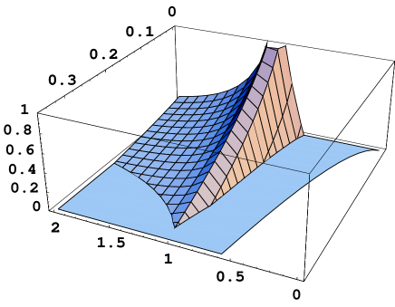
FIG. 5.: Gaussian maximized coherent information $Q_{G}(T)$ as function of $k$ and $N_{c}$. The shaded area is the area, where $Q_{\Theta}\geq 0$.

.

REFERENCES

- [1] C. H. Bennett, P. W. Shor, “Quantum information theory,” IEEE Trans. on Inform. Theory, IT-44, N6, pp. 2724-2742, 1998.
- [2] A. S. Holevo, “Coding theorems for Quantum Channels,” Tamagawa University Research Review, No.4, 1998. LANL Report no. quant-ph/9809023.
- [3] H. Barnum, M. A. Nielsen, B. Schumacher, “Information transmission through noisy quantum channels,” Phys. Rev. A, vol. A57, pp. 4153-4175, 1998. LANL Report no. quant-ph/9702049.
- [4] C. Adami and N. J. Cerf, “Capacity of noisy quantum channels,” Phys. Rev. A, vol. A56, pp. 3470-3485, 1997; LANL Report no. quant-ph/9609024.
- [5] H. Barnum, E. Knill, M. A. Nielsen, “On quantum fidelities and channel capacities,” LANL Report no. quant-ph/9809. To appear in IEEE Trans. on Inform. Theory.
- [6] C. H. Bennett, P. W. Shor, J. A. Smolin, A. V. Thapliyal, “Entanglement-assisted classical capacity of noisy quantum channel,” LANL Report no. quant-ph/9904023.
- [7] S. L. Braunstein, “Squeezing as an irreducible resource”, LANL Report no. quant-ph/9904002.
- [8] A. Furusawa, J. Sørensen, S. L. Braunstein, C. Fuchs, H. J. Kimble, E. S. Polzik, Science, vol.282, 706, 1998.
- [9] B. Demoen, P. Vanheuverzwijn, A. Verbeure, “Completely positive quasi-free maps on the CCR algebra,” Rep. Math. Phys., vol.15, pp. 27-39, 1979.
- [10] A. S. Holevo, “Some statistical problems for quantum Gaussian states,” IEEE Transactions on Information Theory, vol. IT-21, no.5, pp. 533-543, 1975.
- [11] A. S. Holevo, Probabilistic and statistical aspects of quantum theory, chapter 5, North-Holland, 1982.
- [12] R. F. Werner, “Quantum harmonic analysis on phase space,” J. Math. Phys., vol. 25, pp. 1404-1411, 1984.
- [13] A. S. Holevo, M. Sohma and O. Hirota, “The capacity of quantum Gaussian channels ,” Phys. Rev. A, vol. 59, N3, pp. 1820-1828, 1998.
- [14] A. S. Holevo, “Sending quantum information with Gaussian states,” LANL Report no. quant-ph/9809022. To appear in Proc. QCM-98, Ed. by M. D’Ariano, O.Hirota, P. Kumar.
- [15] A. S. Holevo, “Towards the mathematical theory of quantum communication channels,” Problems of Information Transm., vol. 8, no.1, pp. 63-71, 1972.
- [16] K. Kraus, States, effects and operations, Lect. Notes Phys., vol. 190, 1983.
- [17] G. Lindblad, “Quantum entropy and quantum measurements,” Lect. Notes Phys., vol. 378, Quantum Aspects of Optical Communication, Ed. by C. Benjaballah, O. Hirota, S. Reynaud, pp.71-80, 1991.
- [18] P. W. Shor et al, in preparation.
- [19] S. Lloyd, “The capacity of the noisy quantum channel,” Phys. Rev. A, vol. 56, pp. 1613, 1997.
- [20] D. P. DiVincenzo, P. W. Shor, J. A. Smolin, “Quantum-channel capacity of very noisy channels,” Phys. Rev. A, vol. 57, pp.830-839, 1998, LANL Report no. quant-ph/9706061.
- [21] V. I. Paulsen, Completely bounded maps and dilations, Longman Scientific and Technical 1986
- [22] D. Aharonov, A. Kitaev, and N. Nisan, “Quantum Circuits with Mixed States,” LANL Report no. quant-ph/9806029.
- [23] T. Ogawa, H. Nagaoka, “Strong converse to the quantum channel coding theorem,” LANL Report no. quant-ph/9808063 To appear in IEEE Trans. on Inform. Theory.
- [24] A. Winter, “Coding theorems and strong converse for quantum channels,” To appear in IEEE Trans. on Inform. Theory.
- [25] R. Simon, M. Selvadoray, G. S. Agarwal, “Gaussian states for finite number of bosonic degrees of freedom,” To appear in Phys. Rev..
- [26] C. W. Helstrom, Quantum detection and estimation theory, chapter 5, Academic press, 1976.
- [27] A. S. Holevo, “Generalized free states of the C∗-algebra of the CCR,” Theor. Math. Phys., vol. 6, no.1, pp. 3-20, 1971.
- [28] R.F. Werner, “The classical limit of quantum theory,” LANL Report no. quant-ph/9504016.