Two-photon Franson-type experiments and local realism

Abstract

The two-photon interferometric experiment proposed by Franson [Phys. Rev. Lett. 62, 2205 (1989)] is often treated as a “Bell test of local realism”. However, it has been suggested that this is incorrect due to the $50\%$ postselection performed even in the ideal gedanken version of the experiment. Here we present a simple local hidden variable model of the experiment that successfully explains the results obtained in usual realizations of the experiment, even with perfect detectors. Furthermore, we also show that there is no such model if the switching of the local phase settings is done at a rate determined by the internal geometry of the interferometers.

The two-particle interferometer introduced by Franson [5] has been used in many two-photon interferometric experiments [6, 7] that reveal complementarity between single and two-photon interference. The experiments cannot be described using standard methods involving classical electromagnetic fields [8]. However, the original paper was entitled Bell Inequality for Position and Time, and many subsequent papers claimed that the experiment constitutes a “Bell test of local realism involving time and energy”. Some authors were more skeptical that a true, unambiguous test of a Bell inequality was possible with these experiments, even in principle, since even the ideal gedanken model of the experiment requires a post-selection procedure in which $50\%$ of the events are discarded when computing the correlation functions [9, 10]. If all events are taken into account the Bell inequalities are not violated. Thus, a local hidden-variable (LHV) model is not ruled out, but even so, no LHV model for the experiment has yet been constructed [11].

The situation is further obscured by similar claims concerning certain other two-photon polarization experiments [12] where the problem of discarding $50\%$ of the events also appears [9, 13]. This was initially treated on equal footing with the problems of Franson-type experiments, but a recent analysis in [14] reestablishes the possibility of violating local realism. Unfortunately, that analysis cannot be adapted to the Franson experiment.

Our aim is to resolve this uncertainty. First, we shall construct a simple local realistic model for the usual operational realization of the experiment. Second, we shall prove that under the additional condition that the random changes of the state of the local interferometers are at a rate dictated by the internal geometry of the interferometers, no local hidden variable model exists for the perfect gedanken version of this type of experiment. Even then, the usual Bell inequality will be inadequate.

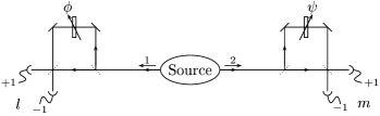
FIG. 1.: The generic setup of the Franson two-photon interference experiment.

Let us briefly describe the idea behind the Franson-type experiments (Fig. 1). The source yields photon pairs, correlated to within their coherence times, and the two photons are fed into two identical unbalanced Mach-Zehnder interferometers. The difference of the optical paths in those interferometers, $\Delta L$, satisfies the relation $\Delta L\gg cT_{\text{coh}}$, where $c$ is the speed of light and $T_{\text{coh}}$ is the coherence time of the photons. Such optical path differences prohibit any single-photon interference, so the single-photon probabilities are $\textstyle P(l|\phi)=P(m|\psi)=\frac{1}{2}$ (see Fig. 1). For the $50\%$ two-photon events that are coincident, one cannot distinguish between events where both photons take the long path and events where both take the short; hence, two-photon interference occurs:

$$P\bigl{(}l;m(\text{coinc.})|\phi,\psi\bigr{)}=\textstyle\frac{1}{8}\bigl{(}1+lm\cos(\phi+\psi)\bigr{)}.$$ (1)

For the other half of the two-photon events, one photon takes its short path and the other takes its long path, so that the registration times differ by $\Delta L/c$; there is consequently no interference because the events are distinguishable. One has $P(l_{\text{L}};m_{\text{E}}|\phi,\psi)=P(l_{\text{E}};m_{\text{L}}|\phi,\psi)=\textstyle\frac{1}{16}$, where E denotes the earlier count, and L denotes the later count. For future reference, we note that the local phase settings appearing in these formulas are those present when a photon in the long path is passing through the phase shifter, i.e., the phase setting at the actual detection time $t_{\text{d}}$, minus the time $t_{\text{ret}}$ it takes light to reach the detector from the location of the phase-shifter by the optical paths available within the interferometer.

Initially, the experiment is assumed to be performed in the following way. The usual locality condition is imposed, i.e., the local phase setting at one side does not affect the measurement result at the other side. Experimentally, this is enforced by switching the local phase settings on the time-scale $D/c$, where $D$ is the source–interferometer distance. We assume that $D\gg\Delta L$ [15]. The two experimenters (one at each side) record the $\pm 1$ counts, the detection times, and the appropriate values of the local phase settings. After the experiment is completed they perform a post-detection analysis on their recorded data, rejecting all pairs of events whose registration times differ by $\Delta L/c$. We now present a LHV model for the Franson experiment, valid in this experimental situation.

There are some general features that a LHV model of the experiment should have. The emission time should be one of the variables, because if the beamsplitters of, say, the right interferometer were removed, the photons would be detected solely by the detector $+1$, and the detection time $t_{\text{E}}$ would indicate the moment of emission. In this case, for any local setting of the phase $\phi$, the detections behind the left interferometer would either be coincident with the detections on the right side at $t_{E}$ (we shall call this an early detection), or delayed at $t_{\text{L}}=t_{\text{E}}+\Delta L/c$ (a late detection). This must be determined by the LHV model. Half of the events on the left side are early (E) and half are late (L). With the right interferometer in place, 1/4 of the events are early on the left and late on the right (EL), 1/4 are late on the left and early on the right (LE), and 1/2 are coincident. These coincident events must then consist of equal parts early-early (EE) and late-late (LL) events; no such distinction exists in the quantum description.

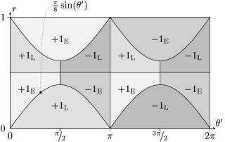
FIG. 2.: LHV model for detections at the left station. The shifted value of the angular hidden variable, $\theta^{\prime}=\theta-\phi$, and $r$, determine the result of the local observable, $l=\pm 1$, and whether the particle is detected early E or late L. The lower curve in the left side of the chart is given by $\frac{\pi}{8}\sin{\theta^{\prime}}$, and the shape of the other curves are of similar form.

In our model, the hidden variables are chosen to be an angular coordinate $\theta\in[0,2\pi]$ and an additional coordinate $r\in[0,1]$. The ensemble of hidden variables is chosen as that of a uniform distribution in this rectangle in $(\theta,r)$-space; each pair of particles is then described by a definite point $(\theta,r)$ in the rectangle, defined at the source at the moment of emission. At the left detector station, the measurement result is decided by the hidden variables $(\theta,r)$ and the local setting $\phi$ of the apparatus. When a photon arrives at the detection station, if the interferometer works properly [16] the variable $\theta$ is shifted by the current setting of the local phase shifter (i.e. $\theta^{\prime}=\theta-\phi$), and the result is read off Fig. 2. At the right detector station, a similar procedure is followed [16, 17]. In this case, the shift is to the value $\theta^{\prime\prime}=\theta+\psi$, and the result is obtained in Fig. 3 in the same manner as before.

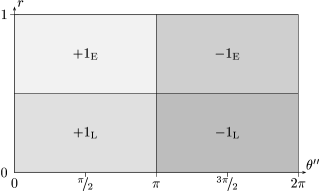
FIG. 3.: The measurement result at the right station given by the shifted hidden variables. The symbols have the same meaning as in Fig. 2.

The single-particle detection probabilities straightforwardly follow the quantum predictions, because in both Figs. 2 and 3, the total areas corresponding to $+1_{\text{E}}$, $-1_{\text{E}}$, $+1_{\text{L}}$, and $-1_{\text{L}}$ are all equal. The particle is equally likely to arrive early or late, and equally likely to go to the $+1$ or $-1$ output port of the interferometer. The coincidence probabilities are determined by interposing the two figures with the proper shifts.

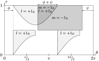
FIG. 4.: The shaded regions give the values for the initial hidden variables for which $l=+1_{\text{E}}$ or $m=-1_{\text{E}}$ are obtained (note that $\theta^{\prime}=\theta-\phi$ while $\theta^{\prime\prime}=\theta+\psi$). The overlap region of length $\phi+\psi$ represents the hidden variables for which both $l=+1_{\text{E}}$ and $m=-1_{\text{E}}$ are obtained.

For example, the probability of having $l=+1_{\text{E}}$ and $m=-1_{\text{E}}$ simultaneously is the area of the set indicated in Fig. 4 divided by $2\pi$ (the total area is $2\pi$ whereas the total probability is 1). The net coincidence probability is

$$P\bigl{(}+1;-1(\text{coinc.})|\phi,\psi\bigr{)}$$ (2)

$$\qquad=P(+1_{\text{E}};-1_{\text{E}}|\phi,\psi)+P(+1_{\text{L}};-1_{\text{L}}|\phi,\psi)$$ (3)

$$\qquad=\frac{2}{2\pi}\int_{0}^{\phi+\psi}\frac{\pi}{8}\sin(\theta)d\theta=\frac{1}{8}\bigl{(}1-\cos{(\phi+\psi)}\bigr{)}.$$ (4)

It is easy to verify that this model also gives the correct prediction for the other detection events.

Somewhat remarkably, the above construction implies that the Franson experiment does not and cannot violate local realism if one disregards the fact that the unbalanced Mach-Zehnder interferometers are extended objects. The reason that this construction is possible is that the $50\%$ post-selection procedure discussed above may yield an ensemble of detected pairs that depends on the phase settings (rendering the Bell inequality useless [18]). However, we shall now show that if the phase switching is performed at the time-scale $\Delta L/c$, typical for retardations within the interferometers, there is no LHV description of the experiment. In particular, we will describe an experimental procedure that allows us to post-select an unchanging part of the LHV ensemble, thus reenabling the Bell inequality on this part of the ensemble.

Let us look at one interferometer as an extended object to establish what would take place if local realism were to hold. In the interferometer, the decision of a detection to occur early (at $t_{\text{E}}$) or late (delayed by $\Delta L/c$) cannot be made later than the time $t_{\text{E}}$. This decision is based on the local variables and the properly retarded phase setting. No phase setting after $t_{\text{E}}-t_{\text{ret}}$ can causally affect this E/L choice [19]. The choice $\pm 1$ is also based on the local variables and the properly retarded phase setting at the interferometer in question, but this choice may be made as late as the detection time $t_{\text{d}}$ ($t_{\text{d}}=t_{\text{E}}$ for early events or $t_{\text{d}}=t_{\text{L}}\equiv t_{\text{E}}+\Delta L/c$ for late). Therefore, in the case of a late detection, the choice E/L and the choice $\pm 1$ can be made at different times ($t_{\text{E}}$ and $t_{\text{L}}$, respectively) based on possibly different phase settings.

Looking at only one interferometer, it is not possible to discern early detections from late ones, so an experimenter at that interferometer knows only the result $\pm 1$, the detection time $t_{\text{d}}$, and two possibly different phase settings at $t_{\text{d}}-\Delta L/c-t_{\text{ret}}$ and $t_{\text{d}}-t_{\text{ret}}$. She also knows that for the events that are late, the later of these two phase settings cannot causally have affected the E/L decision, so the hypothetical late subensemble does not depend on the phase setting at $t_{\text{d}}-t_{\text{ret}}$ but only on the phase setting at the earlier time $t_{\text{d}}-\Delta L/c-t_{\text{ret}}$. By rejecting events where the phase setting at $t_{\text{d}}-\Delta L/c-t_{\text{ret}}$ does not have a certain value ($\phi_{0}$, say), she ensures that the late subensemble does not change at all. To allow for settings other than $\phi_{0}$ at the later decision time, a device which switches fast (on the time-scale $\Delta L/c$) and randomly between phase settings is needed [20].

Thus, in the modified full experiment both experimenters should use fast devices that randomly switch between the phase settings $\phi_{0}$, $\phi_{1}$, $\ldots$, $\phi_{N}$ on the left side and $\psi_{0}$, $\psi_{1}$, $\ldots$, $\psi_{N}$ on the right. They record the appropriate data and reject (a) pairs of events whose registration times differ by $\Delta L/c$ and (b) pairs of events which do not have the feature that the phase setting at $t_{\text{d}}-\Delta L/c-t_{\text{ret}}$ was $\phi_{0}$ on the left and $\psi_{0}$ on the right. The latter event rejection ensures that the hypothetical LL subensemble within the remaining data is independent of the phase settings at $t_{\text{d}}-t_{\text{ret}}$. Then, if local realism holds, the Bell-CHSH inequality applies to this LL subensemble,

$$|E_{\text{L}\text{L}}(\phi_{1},\psi_{1})+E_{\text{L}\text{L}}(\phi_{2},\psi_{1})|$$ (5)

$$+|E_{\text{L}\text{L}}(\phi_{2},\psi_{2})-E_{\text{L}\text{L}}(\phi_{1},\psi_{2})|\leq 2,$$ (6)

where the phases are taken at $t_{\text{d}}-t_{\text{ret}}$, and $E_{\text{L}\text{L}}(\phi,\psi)$ denotes the Bell-type conditional correlation function on the remaining LL subensemble. This is valid only because each of the correlation functions above is an average on the same ensemble. Had the ensemble depended on the phase settings at $t_{\text{d}}-t_{\text{ret}}$, the bound would have been higher.

Indeed, the remaining EE subensemble may still depend on the phase setting at $t_{\text{d}}-t_{\text{ret}}$ even after this selection, and we only have

$$|E_{\text{E}\text{E}}(\phi,\psi)|\leq 1.$$ (7)

Experimentally, this “noise” in form of EE events cannot be distinguished from the LL events. Of all events that survive the described selection, again half are EE and half are LL, so that

$$E_{\text{coinc.}}(\phi,\psi)=\frac{1}{2}E_{\text{L}\text{L}}(\phi,\psi)+\frac{1}{2}E_{\text{E}\text{E}}(\phi,\psi).$$ (8)

Thus, a modified Bell-CHSH inequality valid for all the coincident events is implied by (6)–(8), namely

$$|E_{\text{coinc.}}(\phi_{1},\psi_{1})+E_{\text{coinc.}}(\phi_{2},\psi_{1})|$$ (9)

$$+|E_{\text{coinc.}}(\phi_{2},\psi_{2})-E_{\text{coinc.}}(\phi_{1},\psi_{2})|\textstyle\leq\frac{1}{2}(2+4)=3.$$ (10)

Unfortunately, this inequality is not violated by the conditional quantum correlation function $E_{\text{coinc.}}^{\text{QM}}(\phi,\psi)=\cos{(\phi+\psi)}$ which yields a maximum of $2\sqrt{2}$. However, a violation may be obtained by a “chained” extension of the Bell-CHSH inequality (see Ref. [21]):

$$|E_{\text{L}\text{L}}(\phi_{1},\psi_{1})+E_{\text{L}\text{L}}(\phi_{2},\psi_{1})|$$ (11)

$$+|E_{\text{L}\text{L}}(\phi_{2},\psi_{2})+E_{\text{L}\text{L}}(\phi_{3},\psi_{2})|$$ (12)

$$+|E_{\text{L}\text{L}}(\phi_{3},\psi_{3})-E_{\text{L}\text{L}}(\phi_{1},\psi_{3})|\leq 4.$$ (13)

If local realism holds, (7), (8), and (13) yield

$$|E_{\text{coinc.}}(\phi_{1},\psi_{1})+E_{\text{coinc.}}(\phi_{2},\psi_{1})|$$ (14)

$$+|E_{\text{coinc.}}(\phi_{2},\psi_{2})+E_{\text{coinc.}}(\phi_{3},\psi_{2})|$$ (15)

$$+|E_{\text{coinc.}}(\phi_{3},\psi_{3})-E_{\text{coinc.}}(\phi_{1},\psi_{3})|\leq\textstyle\frac{1}{2}(4+6)=5.$$ (16)

This inequality is violated by quantum predictions, e.g., at $\phi_{1}=0$, $\phi_{2}=-\pi/3$, $\phi_{3}=-2\pi/3$, $\psi_{1}=\pi/6$, $\psi_{2}=\pi/2$, and $\psi_{3}=5\pi/6$ we obtain

$$5\cos(\pi/6)-\cos(5\pi/6)=6\cos(\pi/6)\approx 5.20>5.$$ (17)

In conclusion, to obtain a violation of local realism in an experiment one needs random fast switching and a filtering of the hypothetical late-late subensemble so that this ensemble does not depend on the phase settings [20]. Even then, the standard Bell inequalities are not sensitive enough to show a violation of local realism in the experiment, because their bound is raised by the “noise” introduced by the early-early subensemble. However, a “chained Bell inequality” may be used, which is violated even with this “noise” included.

The reported violations of local realism from Franson experiments have to be reexamined. While the results formally violate the standard Bell-CHSH inequality, the inequality is not applicable. The inequality (16) is applicable, but when using it, one should note that it is violated only if the visibility is more than $5/5.2\approx 96\%$. This is significantly higher than the usual $71\%$ bound discussed in the reported experiments [6, 7].

It has been proposed that entangled photons can be used to perform quantum cryptography [22]; specifically, the Franson-type experiment has been discussed in this context [7]. In such schemes security checks can be performed by testing whether the signals violate the Bell inequalities. It remains a subtle question if the link to local realism is important for this kind of security check; if so, the Bell-CHSH inequality is not appropriate for the Franson setup.

Sven Aerts acknowledges a grant by the Flemish Institute for the Advancement of Scientific-Technological Research in the Industry (IWT). Jan-Åke Larsson has received partial support from the Swedish Natural Science Research Council. Marek Żukowski was supported by the Flemish-Polish Scientific Collaboration Program No. 007, by UG Program BW/5400-5-0264-9, and also acknowledges discussions with E. Santos, H. Weinfurter and A. Zeilinger.

REFERENCES

- [1] Electronic address: saerts@vub.ac.be
- [2] Electronic address: kwiat@lanl.gov
- [3] Electronic address: jalar@mai.liu.se
- Γ[278] Electronic address: fizmz@univ.gda.pl
- [5] J. D. Franson, Phys. Rev. Lett. 62, 2205 (1989). We are not interested here in modifications of Franson’s idea like those in D. V. Strekalov, T. B. Pittman, A. V. Sergienko, Y. H. Shih and P. G. Kwiat, Phys. Rev. A 54, R1 (1996).
- [6] P. G. Kwiat, W. A. Vareka, C. K. Hong, H. Nathel and R. Y. Chiao, Phys. Rev. A 41, 2910 (1990); Z. Y. Ou, X. Y. Zou, L. J. Wang and L. Mandel, Phys. Rev. Lett. 65, 321 (1990). The first experiment with high time resolution is by J. Brendel, E. Mohler and W. Martiensen, Phys. Rev. Lett. 66, 1142 (1991), however their arrangement involved Michelson interferometers. The first full realization seems to be in P. G. Kwiat, A. M. Steinberg and R. Y. Chiao, Phys. Rev. A 47, R2472 (1993).
- [7] P. R. Tapster, J. G. Rarity, and P. C. M. Owens, Phys. Rev. Lett., 73, 1923 (1994), W. Tittel, J. Brendel, H. Zbinden, and N. Gisin, ibid. 81, 3563 (1998).
- [8] J. D. Franson, Phys. Rev. Lett. 67, 290 (1991); Z. Y. Ou and L. Mandel, J. Opt. Soc. Am. B 7, 2127 (1990).
- [9] L. De Caro and A. Garuccio, Phys. Rev. A 50, R2803 (1994).
- [10] P. G. Kwiat, Phys. Rev. A 52, 3380 (1995).
- [11] The LHV model of E. Santos [Phys. Lett. A 212, 10 (1996)] is limited to detection efficiency lower than .
- [12] Z. Y. Ou and L. Mandel, Phys. Rev. Lett. 61, 50 (1988); Y. H. Shih and C. O. Alley, ibid. 61 2921 (1988).
- [13] P. G. Kwiat, P. H. Eberhard, A. M. Steinberg and R. Y. Ciao, Phys. Rev. A 49, 3209 (1994).
- [14] S. Popescu, L. Hardy and M. Żukowski, Phys. Rev. A., 56, R4353 (1997).
- [15] The model does not take into account the fact that the local interferometer and the detection station are extended objects. This is reasonable, provided the state of the interferometer does not undergo rapid changes at the time scale .
- [16] In case the interferometer is dismantled, the detection is always . If one path is blocked, the events are randomly chosen from or each with probability 1/4 (early or late as appropriate), or “no detection” with probability 1/2. A modification of this type may be made as long as the assumption in [15] is valid.
- [17] The model can be trivially symmetrized.
- [18] J.-Å. Larsson, Phys. Rev. A, 57 3304 (1998).
- [19] The proper retardation for the E/L choice is really along the shortest phase-switch–detector path (not the optical path). It is possible to arrange the experiment so the two are roughly of the same size, and our argument still holds.
- [20] Given that the switching is fast (on the time-scale ) and random, it is possible to prove the inequalities even without this filtering on the late ensemble.
- [21] P. M. Pearle, Phys. Rev. D 2, 1418 (1970); A. Garuccio and F. Selleri, Found. Phys. 10, 209 (1980); S. L. Braunstein and C. M. Caves, Proc. 3rd Int. Symp. on Foundations of quantum mechanics, eds. S Kobayashi et al, (Phys. Soc. Japan, Tokyo 1989).
- [22] A. K. Ekert (1991), Phys. Rev. Lett. 67, 661.