Continuous Spectra of Generalized Kronig-Penney Model

Abstract

The standard Kronig-Penney model with periodic $\delta$ potentials is extended to the cases with generalized contact interactions. The eigen equation which determines the dispersion relation for one-dimensional periodic array of the generalized contact interactions is deduced with the transfer matrix formalism. Numerical results are presented which reveal unexpected band spectra with broader band gap in higher energy region for generic model with generalized contact interaction.

I Introduction

The contact interaction occupies a special position in quantum mechanics. The system with contact interaction is often rigorously solvable AG88 , and also is useful in examining the effect of small obstacle on particle motion. The first influential work on contact interactions was done by Kronig and Penney KP31 . The model, which has potential consisting of a periodic array of $\delta$ functions, has been widely regarded as a standard reference model in the solid-state physics for more than half a century.

In spite of the seeming simplicity of contact interactions, there are several non-trivial aspects which are largely left unexplored. Even in the simplest setting of one dimension, there has been a historically longstanding problem of realizing the generalized contact interaction in the small-size limit of a local self-adjoint interaction. In one dimension, there are a four-parameter family of generalized contact interactions which conserve the current at both sides of the interaction GK85 . This corresponds to the fact that the one-dimensional kinetic energy operator $T=-\frac{d^{2}}{dx^{2}}$ with domain $C^{\infty}_{0}({\bf R}\backslash\{0\})$ has deficiency indices $(2,2)$ AG88 . In non-relativistic formalism, the current operator is given by

$$j(x)={\bf\Psi}^{\dagger}(x)\sigma_{2}{\bf\Psi}(x),$$ (1)

where ${\bf\Psi}$ is defined in terms of the wave function $\varphi$ and its space derivative as

$${\bf\Psi}(x)=\left(\begin{array}[]{c}\varphi(x)\\ \frac{1}{2m}\varphi^{\prime}(x)\end{array}\right).$$ (4)

The matrix $\sigma_{2}$ in Eq.(1) is the second component of Pauli matrices;

$$\sigma_{2}=\left(\begin{array}[]{cc}0&-i\\ i&0\end{array}\right).$$ (7)

In Eq.(4), $m$ is the mass of a particle. If we put a contact interaction at $x=0$, the connection of ${\bf\Psi}$ between both sides of the origin can be characterized by

$${\bf\Psi}(+0)={\cal V}{\bf\Psi}(-0),$$ (8)

where the current conservation $j(+0)=j(-0)$ requires

$${\cal V}^{\dagger}\sigma_{2}{\cal V}=\sigma_{2}.$$ (9)

The generic solution of Eq.(9) is given by

$${\cal V}=e^{i\theta}\left(\begin{array}[]{cc}\gamma&\delta\\ \beta&\alpha\end{array}\right),$$ (12)

where $\theta\in{\bf R}$ and $\alpha\gamma-\beta\delta=1$. The condition (12) covers a four-parameter family. (See AD98 ; CF01 ; TF01 for the discussions on rigorous characterization of the full parameter space.) In addition to the usual $\delta$ potential

$${\cal V}_{\delta}(v)=\left(\begin{array}[]{cc}1&0\\ v&1\end{array}\right),$$ (15)

this family includes the so-called $\varepsilon$ potential (also known by a misnomer, $\delta^{\prime}$ potential). The $\varepsilon$ potential induces such a boundary condition that the wave function has continuous first derivative on the right and left, but it has a jump proportional to the first derivative S86b ;

$${\cal V}_{\varepsilon}(u)=\left(\begin{array}[]{cc}1&u\\ 0&1\end{array}\right).$$ (18)

In CS98a , we have constructed the $\varepsilon$ potential in the small distance limit of three nearby $\delta$ potentials and realized in terms of usual $\delta$ and $\varepsilon$ potentials a three-parameter family of self-adjoint extensions under the assumption of time reversal symmetry. This treatment have been generalized with finite range potential with double short-range limit with different scales ENZ01 . Also, the relativistic origin of $\varepsilon$ potential has been discussed in SM99a . Contrary to the general belief, some of the non-$\delta$ contact interactions appears in realizable settings in quite a natural manner BBM95 , and, in fact, they are essential in understanding the nature of one-dimensional many-body system CS99 .

In light of these facts, it is quite interesting to examine the nature of one-dimensional system with a periodic array of generalized contact interactions. For this purpose, we generalize the Kronig-Penney model to the cases of generalized point interactions. We are particularly interested in the question whether the original Kronig-Penney model with $\delta$-interaction is a generic zero-range limit of more realistic models with finite-range interactions. In this paper, we assume that the system has time-reversal symmetry. In this case, we have $\theta=0$ in Eq.(12), hence

$${\cal V}=\left(\begin{array}[]{cc}\gamma&\delta\\ \beta&\alpha\end{array}\right)\in SL(2,{\bf R}).$$ (21)

After giving the formulation of the generalized Kronig-Penney model with generic contact interactions in Sect.2, some elementary numerical results are presented in Sect.3. It will be shown that the standard periodic array of $\delta$ potentials has a specific band structure, compared to the generic cases; The band gap tends to disappear in the high energy limit for periodic $\delta$ array, while the band width becomes narrower for higher bands in generic cases. The current work is summarized in Sect.4.

II Formalism

We consider a one-dimensional periodic array of a generalized contact interaction, the connection condition of which is described by ${\cal V}$ in Eq.(21). We assume that the interactions are located at $x=na$, ($n=0,\pm 1,\pm 2,\cdots$). Here we denote the lattice interval by $a$. The assumed potential is shown in Fig.1.

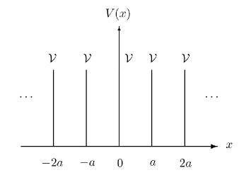
Figure 1: Periodic potential of Kronig-Penny model with generalized contact interaction. The two-by-two matrix ${\cal V}\in SL(2,{\bf R})$ represents the connection condition at each interaction in the transfer matrix formalism.

Schrödinger equation is given by

$$-\frac{1}{2m}\varphi^{\prime\prime}(x)=E\varphi(x),\ \ (x\neq na)$$ (22)

with the boundary condition

$${\bf\Psi}(na+0)={\cal V}{\bf\Psi}(na-0)$$ (23)

at $x=na$. In the transfer matrix formalism, Eq.(22) is written as the first-order coupled equation;

$${\bf\Psi}^{\prime}(x)={\cal H}{\bf\Psi}(x),\ \ (x\neq na),$$ (24)

where we define

$${\cal H}=\left(\begin{array}[]{cc}0&2m\\ -\frac{k_{0}^{2}}{2m}&0\end{array}\right)$$ (27)

with $k_{0}=\sqrt{2mE}$. The solution of Eq.(24) is written as

$${\bf\Psi}(x)={\cal G}(x-x_{0}){\bf\Psi}(x_{0})$$ (28)

by using the exponential function of ${\cal H}x$;

$${\cal G}(x)\equiv e^{{\cal H}x}=\cos(k_{0}x)I_{2}+\frac{\sin(k_{0}x)}{k_{0}}{\cal H}.$$ (29)

Here we assume $na\notin[x_{0},x]$ in Eq.(28). In Eq.(29), $I_{2}$ is the two-by-two identity matrix. Note that $\det{\cal G}(x)=1$ because of $Tr{\cal H}=0$.

We can see

$${\cal G}(x){\bf u}_{\pm k_{0}}=e^{\pm ik_{0}x}{\bf u}_{\pm k_{0}}$$ (30)

with

$${\bf u}_{\pm k_{0}}=\frac{1}{\sqrt{2}}\left(\begin{array}[]{c}1\\ \pm i\frac{k_{0}}{2m}\end{array}\right).$$ (33)

Namely, ${\cal G}(x)$ has eigenvalues $e^{\pm ik_{0}x}$ with the associated eigenfunction ${\bf u}_{\pm k_{0}}$ in Eq.(33). Also the complex conjugate of ${\cal G}(x)$ satisfies

$${\cal G}^{\dagger}(x){\bf v}_{\pm k_{0}}=e^{\mp ik_{0}x}{\bf v}_{\pm k_{0}}$$ (34)

with

$${\bf v}_{\pm k_{0}}=\frac{1}{\sqrt{2}}\left(\begin{array}[]{c}1\\ \pm i\frac{2m}{k_{0}}\end{array}\right).$$ (37)

That is, ${\cal G}^{\dagger}(x)$ has eigenvalues $e^{\mp ik_{0}x}$ with the associated eigenfunction ${\bf v}_{\pm k_{0}}$ in Eq.(37). The eigenfunctions ${\bf u}_{\pm k_{0}}$ and ${\bf v}_{\pm k_{0}}$ satisfy the bi-orthogonal relations;

$${\bf v}_{\pm k_{0}}^{\dagger}{\bf u}_{\pm k_{0}}=1,\hskip 12.91663pt{\bf v}_{\mp k_{0}}^{\dagger}{\bf u}_{\pm k_{0}}=0.$$ (38)

By Bloch theorem, we can set

$$\varphi(x)=e^{ikx}u(x),\ \ \ \ (k\in{\bf R})$$ (39)

in Eq.(22), where the function $u$ has period $a$;

$$u(x+a)=u(x).$$ (40)

Since

$$\varphi^{\prime}(x) = e^{ikx}(u^{\prime}(x)+iku(x)),$$ (41)

$$\varphi^{\prime\prime}(x) = e^{ikx}(u^{\prime\prime}(x)+2iku^{\prime}(x)-k^{2}u(x)),$$ (42)

we obtain the equation for $u$;

$$-u^{\prime\prime}(x)-2iku^{\prime}(x)+k^{2}u(x)=k_{0}^{2}u(x),$$ (43)

($x\neq na$). In the vector notation

$${\bf\tilde{\Psi}}(x)=\left(\begin{array}[]{c}u(x)\\ \frac{1}{2m}u^{\prime}(x)\end{array}\right),$$ (46)

we rewrite Eq.(43) as

$${\bf\tilde{\Psi}}^{\prime}(x)={\tilde{\cal H}}{\bf\tilde{\Psi}}(x),\hskip 12.91663pt(x\neq na)$$ (47)

with

$${\tilde{\cal H}}=\left(\begin{array}[]{cc}0&2m\\ \frac{k^{2}-k_{0}^{2}}{2m}&-2ik\\ \end{array}\right).$$ (50)

It is clear from Eqs.(39) and (41) that the two vectors ${\bf\Psi}(x)$ and ${\bf\tilde{\Psi}}(x)$ are related by

$${\bf\Psi}(x)={\cal M}{\bf\tilde{\Psi}}(x)$$ (51)

with

$${\cal M}=e^{ikx}\left(\begin{array}[]{cc}1&0\\ \frac{ik}{2m}&1\end{array}\right).$$ (54)

The solution of Eq.(47) is given by

$${\bf\tilde{\Psi}}(x)={\tilde{\cal G}}(x-x_{0}){\bf\tilde{\Psi}}(x_{0}),$$ (55)

where ${\tilde{\cal G}}(x)$ is the exponential function of ${\tilde{\cal H}}x$;

$${\tilde{\cal G}}(x)$$

$$= \!\!e^{{\tilde{\cal H}}x}$$

$$= \!\!e^{-ikx}\left[{\cos(k_{0}x)I_{2}+\frac{\sin(k_{0}x)}{k_{0}}\left(\begin{array}[]{cc}ik&2m\\ \frac{k^{2}-k_{0}^{2}}{2m}&-ik\\ \end{array}\right)}\right].$$ (59)

Here we assume $na\notin[x_{0},x]$. Since $Tr{\tilde{\cal H}}=-2ik$, we have $\det{\tilde{\cal G}}(x)=e^{(Tr{\tilde{\cal H}})x}=e^{-2ikx}$. It is seen from Eqs.(23) and (51) that the connection condition for ${\bf\tilde{\Psi}}$ at $x=na$ is given by

$${\bf\tilde{\Psi}}(na+0)={\tilde{\cal V}}{\bf\tilde{\Psi}}(na-0)$$ (60)

with

$${\tilde{\cal V}} = {\cal M}^{-1}{\cal V}{\cal M}$$ (65)

$$= \left(\begin{array}[]{cc}1&0\\ -\frac{ik}{2m}&1\end{array}\right){\cal V}\left(\begin{array}[]{cc}1&0\\ \frac{ik}{2m}&1\end{array}\right).$$

Note that $\det{\tilde{\cal V}}=\det{\cal V}=1$. The periodicity for $u$ in Eq.(40) is equivalent to

$${\bf\tilde{\Psi}}(x+a)={\bf\tilde{\Psi}}(x).$$ (66)

In particular, with $x=na-0$, we have

$${\tilde{\cal G}}(a){\tilde{\cal V}}{\bf\tilde{\Psi}}(na-0)={\bf\tilde{\Psi}}(na-0),$$ (67)

since

$${\bf\tilde{\Psi}}((n+1)a-0) = {\tilde{\cal G}}(a){\bf\tilde{\Psi}}(na+0)$$ (68)

$$= {\tilde{\cal G}}(a){\tilde{\cal V}}{\bf\tilde{\Psi}}(na-0).$$

Eq.(67) requires the two-by-two matrix ${\tilde{\cal G}}(a){\tilde{\cal V}}$ has eigenvalue $1$:

$$\det(I_{2}-{\tilde{\cal G}}(a){\tilde{\cal V}})=0.$$ (69)

Since $\det({\tilde{\cal G}}(a){\tilde{\cal V}})=\det{\tilde{\cal G}}(a)=e^{-2ika}$, the other eigenvalue of the matrix ${\tilde{\cal G}}(a){\tilde{\cal V}}$ should be $e^{-2ika}$. This indicates

$$Tr({\tilde{\cal G}}(a){\tilde{\cal V}})=1+e^{-2ika}.$$ (70)

A simple matrix calculation shows

$$M\tilde{{\cal H}}M^{-1}=-ikI_{2}+{\cal H},$$ (71)

which gives the relation between $\tilde{\cal{G}}(x)$ and ${\cal G}(x)$;

$$M\tilde{\cal{G}}(x)M^{-1}=e^{M\tilde{{\cal H}}M^{-1}x}=e^{-ikx}{\cal G}(x).$$ (72)

From Eq.(72), we obtain

$${\tilde{\cal G}}(a){\tilde{\cal V}}=e^{-ika}{\cal M}^{-1}{\cal G}(a){\cal V}{\cal M}.$$ (73)

Thus we conclude that the condition (70) is equivalent to

$$Tr({\cal G}(a){\cal V})=2\cos(ka).$$ (74)

Eq.(74) determines the dispersion relation for a periodic array of the generalized contact interaction characterized by the connection condition (21). Inserting Eqs.(21) and (29) into Eq.(74), we obtain the eigenvalue equation

$$(\alpha+\gamma)\cos(k_{0}a)+\sin(k_{0}a)\left(\frac{2m}{k_{0}}\beta-\frac{k_{0}}{2m}\delta\right)$$

$$=2\cos(ka).$$ (75)

III Numerical Examples

In this section, we give numerical examples of the band spectrum in several cases; the usual periodic $\delta$, periodic $\varepsilon$ as well as periodic array with some typical one-parameter families of generic contact interactions. It will be shown that the band structure of periodic $\delta$ potential is not generic; The band width becomes broader even in the $k$ (wave number) space for $\delta$ array as the energy increases, contrary to the generic cases. Throughout this section, we take the mass of particle $m=1/2$ and the lattice interval $a=1$ in numerical calculations.

Let us begin with the periodic $\delta$ potentials. From Eq.(II) together with Eq.(15), we obtain the eigenvalue equation for $\delta$ array;

$$\cos(k_{0})+\frac{v\sin(k_{0})}{2k_{0}}=\cos(k),$$ (76)

where $v$ is the strength of each $\delta$. Eq.(76) is the well-known result in the standard Kronig-Penney model. Fig.2(a) shows the band spectrum as a function of $v$. With the parameters $v$ and $E=k_{0}^{2}$ in the shaded region, the equation (76) has the solution $k$. The condition for the existence of the solution is given by

$$\left|\cos(k_{0})+\frac{v\sin(k_{0})}{2k_{0}}\right|\leq 1.$$ (77)

For $v=0$, one sees the continuous spectrum for positive energy and there is no bound states, as expected.

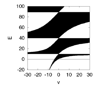
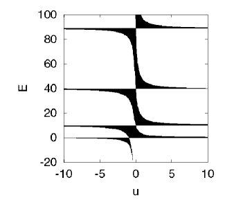
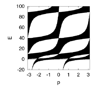
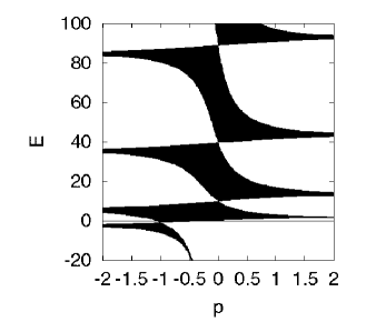
Figure 2: Band spectrum for a periodic array of generalized contact interaction characterized by one-parameter family of connection conditions; Eqs.(7), (8), (49), and (51) in (a), (b), (c), and (d), respectively. In all cases, the horizontal axis is the parameter associated with each family, while the vertical axis is the energy $E=\frac{k_{0}^{2}}{2m}$. The mass is set to $m=1/2$. The lattice interval is set to $a=1$.

For $v\neq 0$, the band structure appears and the band width becomes narrower as the strength $|v|$ increases. In the limit of $|v|\longrightarrow\infty$, one obtains point spectrum $E=(n\pi)^{2}$. For negative $v$, there is a negative energy band which goes to the minus infinity in the limit of $v\longrightarrow-\infty$. In both limits $v\longrightarrow\pm\infty$, the boundary condition around each $\delta$ corresponds to the so-called separated boundary condition. Each region between two neighboring $\delta$’s are separated from the other regions and the wave function satisfies the Dirichlet boundary condition such that it vanishes at each $\delta$.

For $\varepsilon$ potential of strength $u$, we obtain the eigenvalue equation

$$\cos(k_{0})-\frac{uk_{0}\sin(k_{0})}{2}=\cos(k).$$ (78)

Fig.2(b) shows the band spectrum as a function of $u$. The condition for the existence of the solution is given by

$$\left|\cos(k_{0})-\frac{uk_{0}\sin(k_{0})}{2}\right|\leq 1.$$ (79)

The case of $u=0$ corresponds to the free space. For $u\neq 0$, the band structure appears and the band width becomes rapidly narrower as the strength $|u|$ increases. In the limit of $|u|\longrightarrow\infty$, one obtains point spectrum $E=(n\pi)^{2}$. In this limit, each region between two neighboring $\varepsilon$’s are separated from the other regions and the wave function satisfies the Neumann boundary condition such that its derivative vanishes at each $\varepsilon$. For negative $u$, there is a negative energy band which goes to the minus infinity in the limit of $u\longrightarrow-0$.

To see the generic cases, we show in Fig2.(c) the band spectrum for the one-parameter family of the connection condition;

$${\cal V}=\left(\begin{array}[]{cc}\cos p&-\sin p\\ \sin p&\cos p\end{array}\right),\ \ \ (-\pi<p\leq\pi).$$ (82)

The band spectrum is determined by

$$\left|\cos(p)\cos(k_{0})+\frac{\sin(p)\sin(k_{0})}{2}\left(k_{0}+\frac{1}{k_{0}}\right)\right|\leq 1.$$ (83)

With $p\neq 0,\pi$, we see the band structure as in other generic cases. The band spectrum has period $\pi$, as seen from Eq.(83) and the energy spectrum for $p=\pi$ is the same as in the free space ($p=0$). However, the wave function for $p=\pi$ differs from the free one. Indeed, it has the same amplitude as the continuous wave function in the free space, but it changes the phase and as a result it is discontinuous at each obstacle. Such “duality” of $p=0$ and $p=\pi$ induces double spiral structure in energy spectrum C98 , as implied in Fig.2(c).

Fig.2(d) shows the case for the one-parameter family of

$${\cal V}=\left(\begin{array}[]{cc}\cosh p&\sinh p\\ \sinh p&\cosh p\end{array}\right),\ \ \ (p\in{\bf R}).$$ (86)

In this case, the band spectrum is determined by

$$\left|\cosh(p)\cos(k_{0})-\frac{\sinh(p)\sin(k_{0})}{2}\left(k_{0}-\frac{1}{k_{0}}\right)\right|\leq 1.$$ (87)

As in other cases, the band width becomes gradually narrower, as the perturbation becomes larger.

An important point is that the $\delta$ potential, among generic point interactions, has rather a special energy dependence of band structure. To see this, we show the band spectrum including higher energy region in Figs.3(a)-(d), which correspond to Figs.2(a)-(d), respectively. In Fig.3, the vertical axis is the wave number $k_{0}$, instead of the energy $E$, which is suitable for our present purpose, since the state density is constant [of $O(k^{0})$] in one dimension. One can see that in generic cases including $\varepsilon$, the band width becomes narrower for higher bands, while the band gap tends to disappear for $\delta$ array.

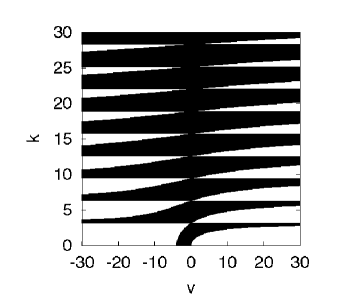
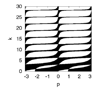
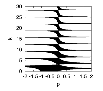
Figure 3: The energy dependence of the band spectrum. The indications are the same as in Fig.2 except that the vertical axis is the wave number $k_{0}$.

The reason is easy to understand by examining the scattering properties by a single contact interaction.

In the transfer matrix formulation, the bi-orthogonal eigenvectors (33) and (37) serve to examine the scattering properties. Since $e^{\pm ik_{0}x}{\bf u}_{\pm k_{0}}$ are the solutions of the equation (24), the wave function is written as

$${\bf\Psi}(x)=\left\{\begin{array}[]{ll}e^{ik_{0}x}{\bf u}_{+k_{0}}+R_{S}e^{-ik_{0}x}{\bf u}_{-k_{0}},&(x<0),\\ T_{S}e^{ik_{0}x}{\bf u}_{+k_{0}},&(x>0),\\ \end{array}\right.$$ (90)

where $T_{S}$ and $R_{S}$ are transmission and reflection coefficients, respectively. We assume that the contact interaction is placed at $x=0$ and the incident wave comes from minus infinity in Eq.(90). From the connection condition (8), we obtain

$$T{\bf u}_{+k_{0}}={\cal V}({\bf u}_{+k_{0}}+R_{S}{\bf u}_{-k_{0}}).$$ (91)

Multiplying ${\bf v}_{+k_{0}}^{\dagger}{\cal V}^{-1}$ from the left and using the bi-orthogonal relations (38), we can estimate the transition probability as

$$|T|^{2} = \left|{\bf v}_{+k_{0}}^{\dagger}{\cal V}^{-1}{\bf u}_{+k_{0}}\right|^{-2}$$ (92)

$$= 4\left[\alpha^{2}+\gamma^{2}+2+\delta^{2}\frac{k_{0}^{2}}{4m^{2}}+\beta^{2}\frac{4m^{2}}{k_{0}^{2}}\right]^{-1}.$$

The reflection probability is given by

$$|R|^{2}=1-|T|^{2}.$$ (93)

Eq.(92) shows $|T|^{2}\longrightarrow 0$ as $k_{0}\longrightarrow+\infty$, namely perfect reflection in the high energy limit for generic cases. The exception arises in case of $\delta=0$, namely $\delta$ potential. In this case, we have

$$|T_{\delta}|^{2} = \left[1+\frac{v^{2}m^{2}}{k_{0}^{2}}\right]^{-1},$$ (94)

$$|R_{\delta}|^{2} = \left[1+\frac{k_{0}^{2}}{v^{2}m^{2}}\right]^{-1}.$$ (95)

Thus, $|T_{\delta}|^{2}\longrightarrow 1$ as $k_{0}\longrightarrow+\infty$, namely perfect transmission is realized. This explains why the band width broadens even in the $k_{0}$ (wave number) space for the $\delta$ array as the energy increases and the band gap disappears in the high energy limit.

In the low energy limit, the $\varepsilon$ potential rather than $\delta$ shows a special nature. From Eqs.(92) and (93), one recognizes in generic cases, $|T|^{2}\longrightarrow 0$ as $k_{0}\longrightarrow 0$, i.e. perfect reflection in the low energy limit. The exception arises in case of $\beta=0$, namely $\varepsilon$ potential. In this case, we have

$$|T_{\varepsilon}|^{2} = \left[1+\frac{u^{2}k_{0}^{2}}{16m^{2}}\right]^{-1},$$ (96)

$$|R_{\varepsilon}|^{2} = \left[1+\frac{16m^{2}}{u^{2}k_{0}^{2}}\right]^{-1}.$$ (97)

Thus, $|T_{\varepsilon}|^{2}\longrightarrow 1$ as $k_{0}\longrightarrow 0$, namely perfect transmission is realized.

IV Conclusion

We have formulated the generalized Kronig-Penney model which has a periodic array of generalized contact interactions in one dimension. The transfer matrix formalism serves to deduce the eigenvalue equation which determines the dispersion relation.

Numerical analysis of the band spectra shows that the band structure by the usual periodic $\delta$ array is not generic and the band width becomes broader in the $k$ space as the energy increases, while it tends to be narrower in generic cases. This fact opens up an interesting possibility that several distinct classes of band structures found in various materials may be modeled and classified in terms of simple and solvable but versatile model of generalized Kronig-Penney hamiltonian. It would be of interest to extend the current approach to related problems with direct experimental relevance, such as the Wannier-Stark ladder problem AE94 ; ADE98 .

We thank Professor Toshiya Kawai and Professor Kazuo Takayanagi for valuable discussions and comments.

References

-
(1)
S. Albeverio, F. Gesztesy, R. Høegh-Krohn and H. Holden,
“Solvable models in quantum mechanics” , Springer, New York, 1988. - (2) R. de L. Kronig and W. G. Penney, “Quantum mechanics of electrons in crystal lattices”, Proc. Roy. Soc. (London), vol.130A, pp.499–513, 1931.
- (3) F. Gesztesy and W. Kirsch, “One-dimensional Schrödinger operators with interactions singular on a discrete set”, J. Reine Angew. Math., vol.362, pp.28–50, 1985.
- (4) S. Albeverio, L. Dabrowski and P. Kurasov, “Symmetries of Schrödinger operators with point interactions”, Lett. Math. Phys., vol.45, pp.33–47, 1998.
- (5) T. Cheon, T. Fülöp and I. Tsutsui, “Symmetry, duality and anholonomy of point interaction in one dimension”, Ann. of Phys. (NY) vol. 294, pp.1-23, 2001.
- (6) I. Tsutsui, T. Fülöp and T. Cheon, “Möbius structure of the Schrödinger operators with point interactions”, J. math. Phys. vol. 42, pp.5687–5697, 2001.
- (7) P. Šeba, “Some remarks on the -interaction in one dimension”, Rep. Math. Phys., vol.24, pp.111–120, 1986.
- (8) T. Cheon and T. Shigehara, “Realizing discontinuous wave functions with renormalized short-range potentials”, Phys. Lett., vol.A243, pp.111–116, 1998.
- (9) P. Exner, H. Neidhardt, and V. Zagrebnov, “Potential approximations to delta’: an inverse Klauder phenomenon with norm-resolvent convergence”, Commun. Math. Phys., Vol.224, pp.593–612, 2001.
- (10) T. Cheon, K. Takayanagi, and T. Shigehara, “Equivalence of local and separable realizations of the dicontinuity-inducing contact interactionss”, J. Phys. Soc. Jpn., Vol.69, pp.345–350, 2000.
- (11) R. Balian, D. Bessis, and G. A. Mezincescu, “Form of kinetic energy in effective-mass Hamiltonians for heterostructures”, Phys. Rev. B, vol.51, pp.17624–17629, 1995.
- (12) T. Cheon and T. Shigehara, “Fermion-boson duality of one-dimensional quantum particles with generalized contact interactions”, Phys. Rev. Lett., vol.82, pp.2536–2539, 1999.
- (13) T. Cheon, “Double spiral energy surface in one-dimensional quantum mechanics of generalized pointlike potentials”, Phys. Lett., vol.A248, pp.285–289, 1998.
- (14) J.E. Avron, P. Exner and Y. Last, “Periodic Schrödinger operators with large gaps and Wannier-Stark ladders”, Phys. Rev. Lett., vol.72, pp.896-899, 1994.
- (15) J. Asch, P. Duclos, P. Exner, “Stability of driven systems with growing gaps. Quantum rings and Wannier ladders”, J. Stat. Phys., vol.92, pp.1053–1069, 1998.