Higher-order mutual coherence of optical and matter waves

Abstract

We use an operational approach to discuss ways to measure the higher-order cross-correlations between optical and matter-wave fields. We pay particular attention to the fact that atomic fields actually consist of composite particles that can easily be separated into their basic constituents by a detection process such as photoionization. In the case of bosonic fields, that we specifically consider here, this leads to the appearance in the detection signal of exchange contributions due to both the composite bosonic field and its individual fermionic constituents. We also show how time-gated counting schemes allow to isolate specific contributions to the signal, in particular involving different orderings of the Schrödinger and Maxwell fields.

I Introduction

The experimental realization of Bose-Einstein condensation in dilute atomic systems [1, 2, 3, 4, 5] has opened up exciting new directions of research in atomic, molecular and optical physics. Recent developments of special interest in the context of the present paper include the first experimental demonstration of the four-wave mixing of de Broglie waves in a Sodium condensate [6], the generation of dark solitons by optically imposing a phase shift on a condensate wave function [7, 8], the realization of several types of atom lasers [9, 10, 11, 12], and, most importantly perhaps, the demonstration of superradiant Rayleigh scattering in a condensate [13]. This latter experiment is particularly significant in that it is the first example of a four-wave mixing process involving dynamically two optical waves and two atomic matter waves.

In recent work [14], we initiated a study of the mutual coherence between optical and matter waves, discussing possible measurement schemes, and illustrating our results in a simple example. The goal of the present paper is to extend these results to the study of higher-order coherence functions. This study is motivated by several reasons: First, it is well established in optics that higher-order detection schemes are required to test certain aspects of the nonlocal predictions of quantum mechanics. [15] It would be useful to carry out similar experiments with massive particles. Second, the generation of a quantum entanglement between optical and matter waves is of much interest in applications such as the optical manipulation and control of Schrödinger fields. In particular, a number of sophisticated techniques have been developed to generate optical waves of prescribed statistical properties. It would be desirable to develop methods to transfer them to matter waves, while possibly amplifying them in the process. This might for example open up the way to the generation of atomic Fock states of known atomic number, which are of great potential interest in matter-wave interferometry. [16] More generally, the interplay between Maxwell and Schrödinger waves is the cornerstone of most potential applications of atom optics, from situations such as lenses, gratings and mirrors where light plays a passive role to situations of dynamical coupling, including matter-wave amplifiers [17] and ultra-sensitive atom-optical detectors. These developments require one to characterize not just the statistical properties of the optical and matter fields individually, but also their cross-coherence properties.

The general detection scheme that we consider consists of one or more standard photodetectors for the optical field, together with matter-wave detectors which operate by annihilating an atom via photoionization. As a result, electrons and ions are produced, and the resulting electron current is measured. The atomic detection, while on the surface similar to photodection, is therefore fundamentally different in that the atoms, which are composite particles, are not so much destroyed by the detection process as transformed into a pair of two new particles. For example, if the atoms under consideration are composite bosons before detection, the resulting ions are fermions. The quantum statistics of the resulting particles is important in those situations involving exchange terms, as we discuss in detail later on.

The paper is organized as follows: Section II reviews the model of joint atomic and optical detection of Ref. [14] and establishes the notation. Section III, which is the central part of the paper, discusses the kinds of correlation functions that can be detected. It accounts in detail for the quantum statistics of the ions and electrons resulting from photoionization, including the effects of particle exchange, and illustrates how different orderings can be achieved by a proper time-gating of the detectors. Section IV illustrates these results in a simple atom optics example, and Section V is a summary and conclusion.

II Detection scheme

We consider the joint detection of the coherence properties of dynamically coupled optical and matter-wave fields, the latter one being assumed to be bosonic for concreteness. In Ref. [14], we proposed a detection scheme that can achieve this goal. It consists of a series of standard photodetectors, which we call in the following Maxwell detectors and of matter-wave Schrödinger detectors. The Schrödinger detectors operate by tightly focussing a laser beam on the atoms, ionizing them, and measuring the resulting electron current. We describe the optical field by its electric field operator ${\bf E}({\bf r},t)$ and the matter-wave field by the (multicomponent) Schrödinger field operator ${\bf\Psi}({\bf r},t)$, which satisfies the bosonic commutation relation

$$[{\bf\Psi}_{\alpha}({\bf r}),{\bf\Psi}_{\beta}^{{\dagger}}({\bf r^{\prime})}]=\delta_{\alpha\beta}\delta(\bf{r}-\bf{r^{\prime}}).$$ (1)

Here ${\bf r}$ is the center-of-mass coordinate and the indices $\alpha$ and $\beta$ label the internal (electronic) state of the atoms.

The dynamics of the compound system is governed by the Hamiltonian

$${\cal H}_{0}={\cal H}_{m}+{\cal H}_{s}+{\cal V}$$ (2)

where ${\cal H}_{m}$ and ${\cal H}_{s}$ describe the evolution of the light field and the matter-wave field, respectively, while $\cal V$ is the interaction between these two fields, typically the electric dipole interaction.

In Ref. [14], we considered the measurement of the lowest-order joint-correlations between the two fields. In that case, just one photodetector and one atom detector were required. In contrast, the measurement of higher-order correlations involves the use of several light and matter-wave detectors.

As in Glauber’s photodetection theory [19], the photodetectors are modeled as single two-level atoms whose excited state is in the continuum, corresponding to photoionization. The interaction of the system with $N$ such detectors is described as usual by the electric dipole interaction Hamiltonian

$${\cal V}_{m}=\sum_{j=1}^{N}{\bf d}_{j}\cdot{\bf E}({\bf r}_{j})$$ (3)

where ${\bf d}_{j}$ is the electric dipole moment between the ground electronic state and the continuum state of the $j^{th}$ detector, located at the position ${\bf r}_{j}$. We assume for simplicity that the dipole moments are real and parallel to the field. Similarly, the interaction between the matter-wave field and the $M$ Schrödinger detectors, assumed to be point-like and at locations ${\bf r}_{j}$, is given by

$${\cal V}_{s}=\hbar\sum_{j=N+1}^{N+M}\sum_{\nu}[\Omega_{\nu}({\bf r}_{j}){\bf\Psi}_{\nu}^{{\dagger}}({\bf r}_{j}){\bf\Psi}({\bf r}_{j})e^{-i\omega_{L}t}+h.c.].$$ (4)

Here, ${\bf\Psi}$ and ${\bf\Psi}_{\nu}$ are the field operators associated with atoms in the (ground state) sample and the atomic continuum state $|\nu\rangle$, respectively, $\Omega_{\nu}$ is the coupling constant proportional to the Rabi frequency of the ionizing lasers of frequency $\omega_{L}$. As pointed out in Ref. [18], the assumption of point-like detectors is justified for atomic samples at temperatures well below the recoil limit, in which case the ionizing lasers can easily be focused to a spot size much smaller than the thermal de Broglie wavelength.

The atoms in the Schrödinger field ${\bf\Psi}({\bf r})$ are actually composite bosons which are photodissociated by the laser into an electron and an ion. Hence, the creation operator ${\bf\Psi}_{\nu}^{\dagger}({\bf r})$ should actually be understood as the product of two fermionic creation operators. Since what is detected is the electron current, it is important to treat this property of the system properly. We proceed by expanding the continuum field ${\bf\Psi}_{\nu}({\bf r})$ in terms of plane waves of momentum ${\bf q}$ as

$${\bf\Psi}_{\nu}({\bf r})=\int d^{3}q\phi_{{\bf q}}({\bf r})b_{\nu{\bf q}}$$ (5)

where

$$\phi_{{\bf q}}({\bf r})=\frac{1}{(2\pi)^{3/2}}e^{i{\bf q}\cdot{\bf r}},$$ (6)

$$\omega_{\nu q}=\hbar{\bf q}^{2}/2M+\omega_{\nu},$$ (7)

and

$$[b_{\nu{\bf q}},b_{\nu^{\prime}{\bf q}^{\prime}}^{\dagger}]=\delta({{\bf q}-{\bf q}^{\prime}})\delta_{\nu\nu^{\prime}},$$ (8)

the corresponding Hamiltonian being

$${\cal H}_{I}=\hbar\sum_{\nu}\int d^{3}q\omega_{\nu q}b_{\nu{\bf q}}^{\dagger}b_{\nu{\bf q}}.$$ (9)

We now decompose the atomic creation operators $b^{\dagger}_{\nu{\bf q}}$ in terms of products of electron and ion creation operators. We assume for concreteness that the atoms under consideration are spin-zero particles, so that the spins of the resulting electrons and ions are opposite. As a result of the large difference between the ion and the electron masses, the kinetic energy of the system is carried almost entirely by the ion. If furthermore the photon energy is insufficient to excite the ion above its ground electronic state, we have that

$$b^{\dagger}_{\nu{\bf q}}=\sum_{s}a^{\dagger}_{{\bf q},s}\int d^{3}k\varphi^{*}_{\nu}({\bf k})c^{\dagger}_{\nu,-s}({\bf k})$$ (10)

where $\varphi_{\nu}({\bf k})$ are momentum-space electron wave functions. The sum appearing in this equation is over the spin states $s=\pm 1/2$, and the ion and electron annihilation operators, $a_{{\bf q},s}$ and $c_{\nu,s}({\bf k})$ respectively, satisfy the Fermi anticommutation relations

$$[a_{{\bf q},s},a^{\dagger}_{{\bf q}^{\prime},s^{\prime}}]_{+}=\delta_{s,s^{\prime}}\delta({\bf q}-{\bf q^{\prime}})$$ (11)

and

$$[c_{\nu,s}({\bf k}),c^{\dagger}_{\nu^{\prime},s^{\prime}}({\bf k^{\prime}})]_{+}=\delta_{s,s^{\prime}}\delta_{\nu,\nu^{\prime}}\delta({\bf k}-{\bf k}^{\prime}).$$ (12)

Combining Eqs. (10) and (5) gives

$${\bf\Psi}_{\nu}({\bf r})=\sum_{s}\int d^{3}q\phi_{{\bf q}}({\bf r})a_{{\bf q},s}\int d^{3}k\varphi_{\nu}({\bf k})c_{\nu,-s}({\bf k}).$$ (13)

The Schrödinger detectors measure the electron current, but are insensitive to the final state of the ions, which will therefore be summed over.

The total Hamiltonian describing the coupling of the system to the detectors is finally

$${\cal V}_{d}={\cal V}_{m}+{\cal V}_{s}$$ (14)

and the full Hamiltonian including system, detectors and interaction is

$${\cal H}={\cal H}_{0}+{\cal H}_{I}+{\cal H}_{A}+{\cal V}_{d}$$ (15)

where ${\cal H}_{A}$ is the Hamiltonian of the Maxwell detectors, modeled as usual as two level-atoms.

III Counting signal

The probability amplitude of exciting all detectors is given to lowest order by $(N+M)$-th order perturbation theory. To that order, the probability amplitude for the transition from the initial state $|i\rangle$ to a final state $|f\rangle$ is given by

$$\left({-i\over{\hbar}}\right)^{N+M}\int_{0}^{t}d\tau_{1}\int_{0}^{t}d\tau_{2}...\int_{0}^{t}d\tau_{N+M}\langle f|{\cal V}_{d}(\tau_{1}){\cal V}_{d}(\tau_{2})...{\cal V}_{d}(\tau_{{N+M}})|i\rangle$$ (16)

where $\tau_{1}>\tau_{2}>...>\tau_{N+M}$, and the interaction with the detectors is now expressed in the interaction picture as

$${\cal V}_{d}(\tau)\to e^{i({\cal H}_{0}+{\cal H}_{d})\tau}{\cal V}_{d}(\tau)e^{-i({\cal H}_{0}+{\cal H}_{d})\tau},$$ (17)

where ${\cal H}_{d}={\cal H}_{I}+{\cal H}_{A}$ is the free Hamiltonian of the detectors.

When substituted into Eq. (16), the interaction Hamiltonian (14) yields $(N+M)^{(N+M)}$ terms. It is well known that for photodetectors operating by absorption, only the positive frequency part of the electric field operator contributes to the signal. A similar situation also occurs for the Schrödinger detectors provided that no ion or electron is initially present, i.e., the field ${\bf{\Psi}}_{\nu}({\bf r})$ is initially in the vacuum state. If that is the case, the only terms contributing to the detection signal are those proportional to ${\bf\Psi}_{\nu}^{{\dagger}}({\bf r}_{j}){\bf\Psi}({\bf r}_{j})e^{-i\omega_{L}t}$, which result in the detection of normally ordered correlation functions of the Schrödinger field. Further neglecting terms involving multiple ionization at a single detector reduces the probability amplitude (16) to

$$\left({-i\over{\hbar}}\right)^{N+M}\int_{0}^{t}d\tau_{1}\int_{0}^{t}d\tau_{2}...\int_{0}^{t}d\tau_{{N+M}}\sum_{{\it all\,\,permutations}}\langle f|{\cal V}_{1}^{(+)}(\tau_{1}){\cal V}_{2}^{(+)}(\tau_{2})...{\cal V}_{{N+M}}^{(+)}(\tau_{{N+M}})|i\rangle.$$ (18)

In this expression, ${\cal V}_{i}$ can correspond to either the detection of a photon, or to the ionization of an atom. All permutations of such detection events such that a total of $N$ photodetections of the optical field and $M$ photoionizations of the Schrödinger field take place must be included in the sum. The “+” superscrit refers to the familiar “positive frequency part” in the Maxwell detectors and to the ordering of the Schrödinger detectors discussed before Eq. (18). Hence this expression includes $(N+M)!$ terms. Since the optical and atomic field operators do not generally commute at different times, it is not possible to regroup them into just one contribution. However, it is possible to use a time-gated detection scheme [21] to separately detect the various correlation functions of Eq. (18), as we now discuss.

We consider the experimental situation where the $i$-th detector is turned on at $t=0$ and turned off at some later time $t_{i}$, so that ${\cal V}_{d}$ becomes

$${\cal V}_{d}(t)=\sum_{i=1}^{N+M}{\cal V}_{i}\left[\Theta(t)-\Theta(t-t_{i})\right].$$ (19)

where $\Theta(t)$ is the Heaviside function. A given ordering of the switch-off times, for example $t_{1}<t_{2}...<t_{N+M}<t$ results in just one term in Eq. (18) contributing to the counting rate.[21]

As is the case in standard optical photodetection theory [19], we can safely assume that the photocurrents generated in the Maxwell detectors are independent and distinguishable. However, more care must be taken when dealing with the Schrödinger detectors: Because the de Broglie wavelength of the ultracold atoms can be very large, it is not correct in general to assume that the electrons generated by the photoionization process are distinguishable. Hence, it is necessary to account for the various exchange terms arising in the detection signal [18].

We illustrate how this work in the case of a detection scheme involving two Maxwell detectors at positions ${\bf r}_{1}$ and ${\bf r}_{2}$ and turned off at times $t_{1}$ and $t_{2}$, respectively, as well as two Schrödinger detectors at ${\bf r}_{3}$ and ${\bf r}_{4}$ and closed at times $t_{3}$ and $t_{4}$. For the time ordering $t_{1}<t_{2}<t_{3}<t_{4}<t$, the only term resulting from the transition probability amplitude (18) that contributes to the counting rate turns out to be

$${\cal P}(t) \approx {1\over\hbar^{8}}\sum_{\nu_{1}\nu_{2}\nu_{3}\nu_{4}}\Omega_{\nu_{1}}^{*}({\bf r}_{3})\Omega_{\nu_{2}}^{*}({\bf r}_{4})\Omega_{\nu_{3}}({\bf r}_{4})\Omega_{\nu_{4}}({\bf r}_{3})$$ (20)

$$\times \int_{0}^{t_{4}}d\tau_{4}\int_{0}^{t_{4}}d\tau^{\prime}_{4}...\int_{0}^{t_{1}}d\tau_{1}\int_{0}^{t_{1}}d\tau_{1}^{\prime}e^{-i\omega_{L}(\tau_{4}-\tau_{4}^{\prime}+\tau_{3}-\tau_{3}^{\prime})}$$ (21)

$$\times \langle d_{1}(\tau_{1}^{\prime})d_{1}(\tau_{1})d_{2}(\tau_{2}^{\prime})d_{2}(\tau_{2})\rangle\langle{\bf\Psi}_{\nu_{1}}({\bf r}_{3},\tau_{3}^{\prime}){\bf\Psi}_{\nu_{2}}({\bf r}_{4},\tau^{\prime}_{4}){\bf\Psi}_{\nu_{3}}^{\dagger}({\bf r}_{4},\tau_{4}){\bf\Psi}_{\nu_{4}}^{\dagger}({\bf r}_{3},\tau_{3})\rangle$$ (22)

$$\times \langle{\bf E}^{(-)}({\bf r}_{1},\tau^{\prime}_{1}){\bf E}^{(-)}({\bf r}_{2},\tau^{\prime}_{2}){\bf\Psi}^{\dagger}({\bf r}_{3},\tau^{\prime}_{3}){\bf\Psi}^{\dagger}({\bf r}_{4},\tau^{\prime}_{4}){\bf\Psi}({\bf r}_{4},\tau_{4}){\bf\Psi}({\bf r}_{3},\tau_{3}){\bf E}^{(+)}({\bf r}_{2},\tau_{2})){\bf E}^{(+)}({\bf r}_{1},\tau_{1})\rangle$$ (23)

where we have introduced as usual a sum over a complete set of final states. Note that in deriving this expression, we have factorized the expectation values into products of detector operators and of system operators correlation functions. This is appropriate in the absence of quantum entanglement between the states of the detectors and of the system to be characterized.

In order to properly account for the quantum statistics of the detector correlation function

$$C^{(2)}_{d}\equiv\langle{\bf\Psi}_{\nu_{1}}({\bf r}_{3},\tau_{3}^{\prime}){\bf\Psi}_{\nu_{2}}({\bf r}_{4},\tau^{\prime}_{4}){\bf\Psi}_{\nu_{3}}^{\dagger}({\bf r}_{4},\tau_{4}){\bf\Psi}_{\nu_{4}}^{\dagger}({\bf r}_{3},\tau_{3})\rangle,$$ (24)

we reexpress it using Eq. (13) as

$$C^{(2)}_{d} = \sum\!\!\!\!\!\!\!\!\int\exp\left\{-i\left[(\omega_{{\bf q}_{1}}+\omega_{\nu_{1}})\tau_{3}^{\prime}+(\omega_{{\bf q}_{2}}+\omega_{\nu_{2}})\tau_{4}^{\prime}-(\omega_{{\bf q}_{3}}+\omega_{\nu_{3}})\tau_{4}-(\omega_{{\bf q}_{4}}+\omega_{\nu_{4}})\tau_{3}\right]\right\}$$ (25)

$$\times \phi_{{\bf q}_{1}}({\bf r}_{3})\phi_{{\bf q}_{2}}({\bf r}_{4})\phi_{{\bf q}_{3}}^{*}({\bf r}_{4})\phi_{{\bf q}_{4}}^{*}({\bf r}_{3})\varphi_{\nu_{1}}({\bf k}_{1})\varphi_{\nu_{2}}({\bf k}_{2})\varphi_{\nu_{3}}^{*}({\bf k}_{3})\varphi_{\nu_{4}}^{*}({\bf k}_{4})$$ (26)

$$\times \langle a_{{\bf q}_{1},s_{1}}a_{{\bf q}_{2},s_{2}}a^{\dagger}_{{\bf q}_{3},s_{3}}a^{\dagger}_{{\bf q}_{4},s_{4}}\rangle\langle c_{\nu_{1},-s_{1}}({\bf k}_{1})c_{\nu_{2},-s_{2}}({\bf k}_{2})c^{\dagger}_{\nu_{3},-s_{3}}({\bf k}_{3})c^{\dagger}_{{\nu_{4},-s_{4}}}({\bf k}_{4})\rangle$$ (27)

where the sum is over a set of discrete and continuous indices $s,{\bf q}$ and ${\bf k}$ and we have assumed that the electron and ion dynamics are governed by their free Hamiltonians. Since the ion and electron fields are in the vacuum state, the expectation value of the ions and electrons operators can be easily evaluated using their fermion anticommutation relations to give

$$\langle a_{{\bf q}_{1},s_{1}}a_{{\bf q}_{2},s_{2}}a^{\dagger}_{{\bf q}_{3},s_{3}}a^{\dagger}_{{\bf q}_{4},s_{4}}\rangle=\delta({\bf q}_{1}-{\bf q}_{4})\delta({\bf q}_{2}-{\bf q}_{3})\delta_{s_{1},s_{4}}\delta_{s_{2},s_{3}}-\delta({\bf q}_{1}-{\bf q}_{3})\delta({\bf q}_{2}-{\bf q}_{4})\delta_{s_{1},s_{3}}\delta_{s_{2},s_{4}}$$ (28)

and

$$\langle c_{\nu_{1},-s_{1}}({\bf k}_{1}) c_{\nu_{2},-s_{2}}({\bf k}_{2})c^{\dagger}_{\nu_{3},-s_{3}}({\bf k}_{3})c^{\dagger}_{{\nu_{4},-s_{4}}}({\bf k}_{4})\rangle=$$ (30)

$$\delta({\bf k}_{1}-{\bf k}_{4})\delta({\bf k}_{2}-{\bf k}_{3})\delta_{\nu_{1},\nu_{4}}\delta_{\nu_{2},\nu_{3}}\delta_{s_{1},s_{4}}\delta_{s_{2},s_{3}}-\delta({\bf k}_{1}-{\bf k}_{3})\delta({\bf k}_{2}-{\bf k}_{4})\delta_{\nu_{1},\nu_{3}}\delta_{\nu_{2},\nu_{4}}\delta_{s_{1},s_{3}}\delta_{s_{2},s_{4}}.$$

As a result, $C^{(2)}_{d}$ contains four terms, associated with direct and exchange contributions to the signal at the Schrödinger detectors.

In case both optical and matter-wave detectors are broadband [21], with response spectra centered at in $\omega_{m}$ and $\omega_{s}$ respectively, Eq. (20) reduces to

$${\cal P}(t) \approx \eta_{m}^{2}\left\{\eta_{s}({\bf r}_{3})\eta_{s}({\bf r}_{4})\int_{0}^{t_{4}}d\tau_{4}\int_{0}^{t_{3}}d\tau_{3}\int_{0}^{t_{2}}d\tau_{2}\int_{0}^{t_{1}}d\tau_{1}\right.$$ (31)

$$\times \langle{\bf E}^{(-)}({\bf r}_{1},\tau_{1}){\bf E}^{(-)}({\bf r}_{2},\tau_{2}){\bf\Psi}^{\dagger}({\bf r}_{3},\tau_{3}){\bf\Psi}^{\dagger}({\bf r}_{4},\tau_{4}){\bf\Psi}({\bf r}_{4},\tau_{4}){\bf\Psi}({\bf r}_{3},\tau_{3}){\bf E}^{(+)}({\bf r}_{2},\tau_{2})){\bf E}^{(+)}({\bf r}_{1},\tau_{1})\rangle$$ (32)

$$+ \eta_{s}({\bf r}_{3},{\bf r}_{4})\eta_{s}({\bf r}_{4},{\bf r}_{3})\int_{0}^{t_{4}}d\tau_{4}\int_{0}^{t_{3}}d\tau_{3}\int_{0}^{t_{2}}d\tau_{2}\int_{0}^{t_{1}}d\tau_{1}$$ (33)

$$\times \langle{\bf E}^{(-)}({\bf r}_{1},\tau_{1}){\bf E}^{(-)}({\bf r}_{2},\tau_{2}){\bf\Psi}^{\dagger}({\bf r}_{3},\tau_{3}){\bf\Psi}^{\dagger}({\bf r}_{4},\tau_{4}){\bf\Psi}({\bf r}_{4},\tau_{3}){\bf\Psi}({\bf r}_{3},\tau_{4}){\bf E}^{(+)}({\bf r}_{2},\tau_{2})){\bf E}^{(+)}({\bf r}_{1},\tau_{1})\rangle$$ (34)

$$- \eta_{x}({\bf r}_{3},{\bf r}_{4})\int_{0}^{t_{3}}d\tau_{3}\int_{0}^{t_{2}}d\tau_{2}\int_{0}^{t_{1}}d\tau_{1}$$ (35)

$$\times \left.\langle{\bf E}^{(-)}({\bf r}_{1},\tau_{1}){\bf E}^{(-)}({\bf r}_{2},\tau_{2}){\bf\Psi}^{\dagger}({\bf r}_{3},\tau_{3}){\bf\Psi}^{\dagger}({\bf r}_{4},\tau_{3}){\bf\Psi}({\bf r}_{4},\tau_{3}){\bf\Psi}({\bf r}_{3},\tau_{3}){\bf E}^{(+)}({\bf r}_{2},\tau_{2}){\bf E}^{(+)}({\bf r}_{1},\tau_{1})\rangle\right\}$$ (36)

where the efficiency of the photodetectors

$$\eta_{m}({\bf r}_{i})=\lim_{t\to\infty}\int_{0}^{t}d\tau\langle d(0)d(\tau)\rangle e^{i\omega_{m}\tau}$$ (37)

is assumed to be the same for all detectors.

The “self-efficiency” $\eta_{s}$ of the Schrödinger detectors is

$$\eta_{s}({\bf r}_{i},{\bf r}_{j})=\lim_{t\to\infty}\sum_{\nu}\Omega_{\nu}({\bf r}_{i})\Omega_{\nu}^{*}({\bf r}_{j})\int_{0}^{t}d\tau\langle{\bf\Psi}_{\nu}({\bf r}_{j},0){\bf\Psi}_{\nu}^{\dagger}({\bf r}_{i},\tau)\rangle e^{i(\omega_{L}-\omega_{s})\tau}$$ (38)

with

$$\eta_{s}({\bf r}_{i},{\bf r}_{i})\equiv\eta_{s}({\bf r}_{i}),$$ (39)

and their “cross-efficiency” is

$$\eta_{x}({\bf r}_{i},{\bf r}_{j}) = 2\lim_{t\to\infty}\int_{0}^{t}d\tau\int_{0}^{t}d\tau^{\prime}\int_{0}^{t}d\tau^{\prime\prime}e^{i(\omega_{L}-\omega_{s})(\tau+\tau^{\prime})}\sum_{\nu_{1},\nu_{2},{\bf q}_{1},{\bf q}_{2}}e^{-i[\omega_{{\bf q}_{1}\nu_{1}}\tau+\omega_{{\bf q}_{2}\nu_{2}}\tau^{\prime}]}$$ (40)

$$\times \left[e^{-i(\omega_{\nu_{1}}-\omega_{\nu_{2}})(\tau-\tau^{\prime\prime})}|\Omega_{\nu_{1}}({\bf r}_{i})|^{2}|\Omega_{\nu_{2}}({\bf r}_{j})|^{2}\phi_{{\bf q}_{1}}({\bf r}_{i})\phi_{{\bf q}_{1}}^{\ast}({\bf r}_{j})\phi_{{\bf q}_{2}}({\bf r}_{j})\phi_{{\bf q}_{2}}^{\ast}({\bf r}_{i})\right.$$ (41)

$$+ \left.e^{-i(\omega_{{\bf q}_{1}}-\omega_{{\bf q}_{2}})(\tau-\tau^{\prime\prime})}\Omega_{\nu_{1}}^{\ast}({\bf r}_{i})\Omega_{\nu_{1}}({\bf r}_{j})\Omega_{\nu_{2}}^{\ast}({\bf r}_{j})\Omega_{\nu_{2}}({\bf r}_{i})|\phi_{{\bf q}_{1}}({\bf r}_{i})|^{2}|\phi_{{\bf q}_{2}}({\bf r}_{j})|^{2}\right].$$ (42)

In expression (36), the contribution of the Maxwell detectors is the same as in conventional photodetection theory, as expected since we use the same photoabsorption model. In contrast, the Schrödinger detectors are responsible for three distinct terms, resulting from the fermionic commutation relations of the electrons and ions. The first one, proportional to $\eta_{s}({\bf r}_{3})\eta_{s}({\bf r}_{4})$, is of the same nature as the expressions familiar from photodetection theory. It would take the same form in case the ionizing fields at ${\bf r}_{i}$ and ${\bf r}_{j}$ lead to completely distinguishable signals.

The second and third terms are of different nature, resulting from the quantum statistics of the Schrödinger detectors. The first of these, proportional to $\eta_{s}({\bf r}_{i},{\bf r}_{j})\eta_{s}({\bf r}_{j},{\bf r}_{i})$, originates in the exchange of the ${\em composite}$ Schrödinger field ${\bf\Psi}_{\nu}({\bf r})$, which is bosonic. We note that the dependence of this term on the product $\eta_{s}({\bf r}_{i},{\bf r}_{j})\eta_{s}({\bf r}_{j},{\bf r}_{i})$ rather than on an expression proportional to a fourth-order correlation function of ${\bf\Psi}_{\nu}({\bf r})$, is a direct consequence of the assumption that this field is initially in a vacuum. Finally, the third term, proportional to the cross-efficiency $\eta_{x}$, involves the exchange of the electrons or of the ions only. Physically, it accounts for the fact that the electrons don’t know their origin. This is the one term in Eq. (42) that depends explicitly on the fact that the composite bosons are annihilated and a pair of fermions is generated. The factor of 2 in $\eta_{x}$ results from the fact that either the electrons or the ions can be exchanged. Hence, the first two terms can be thought of as being bosonic in nature, while the latter term is fermionic.

We have previously mentioned that the $(N+M)$-th order transition probability amplitude contains $(N+M)!$ terms. Therefore ${\cal P}(t)$ is made of $(4!)^{2}$ contributions, whose general form resembles that of expression (36). Hence, it is readily possible in principle to make measurements sensitive to both the bosonic and fermionic contributions to ${\cal P}(t)$. However, if one is only interested in the electron counting rate

$$w({\bf r}_{1}t_{1},\ldots{\bf r}_{4}t_{4})={\partial^{4}\over{\partial t_{4}\ldots\partial t_{1}}}{\cal P}({\bf r}_{1}t_{1},\ldots{\bf r}_{4}t_{4})$$ (43)

then the specific ordering of $t_{1},\ldots,t_{4}$ selects just one of these contributions. In addition, since $w$ contains 4 partial derivatives, the fermionic contribution to Eq. (36) gives no contribution to the counting rate. Specifically, for the time ordering $t_{1}<t_{2}<t_{3}<t_{4}$ one finds readily

$$w ({\bf r}_{1}t_{1},\ldots{\bf r}_{4}t_{4})=\eta_{m}({\bf r}_{1})\eta_{m}({\bf r}_{2})$$ (44)

$$\times \left\{\eta_{s}({\bf r}_{3})\eta_{s}({\bf r}_{4})\langle{\bf E}^{(-)}({\bf r}_{1},t_{1}){\bf E}^{(-)}({\bf r}_{2},t_{2}){\bf\Psi}^{\dagger}({\bf r}_{3},t_{3}){\bf\Psi}^{\dagger}({\bf r}_{4},t_{4}){\bf\Psi}({\bf r}_{4},t_{4}){\bf\Psi}({\bf r}_{3},t_{3}){\bf E}^{(+)}({\bf r}_{2},t_{2})){\bf E}^{(+)}({\bf r}_{1},t_{1})\rangle\right.$$ (45)

$$+ \left.\eta_{s}({\bf r}_{3},{\bf r}_{4})\eta_{s}({\bf r}_{4},{\bf r}_{3})\langle{\bf E}^{(-)}({\bf r}_{1},t_{1}){\bf E}^{(-)}({\bf r}_{2},t_{2}){\bf\Psi}^{\dagger}({\bf r}_{3},t_{3}){\bf\Psi}^{\dagger}({\bf r}_{4},t_{4}){\bf\Psi}({\bf r}_{4},t_{3}){\bf\Psi}({\bf r}_{3},t_{4}){\bf E}^{(+)}({\bf r}_{2},t_{2}){\bf E}^{(+)}({\bf r}_{1},t_{1})\rangle\right\}.$$ (46)

The first term in this expression is analogous to the standard fourth-order correlation function of optical coherence theory, with two of the electric fields replaced by the Schrödinger field. The second term, which is as we have seen an exchange term resulting from the undistingushability of the detectors, can be eliminated if they are rendered distinguishable. This could be realized experimentally in several ways, for instance by using ionizaing lasers of different frequencies.[20] In that case, the counting rate reduces to a simple measure of the normally ordered correlation function

$$G^{(N+M)} ( x_{1},...,x_{N+M})=$$ (47)

$$\langle {\bf E}^{(-)}(x_{1})...{\bf E}^{(-)}(x_{N}){\bf\Psi}^{\dagger}(x_{N+1})...{\bf\Psi}^{\dagger}(x_{N+M}){\bf\Psi}(x_{N+M})...{\bf\Psi}(x_{N+1}){\bf E}^{(+)}(x_{N})...{\bf E}^{(+)}(x_{1})\rangle,$$ (48)

where $x_{i}=\{{\bf r}_{i},t_{i}\}$.

We conclude this section by noting once more that different gating schemes easily produce different cross-correlations functions between the optical and the matter-wave fields. It is easily shown that the gating scheme always selects the operators arrangement in such a way that time increases from the outside to the inside in the resulting correlations functions. As a result, of selecting the appropriate temporal ordering, it is possible to measure correlations functions involving different combinations of light and matter field operators. For example, the choice $t_{3}<t_{1}<t_{4}<t_{2}$ yields the correlation function

$$\langle{\bf\Psi}^{\dagger}({\bf r}_{3},t_{3}){\bf E}^{(-)}({\bf r}_{1},t_{1}){\bf\Psi}^{\dagger}({\bf r}_{4},t_{4}){\bf E}^{(-)}({\bf r}_{2},t_{2}){\bf E}^{(+)}({\bf r}_{2},t_{2}){\bf\Psi}({\bf r}_{4},t_{4}){\bf E}^{(+)}({\bf r}_{1},t_{1}){\bf\Psi}({\bf r}_{3},t_{3})\rangle.$$ (49)

IV Example

We now illustrate this theory by calculating selected third-order correlation functions of a system consisting of linearly coupled optical and matter-wave fields described by the effective Hamiltonian

$${\cal H}_{0}=\sum_{\alpha=1}^{R}\hbar\omega_{\alpha}a_{\alpha}^{\dagger}a_{\alpha}+\sum_{i=1}^{S}\hbar\omega_{i}c_{i}^{\dagger}c_{i}+\hbar\sum_{i\alpha}\left(g_{i}^{(1)}a_{\alpha}^{\dagger}c_{i}+g_{i}^{(2)}a_{\alpha}c_{i}+h.c.\right),$$ (50)

where $R$ and $S$ are the number of modes in the optical and matter field, respectively, with eigenfrequencies $\omega_{\alpha}$ and $\omega_{i}$. In the following, we label the optical field with greek indices and the matter waves with roman letters. The mode annihilation operators

$$a_{\alpha}=\int d^{3}r{\bf u}_{\alpha}^{*}({\bf r}){\bf E}^{+}({\bf r})$$ (51)

and

$$c_{i}=\int d^{3}r\phi_{i}^{*}({\bf r}){\bf\Psi}({\bf r})$$ (52)

are the bosonic optical and matter mode operators associated with the mode functions ${\bf u}_{\alpha}({\bf r})$ and $phi_{i}({\bf r})$, respectively, and $g_{i}^{(1)}$ and $g_{i}^{(2)}$ are coupling constants which allow for a parametric amplification type of matter-light coupling as well.

The effective linear interaction of Eq. (50) while not conserving the number of particles, is a good approximation to the description of the coupling (for instance via a two-photon Raman transition) between a macroscopically populated Bose-Einstein condensate ground state and some weakly populated side-modes, see e.g. [22, 23]. As long as the condensate is not significantly depleted by that interaction, one can invoke an “undepleted” mode approximation to replace the expectation value of the associated field mode operator by a c-number order parameter, leading to an interaction of the general form (50), with $g_{i}^{(1)}$ and $g_{i}^{(2)}$ proportional to the order parameter.

In addition to their Hamiltonian evolution, we assume that the matter and light modes are also coupled to Markovian thermal reservoirs which result in exponential losses at rates $\kappa_{\alpha}$ and $\kappa_{i}$. The Langevin equations describing the evolution of this system are [24]

$${d\over{dt}}{\bf x}(t)=-{\bf M}{\bf x}(t)+{\bf B}{\bf\xi}(t)$$ (53)

where $\xi(t)$ are reservoir operators with $\langle\xi(t)\rangle=0$ and

$$\langle\xi_{i}(t)\xi_{j}(t^{\prime})\rangle=\delta_{ij}\delta(t-t^{\prime}).$$ (54)

In the general expression (53) ${\bf x}(t)=\{a_{\alpha}(t),c_{i}(t)\}^{T}$, $\alpha=\{1,...,R\}$; $i=\{1,...,S\}$, and ${\bf M}$ is a $(R+S)\times(R+S)$ matrix whose elements depend on the system parameters, and the difusion matrix is ${\bf D}\equiv{\bf BB}^{\dagger}=diag(\bar{n}_{\alpha}\kappa_{\alpha},\bar{n}_{i}\kappa_{i})$, where $\bar{n}_{\alpha}$ and $\bar{n}_{i}$ are the thermal populations of the reservoir modes.

We consider specifically the two-mode problem with drift matrix

$${\bf M}=\pmatrix{\kappa_{1}/2&ig\cr ig&\kappa_{2}/2},$$ (55)

and diffusion matrix

$${\bf D}=\pmatrix{\bar{n}_{1}\kappa_{1}&0\cr 0&\bar{n}_{1}\kappa_{2}}$$ (56)

and evaluate the stationary value of the third-order correlation functions

$$G^{(3)}_{x}=\langle{\bf\Psi}^{\dagger}({\bf r}_{1},t_{1}){\bf\Psi}^{\dagger}({\bf r}_{2},t_{2}){\bf E}^{(-)}({\bf r}_{3},t_{3}){\bf E}^{(+)}({\bf r}_{3},t_{3}){\bf\Psi}({\bf r}_{2},t_{2}){\bf\Psi}({\bf r}_{1},t_{1})\rangle$$ (57)

and

$$G^{(3)}_{y}=\langle{\bf\Psi}^{\dagger}({\bf r}_{1},t_{1}){\bf E}^{(-)}({\bf r}_{3},t_{2}){\bf\Psi}^{\dagger}({\bf r}_{2},t_{3}){\bf\Psi}({\bf r}_{2},t_{3}){\bf E}^{(+)}({\bf r}_{3},t_{2}){\bf\Psi}({\bf r}_{1},t_{1})\rangle,$$ (58)

using the derivation outlined in Appendix A.

The normalized stationary cross-correlation function $g^{(3)}_{x}(\tau_{1},\tau_{2})$ is shown in Fig. 1 as a function of the time differences $\tau_{1}=t_{3}-t_{1}$ and $\tau_{2}=t_{2}-t_{1}$. It corresponds to the time gating $t_{1}<t_{2}<t_{3}$, so that $\tau_{2}<\tau_{1}$. For the particular parameters at hand, and for a fixed time difference $\tau_{1}$ we observe a bunching-like behavior as a function of the time delay $\tau_{2}$ between the Schrödinger detectors. This should be contrasted to Fig. 2, which shows the normalized correlation function $g^{(3)}_{y}(\tau_{1},\tau_{2})$ for the same parameters as in Fig. 1. In this case, $\tau_{2}$ is the time difference between the photodetector and one of the Schrödinger detectors, hence the behavior of the correlation function along $\tau_{2}$ exhibits a different behavior for fixed $\tau_{1}$. Note that the line $\tau_{1}=\tau_{2}$ yields identical information in both cases, since it corresponds to the identical physical situation where the optical detector and one of the matter-wave detectors are simulataneously turned off.

V Summary and conclusions

The dynamical interplay between Maxwell and Schrödinger waves, which is the cornerstone of most novel applications of nonlinear and quantum atom optics, requires one to be able to manipulate and characterize not just the statistical properties of the optical and matter fields individually, but also their cross-coherence properties.

In this paper, we have extended the theory of mutual coherence between optical and matter waves to the study of higher-order correlation functions. While in most studies of degenerate atomic quantum gases it is sufficient to treat them as (composite) boson or fermion fields, this is no longer the case if the detection mechanism destroys the particles, as is the case for photoionization. The quantum statistics of the constituent particles play an important role, as illustrated by Eqs. (38) and (42) which show a bosonic term involving the simultaneous exchange of ions and electrons, and a fermionic term involving the exchange of ions or electrons alone. While it is possible to conceive specific counting schemes insensitive to these terms, it would be extremely interesting to observe them.

The generalization of this analysis to fermionic fields is also of much interest, since in this case, the constituents involved are a fermionic field and a bosonic field instead of two fermionic fields as was the case in this paper. The exchange contributions to the ionization probability will be quite different in that case, since electron exchange, as well as the simultaneous exchange of ions and electrons, willl now lead to fermionic contributions, while the exchange of ions produces a bosonic term.

A correlation functions matrix elements

From the expansions (51) and (52) of the Schrödinger field operators, the correlation function $G^{(3)}_{x}$ is

$$G^{(3)}_{x} = \sum_{ij\alpha\beta kl}\phi^{*}_{i}({\bf r}_{1})\phi^{*}_{j}({\bf r}_{2}){\bf u}^{*}_{\alpha}({\bf r}_{3}){\bf u}_{\beta}({\bf r}_{3})\phi_{k}({\bf r}_{2})\phi_{l}({\bf r}_{1})$$ (A1)

$$\{ \left(U^{-1}{\cal G}(t_{3},t_{1})(U^{-1})^{\dagger}\right)_{\beta i}\left(U^{-1}{\cal G}(t_{2},t_{2})(U^{-1})^{\dagger}\right)_{kj}\left(U^{-1}{\cal G}(t_{1},t_{3})(U^{-1})^{\dagger}\right)_{l\alpha}$$ (A2)

$$+ \left(U^{-1}{\cal G}(t_{3},t_{1})(U^{-1})^{\dagger}\right)_{\beta i}\left(U^{-1}{\cal G}(t_{1},t_{2})(U^{-1})^{\dagger}\right)_{lj}\left(U^{-1}{\cal G}(t_{2},t_{3})(U^{-1})^{\dagger}\right)_{k\alpha}$$ (A3)

$$+ \left(U^{-1}{\cal G}(t_{2},t_{1})(U^{-1})^{\dagger}\right)_{ki}\left(U^{-1}{\cal G}(t_{3},t_{2})(U^{-1})^{\dagger}\right)_{\beta j}\left(U^{-1}{\cal G}(t_{1},t_{3})(U^{-1})^{\dagger}\right)_{l\alpha}$$ (A4)

$$+ \left(U^{-1}{\cal G}(t_{2},t_{1})(U^{-1})^{\dagger}\right)_{ki}\left(U^{-1}{\cal G}(t_{1},t_{2})(U^{-1})^{\dagger}\right)_{lj}\left(U^{-1}{\cal G}(t_{3},t_{3})(U^{-1})^{\dagger}\right)_{\beta\alpha}$$ (A5)

$$+ \left(U^{-1}{\cal G}(t_{1},t_{1})(U^{-1})^{\dagger}\right)_{li}\left(U^{-1}{\cal G}(t_{3},t_{2})(U^{-1})^{\dagger}\right)_{\beta j}\left(U^{-1}{\cal G}(t_{2},t_{3})(U^{-1})^{\dagger}\right)_{k\alpha}$$ (A6)

$$+ \left(U^{-1}{\cal G}(t_{1},t_{1})(U^{-1})^{\dagger}\right)_{li}\left(U^{-1}{\cal G}(t_{2},t_{2})(U^{-1})^{\dagger}\right)_{kj}\left(U^{-1}{\cal G}(t_{3},t_{3})(U^{-1})^{\dagger}\right)_{\beta\alpha}\}$$ (A7)

where $U$ is the matrix of eigenvectors of the system matrix ${\bf M}$, so that

$$U^{-1}{\bf M}U=diag(\lambda_{k}),\,\,k=\{1,...,R+S\},$$ (A8)

where $\{\lambda_{k}\}$ are the eigenvalues of ${\bf M}$, and

$${\cal G}_{ij}(t,s) = (U{\bf D}U^{\dagger})_{ij}{e^{-\lambda_{i}(t-s)}\over{\lambda_{i}+\lambda_{j}^{*}}}\,\,\,\,\,t\geq s,$$ (A9)

$${\cal G}_{ij}(t,s) = (U{\bf D}U^{\dagger})_{ij}{e^{-\lambda_{j}^{*}(s-t)}\over{\lambda_{i}+\lambda_{j}^{*}}}\,\,\,\,\,t<s.$$ (A10)

The correlation $G^{(3)}_{y}$ has a similar expression.

The six terms in the Eq. (A1) follow directly from the steady state solution of Eq. (53) given by

$${\bf x}(t)=\int_{-\infty}^{t}e^{-{\bf M}(t-t^{\prime})}{\bf B\xi}(t^{\prime})dt^{\prime}.$$ (A11)

——————————————————————–

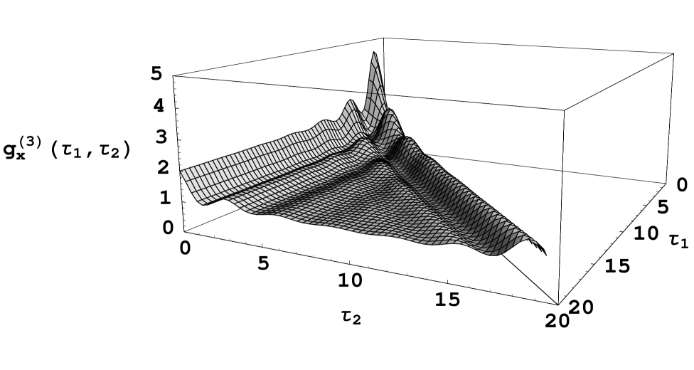
FIG. 1.: Normalized correlation function $g^{(3)}_{x}(\tau_{1},\tau_{2})$ as a function of $\tau_{1}=t_{3}-t_{1}$ and $\tau_{2}=t_{2}-t_{1}$ for $\kappa_{1}=0.15$, $\kappa_{2}=0.25$, $\bar{n}_{1}=0.01$ and $\bar{n}_{2}=0.1$, in units of the coupling constant $g$.

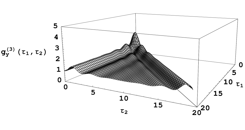
FIG. 2.: Same as Fig. 1, for $g^{(3)}_{y}(\tau_{1},\tau_{2})$.

REFERENCES

• [1] M. H. Anderson, J. R. Ensher, M. R. Mathews, C. E. Wieman, and E. A. Cornell, Science 269, 198 1995.
• [2] K. B. Davis, M. -O. Mewes, M. R. Andrews, N. J. van Drutem, D. S. Durfee, D. M. Kurn, and W. Ketterle, Phys. Rev. Lett. 75, 3969 (1995).
• [3] J. R. Ensher, D. S. Jin, M. R. Mathews, C. E. Wieman, and E. A. Cornell, Phyis. Rev. Lett. 77, 4984 (1996).
• [4] M. -O. Mewes, M. R. Andrews, N. J. van Drutem, D. S. Durfee, D. M. Kurn, and W. Ketterle, Phys. Rev. Lett. 77, 416 (1996).
• [5] C. C. Bradley, C. A. Sackett, and R. G. Hulet, Phys. Rev. Lett. 78, 985 (1997).
• [6] L. Deng et al., Nature (London) 398, 218 (1999).
• [7] S. Burger et al, cond-mat/9910487, to be published in Phys. Rev. Lett.
• [8] W. D. Phillips, S. L. Rolston et al, unpublished (1999).
• [9] M. O. Mewes et al, Phys. Rev. Lett. 78, 582 (1997).
• [10] B. P. Anderson and M. A. Kasevich, Science 282, 1686 (1998).
• [11] E. W. Hagley et al., Science 283,1706 (1999).
• [12] I. Bloch, T. W. Hänsch, T. Esslinger, Phys. Rev. Lett. 82, 3008 (1999).
• [13] S. Inouye et al. Science 285, 571 (1999).
• [14] G. A. Prataviera, E. V. Goldstein, and P. Meystre, Phys. Rev. A 60, 4846 (1999).
• [15] D. F. Walls and G. J. Milburn, Quantum Optics (Springer-Verlag, Berlin, 1994).
• [16] P. Bouyer and M. A. Kasevich, Phys. Rev. A 56, R1083 (1997).
• [17] S. Inouye et al, preprint (1999).
• [18] E. V. Goldstein and P. Meystre, Phys. Rev. Lett. 80, 5036 (1998).
• [19] R. J. Glauber, in Quantum Optics and Electronics, edited C. de Witt, A. Blandin, and C. Cohen-Tannoudji (Gordon and Breach, New York, 1965).
• [20] J. E. Thomas and L. J. Wang, Phys. Rev. A 49, 558 (1994).
• [21] C. Cohen-Tannoudji, J. Dupont-Roc, and G. Grynberg, Atom-Photon Interactions, Wiley-Interscience (New York, 1992).
• [22] M. G. Moore and P. Meystre, Phys. Rev. A 59, R1754 (1999).
• [23] M. G. Moore, O. Zobay, and P. Meystre, Phys. Rev. A 60, 1491 (1999).
• [24] P. Meystre and M. Sargent III; Elements of Quantum Optics, 3rd Edition (Springer-Verlag, Heidelberg, 1998).
——————————————————————–
Refer to caption