Born-Oppenheimer Approximation near Level Crossing

Abstract

We consider the Born-Oppenheimer problem near conical intersection in two dimensions. For energies close to the crossing energy we describe the wave function near an isotropic crossing and show that it is related to generalized hypergeometric functions ${}_{0}F_{3}$. This function is to a conical intersection what the Airy function is to a classical turning point. As an application we calculate the anomalous Zeeman shift of vibrational levels near a crossing.

Introduction. The Born-Oppenheimer (BO) problem [1] is concerned with the analysis of Schrödinger type operators where the small electron to nucleon mass ratio, plays the role of the semiclassical parameter. [2, 3, 4, 5, 6, 7, 8, 9]. The theory identifies distinct energy scales: The electronic scale which, in atomic units, is of order one and the scale of nuclear vibrations which is of order $(1/M)^{1/2}$ in these units. $M$ is the nucleus to electron mass ratio. The identification of the electrons as the fast degrees of freedom is central to the theory.

The clean splitting between fast and slow degrees of freedom fails near eigenvalue crossing of the electronic Hamiltonian where there is strong mixing between electronic and vibrational modes. This lies at the boundary of the conventional BO theory. Since the coupling between different electronic energy surfaces becomes infinite near a crossing, the nuclear wave function does not reduce to a solution of a scalar (second order) Schrödinger equation. We describe the (double surface) nuclear wave function near an isotropic conical crossing, for energies close to the energy of the crossing.

The strong mixing of the electronic and nuclear degrees of freedom near crossing leads an anomalous Zeeman effect. To describe the anomaly recall that the Zeeman splitting in molecules is reduced compared to the Zeeman splitting of atoms. It is convenient to parameterize the reduction by a parameter $\gamma$ so that the Zeeman splitting is of the form (and order) $M^{-\gamma}B$ with $B$ the external magnetic field. The low lying vibrational levels have large reduction, $\gamma=1$. This is what one expects from nuclei whose magnetic moments are by factor $M$ smaller than the Bohr magneton. Levels near the crossing energy can have a small reduction expressed by the fact that $\gamma<1$. For the isotropic situation we calculate $\gamma=1/6$, so that the Zeeman shift is anomalously large, by a factor of about 2000, than the normal Zeeman splitting of molecular levels. More precisely, we find that the Zeeman splitting near isotropic crossing is

$$\Delta E(m)\approx\frac{1}{M^{1/6}}\frac{g(m)}{T_{e}}\,B.$$ (1)

The sign $\approx$ means equality in the limit $M\to\infty$. $B$ is proportional to the magnetic field, with a coefficient dependent only on the electronic wave functions at the crossing. $m$, a half odd integer, is the azimuthal quantum number, $T_{e}$ is an electronic time scale, see Eq. (21) below. $g(m)$ is a universal dimensionless factor which is determined by the nuclear wave function near the crossing, see Eq. (20) below. As we shall see $g(m)=-g(-m)$ and numerical estimates of Eq. (20) give

$$g\left(\frac{1}{2}\right)=0.961,\,\,g\left(\frac{3}{2}\right)=0.543,\,\,g\left(\frac{5}{2}\right)=0.396.$$ (2)

$g(m)$ is a molecular analog of the Landé g factor in atoms: So, while Langé g factor describes the Zeeman shift due to the mixing of spin and orbital degrees of freedom, $g(m)$ does it for the nuclear and electronic ones.

One can formulate the BO problem in the following way [5]:

$$H_{bo}=-\frac{1}{M}\Delta_{x}+H_{e}(x),$$ (3)

where $H_{e}(x)$, the electronic Hamiltonian, depends parameterically on the nuclear coordinates $x$. When time reversal is not broken, $H_{e}(x)$ is a real symmetric matrix [10]. The Wigner von Neumann crossing rule [11] says that $H_{e}(x)$ has generically a crossing point for two modes of vibrations, $x\in{\rm I\kern-1.99997ptR}^{2}$.

Here we shall consider the simple scenario where $H_{e}(x)$ is a $2\times 2$ matrix of and $x\in{\rm I\kern-1.99997ptR}^{2}$. This means that we shall treat only the restriction of the electronic Hamiltonian to the two dimensional subspace spanned by the two degenerate eigenstates at the crossing point. We shall assume that $H_{e}(x)$ has a single crossing point at $x=0$, and set the crossing energy at $0$. We further assume that the crossing is conic, that $H_{e}(x)$ is isotropic about the origin, and that the $x$ dependence of $H_{e}(x)$ is smooth near the origin. This is a common model [7].

We first recall why the standard BO theory fails near a crossing. When $H_{e}(x)$ is symmetric it can be diagonalized by an orthogonal transformation $R(x)$. In the $2\times 2$ case, and when $H_{e}(x)$ is non-degenerate, $R(x)$ is uniquely determined, up to an overall sign, by requiring $\det R(x)=1$. Hence, away from crossing, $H_{bo}$ is unitarily equivalent to

$$-\frac{1}{M}\Big{(}\nabla_{x}+iA(x)\Big{)}^{2}+\pmatrix{E_{1}(x)&0\cr 0&E_{2}(x)},$$ (4)

where $E_{1,2}(x)$ are the two eigenvalues of $H_{e}(x)$. The vector potential $A(x)=-iR^{T}(x)\nabla_{x}R(x)$ is purely off-diagonal. For linear crossing, $R(x)\to-R(x)$ as $x$ surrounds the origin [4]. This forces a $1/|x|$ singularity of the vector potential for small $x$. Far from the origin, to leading order in $1/M$, the two components of the wave function decouple and are given by

$$\Psi_{bo,j}(x)\approx\psi_{cl,j}(x)R(x)\pmatrix{\delta_{j,1}\cr\delta_{j,2}},\quad j=1,2,$$ (5)

where $\psi_{cl,j}$ is a semiclassical solution of the Schrödinger equation with potential $E_{j}(x)$ in the cut plane with antiperiodic boundary conditions [4, 7]. This decoupling holds provided $|x|>>M^{-1/3}$ [20]. We shall henceforth denote $\epsilon=M^{-1/3}$, and refer to the region $|x|>>\epsilon$ as ”far from the crossing”. In contrast, the divergence of the off diagonal part of $A$ near the crossing prevents such a decoupling near the crossing. Our aim is to analyze the BO theory, to leading order in $\epsilon$, near the crossing of $H_{e}$. The reason one can still hope to say something useful near the crossing is that the asymptotic form of $H_{e}(x)$ near the crossing, i.e. for $|x|<<1$, is universal [6]

$$H_{e}(x)=x_{1}\sigma_{1}+x_{2}\sigma_{3}+O(x^{2})$$ (6)

where $\sigma$ are the Pauli matrices. We shall refer to $|x|<<1$ as ”close to the crossing”. Notice that our notions of close and far from the crossing have a nonempty intersection. This enables us to match the solution close to the crossing with the standard, decoupled, BO solution, Eq. (5).

The zero energy wave function close to the crossing. We study the wave functions near the crossing for energies close to the crossing energy. Everything to be said from now on is true in the limit of $M\to\infty$, to leading order in negative powers of $M$.

We shall assume that zero is an eigenvalue of (3), since there is always an eigenvalue that is close enough to zero [20]. It turns out to be convenient first to unitary-transform (6) with $e^{-i\frac{\pi}{4}\sigma_{1}}$. This will replace $\sigma_{3}$ in (6) by $\sigma_{2}$. In this representation, close to the crossing the zero energy wave function satisfies approximately the differential equation

$$\left\{-\nabla_{\xi}^{2}+\xi_{1}\sigma_{1}+\xi_{2}\sigma_{2}\right\}\Psi(\xi_{1},\xi_{2})=0$$ (7)

$\Psi$ stands for a two component column matrix and $\xi_{i}=M^{1/3}\,x_{i}$ is a scaled variable.

The operator $J_{3}=L_{3}+\frac{1}{2}\sigma_{3}=-i\xi_{1}\partial_{\xi_{2}}+i\xi_{2}\partial_{\xi_{1}}+\frac{1}{2}\sigma_{3}$ commutes with the operator on the l.h.s. of (7). It does not have the meaning of total angular momentum, since the Pauli matrices do not represent spin. We thus consider solutions of the differential equation (7) which are eigenfunctions of $J_{3}$ with an eigenvalue $m$, namely:

$$\Psi(\xi;m)=e^{im\theta}\,\pmatrix{\varphi_{1}(\rho;m)e^{-i\theta/2}\cr\varphi_{2}(\rho;m)e^{i\theta/2}}$$ (8)

$\rho,\theta$ are the polar coordinates related to $\xi$. $m$ must be half odd integer, for the wave function to be single valued. Separating variables, the radial equation obtained from (7), in the $m$-th sector, takes the form:

$$\left\{-\frac{d^{2}}{d\rho^{2}}-\frac{1}{\rho}\frac{d}{d\rho}+\frac{m^{2}+\frac{1}{4}}{\rho^{2}}+\pmatrix{-\frac{m}{\rho^{2}}&\rho\cr\rho&\frac{m}{\rho^{2}}}\right\}\pmatrix{\varphi_{1}\cr\varphi_{2}}=0$$ (9)

Of the four linearly independent solutions of Eq. (9), basically due to boundary conditions, only one linear combination is fit to represent a wave function. We denote it by ${\cal F}_{c}(m,\rho)$ and its components by $\varphi_{1c}(m;\rho)$ and $\varphi_{2c}(m;\rho)$. ${\cal F}_{c}(m,\rho)$ is to a crossing point what the Airy function is to a classical turning point [12, 13]: It interpolates between the near region where the wave function is intrinsically a two component spinor, and the far region where the wave function is highly oscillatory and given by Eq. (5). ${\cal F}_{c}(m,\rho)$ has a closed expression in terms of the generalized hypergeometric functions of the kind ${}_{0}F_{3}$. It has the asymptotic (for $\rho>>1$) form

$${\cal F}_{c}(m,\rho)\approx\frac{1}{\rho^{3/4}}\,\cos\left({\frac{2}{3}}\rho^{3/2}-\pi\left(\frac{m}{3}+\frac{1}{4}\right)\right)\pmatrix{1\cr-1},$$ (10)

Solving (9) asymptotically near the origin gives[15]

$$\pmatrix{\varphi_{1}(\rho;m)\cr\varphi_{2}(\rho;m)}\sim\pmatrix{a_{+}\rho^{m-1/2}+a_{-}\rho^{-m+1/2}\cr b_{+}\rho^{m+1/2}+b_{-}\rho^{-m-1/2}}$$ (11)

Solving (9) asymptotically at infinity we obtain

$$\pmatrix{\varphi_{1}(\rho;m)\cr\varphi_{2}(\rho;m)}\sim\frac{1}{\rho^{3/4}}\left\{\left(A_{+}e^{z}+A_{-}e^{-z}\right)\pmatrix{1\cr 1}+C\cos\left(z+\phi\right)\pmatrix{1\cr-1}\right\},\quad z={\frac{2}{3}}\rho^{3/2}$$ (12)

The four dimensional family of solutions can be parameterized by either $a_{+},a_{-},b_{+},b_{-}$ or $A_{+},A_{-},C,\phi$. Requiring the solution to be bounded at the origin and at infinity means (for positive $m$) that $A_{+}=0,a_{-}=0,b_{-}=0$. Imposing three homogeneous conditions on a four dimensional linear space leaves us with one dimensional subspace, i. e. a certain function times an arbitrary constant. This is the celebrated ${\cal F}_{c}(\rho,m)$.

While the reason we require ${\cal F}_{c}(\rho,m)$ to be bounded at the origin is obvious, the reason we require it to be bounded at infinity is a bit subtle, since (9) is meaningful only close to the crossing. However, ”close to the crossing”, $\rho<<M^{1/3}$, extends farther and farther in terms of $\rho$ as $M$ gets large. $A_{+}$ at (12) should be exponentially small, and can set to zero to leading order.

The solutions which are regular at the origin can be obtained from the fourth order differential equations, one for each component $\varphi_{j}$, obtained from (9). These are related to the differential equation that defines the generalized hypergeometric functions ${}_{0}F_{3}$. The two linearly independent solutions that are regular at the origin are [20]:

$${\cal F}_{1}(\rho;m) = \pmatrix{\rho^{m-\frac{1}{2}}{{}_{0}F_{3}}(;\frac{1}{3},\frac{1}{2}+\frac{m}{3},\frac{5}{6}+\frac{m}{3};\frac{\rho^{6}}{6^{4}})\cr\frac{\rho^{m+\frac{5}{2}}}{6+4m}{{}_{0}F_{3}}(;\frac{4}{3},\frac{3}{2}+\frac{m}{3},\frac{5}{6}+\frac{m}{3};\frac{\rho^{6}}{6^{4}})};$$ (13)

$${\cal F}_{2}(\rho;m) = \pmatrix{\frac{\rho^{m+\frac{7}{2}}}{12+8m}{{}_{0}F_{3}}(;\frac{5}{3},\frac{3}{2}+\frac{m}{3},\frac{7}{6}+\frac{m}{3};\frac{\rho^{6}}{6^{4}})\cr\rho^{m+\frac{1}{2}}{{}_{0}F_{3}}(;\frac{2}{3},\frac{1}{2}+\frac{m}{3},\frac{7}{6}+\frac{m}{3};\frac{\rho^{6}}{6^{4}})},$$ (15)

where ${}_{0}F_{3}(;a,b,c;\rho)$ are generalized hypergeometric functions [16, 17]. The linear combination

$${\cal F}_{c}(\rho;m)=A_{1}(m){\cal F}_{1}(\rho;m)+A_{2}(m){\cal F}_{2}(\rho;m)$$ (16)

is bounded at infinity provided [20]:

$$A_{j}(m)=\frac{-(-1)^{j}2\pi^{3/2}6^{\frac{(-1)^{j}-2m}{3}}}{3\Gamma(\frac{1}{2}+\frac{m}{3})\Gamma(\frac{1}{2}-\frac{(-1)^{j}}{6})\Gamma(1+\frac{2m-(-1)^{j}}{6})}$$ (17)

We have set the global coefficient in front of (16) such that (10) will be true. Formulae (13-17) are correct only for positive $m$-s. Their negative counterparts can be obtained by interchanging the lower and upper components, as can be seen from (9).

The anomalous Zeeman shift. Let us now turn to the Zeeman shift. The magnetic field breaks time reversal symmetry, which means that it adds an the imaginary term to $H_{e}(x)$, in the representation where $H_{e}(x)$ is real. Generically the magnetic field will remove the conical intersection of $H_{e}(x)$ at $x=0$ and create a gap between the two energy sheets. The gap will be proportional to the magnetic field in atomic units, and the coefficient will be in general of order one. We can therefore introduce the magnetic field into our model by adding the term $B\sigma_{2}$ to $H_{e}(x)$ at (6). There is no harm in taking $B$ to be independent of $x$, since only the value of $B$ in the origin will be of importance to us. $B$ is therefore a constant, proportional to the magnetic field in atomic units. We shall not minimally couple the magnetic field directly to the vibrations for this turns out to be a weaker effect, of order $M^{-1}$, while the shift mediated by the electrons, in the rotationally invariant case, is $M^{-1/6}$, as we shall see.

Let us consider the case where the rest of $H_{e}(x)$, namely the $O(x^{2})$ part in (6), does not break the full rotational symmetry of its linear part, so that $m$ is still a good quantum number.

In the rotational invariant case, the model has, for $B=0$, a two-fold degeneracy: The states $m$ and $-m$ are degenerate. The magnetic field $B$ breaks this degeneracy. The splitting is twice the Zeeman shift in the energy for the two states $\pm m$ move in opposite directions.

Equipped with approximants to the wave function near and far from the crossing, with a degenerate perturbation theory one can calculate, to leading order in $1/M$, the Zeeman splitting and obtain (1). We describe this calculation in details elsewhere [20]. Here we would only like to sketch the derivation of the power in (1).

Far from the crossing, one can neglect the vector potential in (4). The WKB approximant to the radial part of $\psi_{cl,2}$ is

$$\psi_{cl,2}(r)\approx\frac{N}{r^{3/4}}\cos(\sqrt{M}\frac{2}{3}r^{3/2}+\phi),$$ (18)

where we have employed the linearity of the energy surfaces near the crossing. It is a general property of the WKB approximation, that the normalization coefficient $N$ is independent of $M$, to leading order in $1/M$. From (10) and (18) one sees that the interpolation of the BO radial wave function towards the crossing is

$$\Psi(r;m)\approx NM^{1/4}{\cal F}_{c}(m;M^{1/3}r).$$ (19)

$B$ removes the degeneracy of the electronic levels at $x=0$. The gap created there due to $B$ is equal to $2B$. Intuitively, the Zeeman shift of a vibrational level will be proportional to the amount of probability density in the vicinity of the crossing times $B$. By “vicinity” we mean a neighbourhood of order $M^{-1/3}$ of the origin, the area of which is of order $M^{-2/3}$. The density associated with the wave function is large there and by (19) is proportional to $M^{1/2}$. Hence the weight is proportional to $(M)^{-1/6}$ which gives the power of the Zeeman splitting in Eq. (1). The coefficient of proportion will include an integral over the components of $\cal F$, [20], which gives $g(m)$

$$g(m)=\int_{0}^{\infty}\rho\,d\rho\,(\varphi_{1c}^{2}(\rho;m)-\varphi_{2c}^{2}(\rho;m)).$$ (20)

N gives the factor $1/T_{e}$, where $T_{e}$ is

$$T_{e}=\int dr\frac{1}{\sqrt{-E_{1}(r)}},$$ (21)

The integration is carried out between the two turning points of $E_{1}$, the negative energy sheet (4). Eq. (21) is proportional to the time in takes a particle with a unit (electronic) mass to travel classically across the potential. It is independent of the nuclear mass, and $T_{e}^{-1}$ has the order of magnitude of electronic energies. From the invariance under $T$ of $H_{bo}(B=0)$ it follows that $g(m)=-g(-m)$.

One motivation for this work was an attempt to gain some understanding of the different status of crossing in theory and experiment. Theory puts crossing and avoided crossing in distinct baskets: conic crossings come with fractional azimuthal quantum numbers while avoided crossings come with integral quantum numbers. In contrast, measurements of molecular spectra normally can not tell a crossing from near avoided crossing. Only with precision measurements [18] and precise quantum mechanical calculations [19] can one tell when molecular spectra favor an interpretation in terms of crossing and half integral quantum numbers or avoided crossing with integral quantum numbers. Zeeman splitting appears to be a useful tool to study crossing. The anomaly of crossing is characterized by a fractional power $\gamma$ of the molecular reduction of the Zeeman splitting, $M^{-\gamma}$. A system of choice for studying crossing is molecular trimers [18, 19]. Since trimers are not rotationally invariant Eq. (1) does not apply and we can not conclude that near crossing $\gamma=1/6$ for trimers. However, it is natural to expect that the qualitative features of our results carry over also to the non-isotropic case where crossing will manifest itself by an anomalously large Zeeman splitting and a fractional $\gamma$. It is an interesting challenge to calculate or measure the value of $\gamma$ for (other) molecular crossings, and trimers in particular.

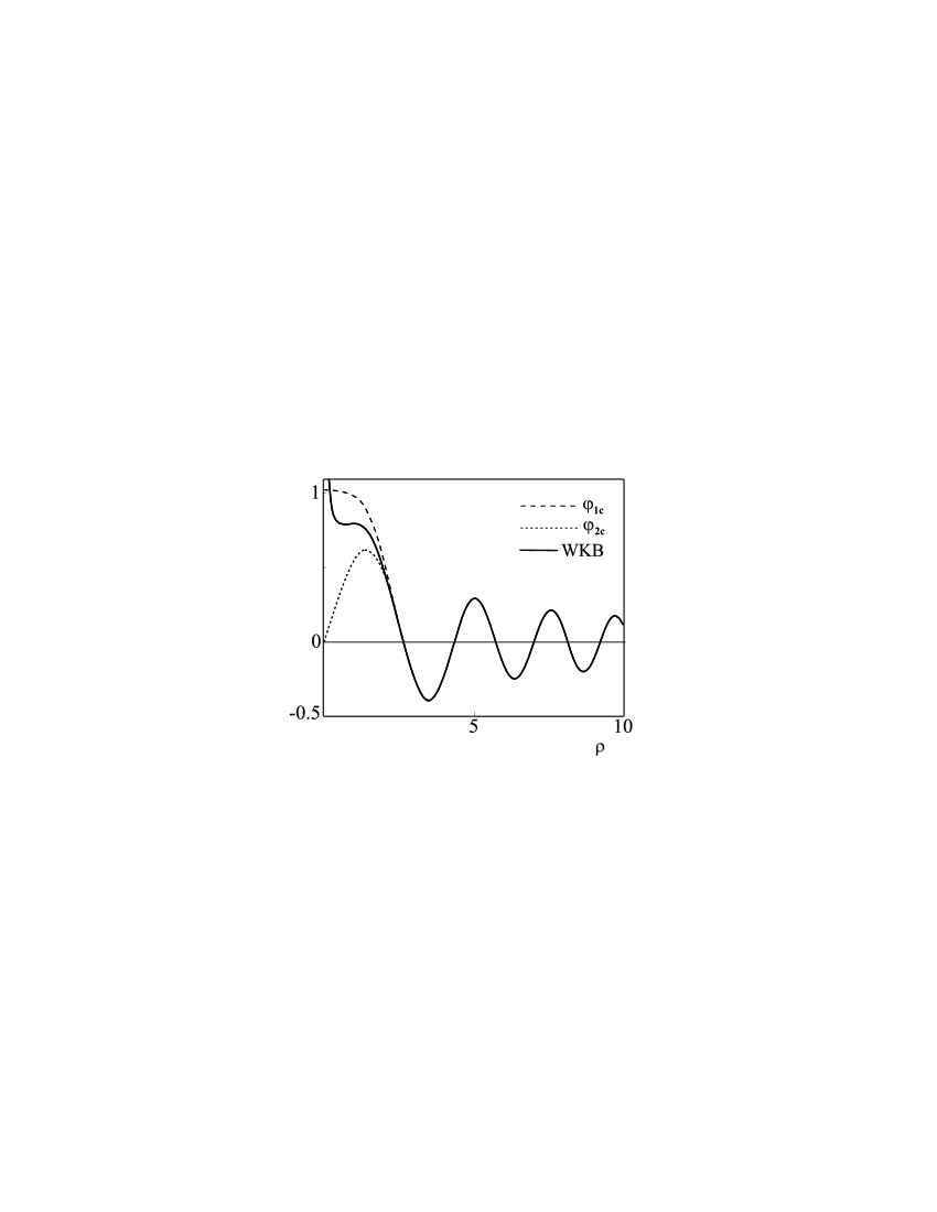
FIG. 1.: The components of ${\cal F}_{c}(m;\rho)$ for $m=\frac{1}{2}$ and their asymptotic form given by (10), which is also the BO wave function approximated by WKB.

REFERENCES

- [1] M. Born and R. Oppenheimer, Ann. Phys. (Leipzig) 84, 457 (1927)
- [2] P. Aventini and R. Seiler, Comm. Math. Phys, 41, 2, 34 (1975); F. Bornemann, Homogenization in time of singularly perturbed mechanical systems, Lecture notes in Mathematics 1687, Springer (1998); J.M. Combes, P. Duclos and R. Seiler, in Rigorous atomic and molecular physics, G. Velo and A. Wightman Ed., Plenum (1981) G.A. Hagedorn, Ann. Inst. H. Poincaré 47,1-16,(1987); M. Klein, A. Martinez, R. Seiler and X.P. Wang, Comm. Math. Phys. 144, 607-639 (1992)
- [3] M.V. Berry, Proc. R. Lond. A392 45 (1984)
- [4] H. C. Longuet-Higgins, U. Öpik, M. H. L. Pryce, and R. A. Sack, Proc. Roy. Soc. London, Ser. A 244, 1 (1958).
- [5] C. A. Mead, Rev. Mod. Phys. 64, 51, (1992)
- [6] C. A. Mead, J. Chem. Phys. 78, 807 (1983); T.C. Thompson, D.G. Trulhar and C.A. Mead, J. Chem. Phys. 82, 2392 (1985);T.C. Thompson and C.A. Mead, J. Chem. Phys. 82, 2409 (1985).
- [7] C. A. Mead and D. G. Truhlar, J. Chem. Phys. 70, 2284 (1979)
- [8] R. Jackiw, Int. J. Mod. Phys. A3 (1988)
- [9] A. Shapere and F. Wilczek, Geometric Phases in Physics, World Sceintific, Singapore (1989).
- [10] Strictly, on should distinguish the case of an integral spin from the case of half-integrla spin where is quaternionic real see F. Dyson, J. Math. Phys. 3 140, (1964)
- [11] J. von Neumann and E. P. Wigner, Phys. Z. 30 (1929), 467,
- [12] L. D. Landau and E. M. Lifshitz, Quantum Mechnics Perganom Press, 3-rd ed. (1977).
- [13] J. L. Powell and B. Crasemann, Quantum Mechanics, Addison-Wesley (1961).
- [14] E. P. Wigner, Group Theory and its Application to the Quantum Mechanics of Atomic Spectra, N. Y. Academic Press (1959).
- [15] This is strictly true for , the case requires a special treatment see e.g. W. E. Boyce and R. C. Diprima, Elementary Differential Equations, Wiley, 6-th ed. (1997).
- [16] H. Bateman, Higher Transcendental Functions, McGraw-Hill (1953)
- [17] S. Iyanaga and Y. Kawada, Encyclopedic Dictionary of Mathematics, MIT Press (1968).
- [18] H. von Busch, Vas Dev, H.A. Eckel, S Kasahara, J. Wang, W. Demtöder, P. Sebald and W. Meyer, Phys. Rev. Lett. 81, 4584, (1998)
- [19] B. Kendrick, Phys. Rev. Let. 79, 13, 2341 (1997).
- [20] A. Gordon and J.E. Avron, in preparation