How Events Come Into Being: EEQT, Particle Tracks, Quantum Chaos, and Tunneling Time

Abstract

In sections 1 and 2 we review Event Enhanced Quantum Theory (EEQT). In section 3 we discuss applications of EEQT to tunneling time, and compare its quantitative predictions with other approaches, in particular with Büttiker-Larmor and Bohm trajectory approach. In section 4 we discuss quantum chaos and quantum fractals resulting from simultaneous continuous monitoring of several non-commuting observables. In particular we show self-similar, non-linear, iterated function system-type, patterns arising from quantum jumps and from the associated Markov operator. Concluding remarks pointing to possible future development of EEQT are given in section 5.

1 Introduction

Event-Enhanced Quantum Theory (EEQT) was developed in response to John Bell’s concerns about the status of the measurement problem in quantum theory [1, 2]. The main thrust of quantum measurement theory is to explain the mechanism by which potential properties of quantum systems become actual. At the present time, this is no longer an abstract or philosophical problem since it is now possible to carry out prolonged observations of individual quantum systems. These experiments provide us with time series data, and a complete theory must be able to explain the mechanism by which these time series are being generated; moreover it must be in position to “simulate” the process of events generation.

John Bell sought a solution to the measurement problem in hidden variable theories of Bohm and Vigier, his own idea of beables, and also in the spontaneous localization idea of Ghirardi, Rimini and Weber [3]. More recently we have proposed a formalism going in a similar direction, but avoiding the introduction of hidden variables beyond the wave function itself [4, 5, 6].

EEQT offers a mathematically consistent way of coupling between a quantum and a classical system. The classical system $C$ is described by an Abelian algebra ${\cal A}_{c}$. In this respect, EEQT is indeed an enhancement because it modifies the quantum dynamics by adding a new term to the Liouville equation. This allows unification of the continuous evolution of quantum states with quantum jumps that accompany real world events. When the coupling $Q-C$ is weak, events are sparse and EEQT reduces to the standard quantum theory.

In this EEQT framework, a measurement process is a coupling $Q-C$, where transfer of information about the quantum state to the classical recording device is mathematically modeled by a semigroup of completely positive and trace-preserving maps of the total system $Q\times C$. Let us emphasize that such a transfer of information cannot, indeed, be implemented by a Hamiltonian or more generally by any automorphic evolution [7, 8].

To illustrate this last point, let us consider the total system $Q\times C$ described by an algebra of operators ${\cal A}$ with center $z={\cal A}_{c}$. The center describes the classical degrees of freedom. Let $\omega$ be a state of ${\cal A}$ and let $\omega_{c}$ denote its restriction to ${\cal A}_{c}$. Let $\alpha_{t}$ be an automorphic time evolution of ${\cal A}$ and $\omega_{t}=\alpha_{t}(\omega)$ the dual evolution of states given by $\alpha^{t}_{t}(\omega)(A)=\omega(\alpha_{t}(A))$. Each automorphism of $\cal A$ leaves its center invariant, which implies that $\alpha_{t}(\omega)_{c}=\alpha^{t}|_{z}(\omega_{c})$. In other words $\omega^{t}_{c}$ depends only on $\omega^{0}_{c}$ and the state at time $t$ of $C$ depends only on the part of $C$ and not on its extension to the total system $Q\times C$. The result is that to have information transfer from the total system to its classical subsystem we must use non automorphic time evolutions.

The formal development of EEQT was inspired by the works of Jauch [9], Hepp [10], Piron [11, 12, 13], Gisin [14, 15], Araki [16] and Primas [17, 18]. In [19, 20] M.H.A. Davis described a special class of piecewise deterministic Markov processes that reproduced the master equation postulated in [4]. This opened a new chapter of EEQT and allowed for description of individual quantum systems. In [21] it was proven that the class of couplings considered in EEQT leads to a unique piecewise deterministic Markov process taking values on the pure state space of the total system $Q\times C$. This process consists of random jumps accompanied by changes of the classical state, interspersed by random periods of Schrödinger like deterministic evolution. The process is nonlinear in the quantum pure state $\psi$ and after averaging we recover the original linear master equation for statistical states of the total system $Q\times C$.

The crucial concept of EEQT is that of a classical, discrete and irreversible event. This is taken into account by including, from the beginning, classical degrees of freedom. Once the existence of the classical part is accepted then “events” can be defined as changes of pure state of this classical part $C$. In EEQT events do happen and they do it in finite time. Rudolf Haag [22] takes a similar position and calls it an “evolutionary picture”. According to this view the future does not yet exist and is being continuously created, this creation being marked by events.

In EEQT we have a flow of information from $Q$ to $C$ and moreover a way to calculate numbers in real experiments and to model the feedback from $C$ to $Q$. The coupling $Q\times C$ does not mean we are taking a step backward into classical mechanics. We are only claiming that not all is quantum and that there are elements of Nature that are not, and cannot be, described by a quantum wave function. This assumption is confirmed everyday by experiments which clearly show that we are living in a world of facts and not in a world of potentialities. For this aspect which is not reducible to quantum degrees of freedom we use the term ”classical variables”. This does not imply that we impose any restriction on their nature.

At this point we would like to emphasize a fundamental difference between the classical variables of EEQT and the additional parameters introduced in hidden variable theories. Hidden variable theories consider microscopic variables that are hidden from our observation. EEQT deals with classical variables that can be directly observed. They are a direct counterpart of Physics on the other side of the Heisenberg-von Neumann cut. Another important point is that in hidden variable theories there is no back action of these variables on the wave function. In EEQT we have a feedback of $C$ on $Q$. EEQT can be also considered as a final result of a decoherence mechanism as described in [23, 24]. In section 2 the mathematical formalism of EEQT is presented. In sections 3 and 4 some applications are described. Concluding remarks are given in section 5.

2 EEQT – The mathematical formalism

We will only describe the case of a discrete classical system $C$. It has been shown in [25], while applying EEQT to SQUID, how to extend the formalism in cases where the classical system $C$ is continuous. There are two levels in EEQT - the ensemble level and the individual level. This is in a total contradistinction to the standard quantum theory which deals only with ensembles and even claims, rather often, that individual description is impossible! Let us begin with the ensemble level.
First of all, in EEQT, at that level, we use all the standard mathematical formalism of quantum theory, but we extend it adding an extra, possibly multidimensional, parameter $\alpha.$ Thus all quantum operators $A$ get an extra index $A_{\alpha}$, quantum Hilbert space ${\cal H}$ is replaced by a family ${\cal H}_{\alpha},$ quantum state vectors $\psi$ are replaced by families $\psi_{\alpha},$ quantum Hamiltonian $H$ is replaced by a family $H_{\alpha}$ etc.
The parameter $\alpha$ is used to distinguish between macroscopically different and non-superposable states of the universe. In the simplest possible model we are interested only in describing a ”yes-no” experiment and we disregard any other parameter - in such a case $\alpha$ will have only two values $0$ and $1$. Thus, in this case, we will need two Hilbert spaces. This will be the case when we will deal with sharp particle detectors. In a more realistic situation $\alpha$ will take values in a multi-dimensional, perhaps even infinite-dimensional manifold. But even that may prove to be insufficient.

When, for instance, EEQT is used as an engine powering Everett-Wheeler many-world branching-tree, in such a case, $\alpha$ will also have to have the corresponding dynamical branching-tree structure, where the space in which the parameter $\alpha$ takes values, grows and becomes more and more complex together with the growing complexity of the branching structure.

An “event” is, in our mathematical model, represented by a change of $\alpha$, $\alpha$ representing a pure state of the classical subsystem $C$. This change is discontinuous, is a branching. Depending on the situation this branching is accompanied by a more or less radical change of physical parameters. Sometimes, such as in the case of a phase transition in Bose-Einstein condensate, we will need to change the nature of the underlying Hilbert space representation. In other cases, such as the case of a particle detector, the Hilbert spaces ${\cal H}_{0}$ and ${\cal H}_{1}$ will be indistinguishable copies of one standard quantum Hilbert space ${\cal H}.$

Another important point is this: time evolution of an individual quantum system is described by piecewise continuous function $t\mapsto\alpha(t)$, $\psi(t)\in{\cal H}_{\alpha}(t)$, a trajectory of a piecewise deterministic Markov process (in short: PDP), where periods of continuous evolution are interspersed by discontinuous catastrophic jumps.

As already pointed out above, in EEQT any non-trivial coupling of classical to quantum degrees of freedom involves back-action of classical on quantum. This back-action shows up in a dual way: in changes to the continuous evolution (as in ”interaction free measurements”) and also in discontinuous jumps and branchings. It is impossible to understand the essence of this back-action without having even a rough idea about PDPs.

Originally EEQT was described in terms of a master equation for a coupled, quantum+classical, system; thus it was only applicable to ensembles; the question of how to describe individual systems was open. Then, after searching through the mathematical literature, we found that, in his monographs [19, 20] dealing with stochastic control and optimization, M. H. A. Davis described a special class of piecewise deterministic processes that fitted perfectly the needs of quantum measurement theory, and that reproduced the master equation postulated originally by us in Ref. [4]. The special class of couplings between a classical and quantum system leads to a unique piecewise deterministic process with values on $E$-the pure state space of the total system. This process consists of random jumps, accompanied by changes of a classical state, interspersed by random periods of Schrödinger-type (but non-unitary) deterministic evolution. The process, although mildly nonlinear in quantum wave function $\psi$, after averaging, recovers the original linear master equation for statistical states.

We would like to stress that, in EEQT, the dynamics of the coupled total system which is being modeled is described not only by a Hamiltonian ${\cal H}$, or better: not only by an $\alpha$– parametrized family of Hamiltonians $H_{\alpha}$, but also by a doubly parametrized family of operators $\{g_{\beta\alpha}\}$, where $g_{\beta\alpha}$ is a linear operator from ${\cal H}_{\alpha}$ to ${\cal H}_{\beta}$. While Hamiltonians must be essentially self-adjoint, $g_{\beta\alpha}$ need not be such – although in many cases, when information transfer and control is our concern (as in quantum computers), one wants them to be even positive operators (otherwise unnecessary entropy is created).

It should be noted that the time evolution of statistical ensembles is, due to the presence of $\{g_{\beta\alpha}\}$’s, non-unitary or, using algebraic language, non-automorphic. The system, as a whole, is open. This is necessary, as we like to emphasize: information (in this case: information gained by the classical part) must be paid for with dissipation! There is no free lunch!

A general form of the linear master equation describing statistical evolution of the coupled system is given by

$${\dot{A}}_{\alpha}=i[H_{\alpha},A_{\alpha}]+\sum_{\beta}g_{\beta\alpha}^{\star}A_{\beta}g_{\beta\alpha}-{1\over 2}\{\Lambda_{\alpha},A_{\alpha}\},$$ (1)

$${\dot{\rho}}_{\alpha}=-i[H_{\alpha},\rho_{\alpha}]+\sum_{\beta}g_{\alpha\beta}\rho_{\beta}g_{\alpha\beta}^{\star}-{1\over 2}\{\Lambda_{\alpha},\rho_{\alpha}\},$$ (2)

where

$$\Lambda_{\alpha}=\sum_{\beta}g_{\beta\alpha}^{\star}g_{\beta\alpha}.$$ (3)

The operators $g_{\alpha\beta}$ can be allowed to depend explicitly on time. While the term with the Hamiltonian describes ”dyna-mics”, that is exchange of forces, of the system, the term with $g_{\alpha\beta}$ describes its ”bina-mics” - that is exchange of ”bits of information” between the quantum and the classical subsystem.

As has been proven in [21] the above Liouville equation, provided the diagonal terms $g_{\alpha\alpha}$ vanish, can be considered as an average of a unique Markov process governing the behavior of an individual system. The real–time behavior of such an individual system is given by a PDP process realized by the following non–unitary, non–linear and non–local, EEQT algorithm:

PDP Algorithm Suppose that at time $t_{0}$ the system is described by a quantum state vector $\psi_{0}$ and a classical state $\alpha$. Then choose a uniform random number $p\in[0,1]$, and proceed with the continuous time evolution by solving the modified Schrödinger equation

$${\dot{\psi}_{t}}=(-iH_{\alpha}dt-{1\over 2}\Lambda_{\alpha})\psi_{t}$$

with the initial wave function $\psi_{0}$ until $t=t_{1}$, where $t_{1}$ is determined by

$$\int_{t_{0}}^{t_{1}}(\psi_{t},\Lambda_{\alpha}\psi_{t})dt=p.$$

Then jump. When jumping, change $\alpha\rightarrow\beta$ with probability

$$p_{\alpha\rightarrow\beta}=\|g_{\beta\alpha}\psi_{t_{1}}\|^{2}/(\psi_{t_{1}}\Lambda_{\alpha},\psi_{t_{1}}),$$

and change

$$\psi_{t_{1}}\rightarrow\psi_{1}=g_{\beta\alpha}\psi_{t_{1}}/\|g_{\beta\alpha}\psi_{t_{1}}\|.$$

Repeat the steps replacing $t_{0},\psi_{0},\alpha$ with $t_{1},\psi_{1},\beta$.

The algorithm is non–linear, because it involves repeated normalizations. It is non-unitary because of the extra term $-{1\over 2}\Lambda_{\alpha}$ in the exponent of the continuous evolution. It is non–local because it needs repeated computing of the norms - they involve instantaneous space–integrations. It is to be noted that PDP processes are more general than the popular diffusion processes. In fact, every diffusion process can be obtained as a limit of a family of PDP processes.

3 Cloud chamber model, GRW Spontaneous Localization Theory and Born’s Interpretation

In this example, we wish to account for the tracks that quantum particles leave in cloud chambers. Physically a cloud chamber is a highly complex system. To describe the response of the chamber to a quantum particle it is sufficient to assume that we have to deal with a collection of two state systems able to change their state when a particle passes near a sensitive center. Let us sketch the model proposed in [26, 27].

Let us consider the space $E={\bf R}^{3}$ as filled with a continuous medium (photographic emulsion, super-saturated vapor, etc.) which can be at each point $a\in E$ in one of two states: “on” represented by ${1\choose 0}$ and “off” represented by ${0\choose 1}$. The set of all possible states of the system is then $2^{E}$. But we are only interested with a continuum of states - namely the “vacuum” (i.e. when all points of the medium are in “off” state)- and states which differ from the vacuum only in a finite number of points. We define ”event” to be a change of state of a finite number of points. Thus the space of classical events can be identified with the space of finite subsets of $E$ from which it follows that the total system $\Sigma_{tot}=\Sigma_{q}\otimes\Sigma_{c}$ is described by families $\{\rho_{\Gamma}\}\subset E$, $\Gamma$ finite subset of $E$. For each $a\in E$ let $g_{a}$ be a Hermitian bounded operator which represents heuristically the sensitivity of the two-state detector located at $a$. We can think of $g_{a}$ as a gaussian function $g_{A}(x)$ centered at $x=a$ (other phenomenological shapes are also possible). We denote

$$\int_{E}g^{2}_{a}(x)da=\Lambda(x)\ .$$ (4)

The quantum mechanical Hilbert space is then ${\cal H}_{q}=L^{2}({\bf R}^{3},dx)$. Each state $\rho$ of the total system can be, formally, written as $\rho=\Sigma_{\Gamma\in{\cal S}}\rho_{\Gamma}\otimes\epsilon_{\Gamma}$, where, for $\Gamma\in{\cal S}$,

$$\epsilon_{\Gamma}=\prod\otimes_{a\in E}\left(\begin{array}[]{cc}\chi_{\Gamma}(a)&0\\ 0&1-\chi_{\Gamma}(a))\end{array}\right)\,$$ (5)

and where $\chi_{\Gamma}$ stands for the characteristic function of $\Gamma$. The Lindblad coupling is now chosen in the following way

$$L_{int}(\rho)\equiv\int_{{\bf R}^{3}}da\left[V_{a}\rho V_{a}-\frac{1}{2}\{V^{2}_{a},\rho\}\right]$$ (6)

where $V_{a}=g_{a}\otimes\tau_{a},\tau_{a}$ denoting the flip at the point $a\in{\bf R}^{3}$. Let us introduce the following notation: $a(\Gamma)$ represents the state $\Gamma$ with the counter at position $a$ flipped, i.e. $a(\Gamma)=(\Gamma\backslash\{a\}\cup\{\{a\}\backslash\}$. The Liouville equation is given by $\dot{\rho}=-i\left[H,\rho\right]+L_{int}(\rho)$. But using the following identity in eq. (6)

$$V_{a}\rho V_{a}=\sum_{\Gamma}g_{a}\rho_{\Gamma}g_{a}\otimes\epsilon_{a(\Gamma)}=\sum_{\Gamma}dag_{a}\rho_{{}_{a(\Gamma)}}g_{a}-\frac{1}{2}\{\Lambda,\rho_{\Gamma}\otimes\epsilon_{a}\}_{+}$$ (7)

we can write

$$\dot{\rho}_{\Gamma}=-i\left[H,\rho_{\Gamma}\right]+\int_{{\bf R}^{3}}dag_{a}\rho_{{}_{a(\Gamma)}}g_{a}-\frac{1}{2}\{\Lambda,\rho_{\Gamma}\}\ .$$ (8)

Summing up over $\Gamma$ we get for the effective quantum state $\hat{\rho}=\Sigma_{\Gamma}\rho_{\Gamma}$

$$\dot{\hat{\rho}}=-i\left[H,\hat{\rho}\right]-\int_{{\bf R}^{3}}dag_{a}\hat{\rho}g_{a}-\frac{1}{2}\{\Lambda,\hat{\rho}\}\ .$$ (9)

Let us emphasize that the time derivative of $\hat{\rho}$ depends only on $\hat{\rho}$. Moreover the effective Liouville equation is exactly of the type discussed in connection with the spontaneous localization model of Ghirardi, Rimini and Weber [3], the difference being that GRW considered only the constant rate case, and were simply not interested in the classical traces of particles. Indeed if, following GRW, we take for $g_{a}$ the Gaussian functions:

$$g_{a}(x)=\sqrt{\frac{\lambda}{2}}\left(\frac{\alpha}{\pi}\right)^{3\over 4}\exp\left({-\frac{\alpha(x-a)^{2}}{2}}\right).$$ (10)

then $\Lambda(x)\equiv\frac{\lambda}{2}$ and Eq.(9) becomes

$${\dot{\hat{\rho}}}=-i[H,{\hat{\rho}}]+\int da\,g_{a}{\hat{\rho}}g_{a}-\lambda\,{\hat{\rho}},$$ (11)

exactly as in GRW [3]. Thus we have

Theorem GRW: Ghirardi–Rimini–Weber spontaneous localization model is an effective quantum evolution part of a particular case of EEQT type coupling of a quantum particle to a homogeneous two-state classical detector medium.

We can also construct the associated PD Markov process. We get for time evolution observables the same equation as in (8) except for the sign in front of the Hamiltonian. By taking expectation values we obtain a Davis generator corresponding to rate function $\lambda(\psi)=(\psi,\Lambda\psi)$, and probability kernel $Q$ with non-zero elements of $Q$ given by

$$Q(\psi,\Gamma;d\psi^{\prime},a(\Gamma))=\frac{\parallel g_{a}\psi\parallel^{2}}{\lambda(\psi)}\delta\left(\psi^{\prime}-\frac{g_{a}\psi}{\parallel g_{a}\psi\parallel}\right)d\psi^{\prime}\ .$$ (12)

Time evolution between jumps is given by:

$$\psi_{t}=\frac{\exp(-iHt-\frac{\Lambda t}{2})\psi_{0}}{\parallel\exp(-iHt-\frac{\Lambda t}{2}\psi_{0})\parallel}\ .$$ (13)

The PD process can be described as follows: $\psi\in L^{2}({\bf R}^{3},dx)$ develops according to the above formula until at time $t_{1}$ jump occurs. The jump consists of a pair: (classical event, quantum jump). The classical medium jumps at $a$ with probability density

$$p(a;\psi_{t_{1}})=\parallel g_{a}\psi_{t_{1}}\parallel^{2}/\lambda(\psi_{t_{1}})\ ,$$ (14)

(flip of the detector) while the quantum part of the jump is jump of the Hilbert space vector $\psi_{t_{1}}$ to $g_{a}\psi_{t_{1}}/\parallel g_{a}\psi_{t_{1}}\parallel$ and the process starts again. The random jump time $t_{1}$ is governed by the inhomogeneous Poisson process with rate function $\lambda(\psi_{t})$. If the medium is homogeneous, then $\lambda(\psi)=$ const $=\lambda$, and we obtain for quantum jumps the GRW spontaneous localization model. More complete discussion can be found in refs. [24,25].

Derivation of Born’s interpretation   Let us consider now the idealized case of a homogeneous medium of particle detectors that are coupled to the particle only for a short time interval $(t,t+\Delta t)$, $\Delta t\to 0$ with intensity $\lambda$, so that $\lambda\Delta t\to\infty$. Let us also assume that the detectors are strictly point-like that is, that $g^{2}_{a}(x)\to\lambda\delta(x-a)$. In this case the formula (12), giving the probability density of firing the detector at $a$, becomes $p(a;\psi)=\parallel g_{\psi}\parallel^{2}/\lambda=|\psi(a)|^{2}$ and we recover the Born interpretation of the wave function. The argument above goes as well for the case of a particle with spin.

4 Tunneling time

In this section we will discuss, in the EEQT framework, the following questions: How long is the mean reflection time, that is, the mean time which an electron spends in the barrier if reflected? How long is the mean traversal time; the mean time an electron spends in the barrier if transmitted?

Therefore an operational definition of traversal and reflection times is used similar to the approach of Palao, Muga, Brouard and Jadczyk [28], but we will examine both traversal and reflection times.

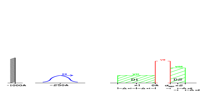
Figure 1: Simulation situation

Let us consider the situation in one dimension (Fig. 1), the potential is given by

$$V(x)=\left\{\begin{array}[]{r@{\quad:\quad}l}V_{0}&0\leq x\leq d_{POT}\\ 0&\mbox{otherwise}\end{array}\right.$$ (17)

$d_{POT}$ being the width of the barrier.

A detector $D_{1}$ is put in front of the barrier which can detect the particle without destroying it. A second detector $D_{2}$ should be put behind the barrier.

At the beginning only the detector $D_{1}$ is active. When it detects the particle at a time $t_{0}$, it turns on the detector $D_{2}$ while keeping itself turned on. So the particle must be detected first by $D_{1}$ (the possibility, that $D_{2}$ detects the particle before $D_{1}$ is therefore avoided). Thus the particle can be detected a second time by the detector $D_{1}$ or the detector $D_{2}$. If the detector $D_{1}$ detects the particle a second time at time $t_{1}$, the time difference $t_{1}-t_{0}$ is defined as the reflection time $t_{REF}$. If the particle is detected by the detector $D_{2}$ at a time $t_{2}$, then the time difference $t_{2}-t_{0}$ is by definition the traversal time $t_{TRA}$.

Another possibility is, that the particle is never detected or is detected only once. Therefore the experiment or simulation should be stopped after a finite time $t_{CUT}$. The above definitions of the traversal and reflection times are of course positive and real.

A single run of the above experiment can be simulated by using the PDP-algorithm of the EEQT (more details can be found in [29]). Making a lot of runs, the mean reflection time $\tau_{R,SIM}$ is given by averaging all runs which result in a reflection time $t_{REF}$ and the mean traversal time $\tau_{T,SIM}$ is given by averaging all times of runs, which yield a traversal time $t_{TRA}$.

There exist many other approaches for calculating mean traversal and reflection times of the interval $[x_{1},x_{2}]$ between the centers of the two detectors (for a review see for example [30, 31, 32]).

One of these are the phase time introduced by Hartman [33], which is similar to following the peak of the wave packet or the ”semi-classical” time, which is derived out of the classical expressions.

Another possibility is to install an infinitesimally small magnetic field in the range $[x_{1},x_{2}]$ and look at the rotation angle of the electron spin, this is the idea of the Büttiker-Larmor traversal time derived by Büttiker [34].

In the Bohm trajectory approach, one can talk about trajectories of particles and therefore there exists a clear definition of traversal and reflection times (for example see [35, 36, 37, 38, 39]).

The mean reflection time $\tau_{R,SIM}$ computed by the PDP-algorithm of the EEQT is compared which the results of the above approaches (the exact formulas of the results in the other approaches can be found in [29]).

One result is, that the mean reflection time $\tau_{R,SIM}$ is mostly smaller than those of the other approaches(Fig. 2). The reason is that the first detector cannot distinguish whether the particle is traveling toward the barrier, or is returning from the barrier, when it is detected a second time. So reflection times of particles, which do not reach the barrier, are also measured.

Another question is: how the mean traversal time $\tau_{T,SIM}$ depends on the barrier length. The phase time results for plane waves are independent of the barrier length. This fact is called the ”Hartman-effect”. This effect was also seen in experiments with photons (for example the experiments done by Enders and Nimtz [40, 41, 42], done by Steinberg, Kwiat and Chiao [43] and done by Spielmann, Szipöcs, Stingl and Krausz [44]).

Here electrons are used and an additional detector is put before the barrier in contrast to the photon-experiments. The question then is, whether there is still a ”Hartman-effect” or if there is no such effect due to the fact of the additional detector.

In our simulations, the energy of the particle, the height of the barrier, and the detector parameters are fixed and the barrier length $d_{POT}$ is varied (Fig. 3(a)).

The simulated times $\tau_{T,SIM}$ grow with increasing barrier width $d_{POT}\geq 3\mbox{\AA}$. With these detectors the simulation shows no wider range of barrier width with constant traversal times, and therefore no ”Hartman-effect”.

The simulation results and the Larmor clock results for plane waves show qualitatively the same characteristic: nearly the same linear growth with increasing barrier width.

Another result is: how the mean traversal time depends on the barrier height for very wide barriers (Fig. 3(b)).

The simulated times $\tau_{T,SIM}$ show a maximum if the barrier height equals the energy of the incident wave packet, i.e. $V_{0}\approx E_{0}$. For higher barriers the traversal time becomes smaller; smaller than the traversal time without barrier.

This fact can be interpreted in this way: that the mean “velocity” of the electron is greater in the case of a very high and wide barrier than in the case of a free particle. But we must remember, that up to now the formalism is non-relativistic and a relativistic formalism would perhaps give different results.

The Büttiker Larmor approach and the “semi-classical” approach show in the ranges $V_{0}<3eV$ and $V_{0}>11eV$ qualitatively the same behavior as our simulation: the traversal times decrease for increasing barrier height and are also smaller for very high barriers than the time without barrier.

Moreover there is a dependence between the traversal and reflection times and the detector parameter. The probability of an ideal measurement in the standard theory of Quantum Mechanics does not depend on the detector as these are only measurements of an infinitesimal duration. For continues measurements, such a dependence is not surprising.

5 Quantum Chaos and Quantum Fractals

When we speak about ”chaos,” we usually mean instability in the motion of most classical systems; that is, system behavior that depends so sensitively on the system’s precise initial conditions that it is, in effect, unpredictable and cannot be distinguished from a random process. This kind of behavior is not to be expected in quantum systems, essentially, for two different, yet related, reasons. The first of these is that quantum evolution equations are linear; and the second is that Heisenberg’s indeterminacy smoothes out subtle intricacies of classical chaotic orbits. The result is that there are several different approaches to ”quantum chaos”. One approach is to study the dynamics of quantum systems which are classically chaotic; that is to study non-stationary states. Another approach is to look at stationary states and concentrate on the form of the wave function (or its Wigner distribution function). Yet another approach is to concentrate on energies of stationary states, and how the distribution of quantum energy eigenvalues reflects the chaos of the classical trajectories (cf. [45]). Finally one can discuss the problem of algorithmic inaccessability of certain quantum mechanical states [46].

The quantum chaos that we want to study has nothing to do with any of the above. It is a new category, and it arose naturally out of our approach to the quantum measurement problem. According to our definition: Quantum Chaos is the chaotic behavior of quantum jumps and accompanied readings of classical instruments in a particular class of experiments, namely when experiments are set so as to perform a simultaneous, continuous, fuzzy measurement of several incompatible (i.e. incommeasurable, or noncommuting) observables. This kind of behavior is easily modeled in EEQT, as EEQT is the only theory (even if only semi-phenomenological) that provides ways of simple mathematical modeling of ”experiments” and ”measurements” on single quantum systems.

The example we present here, modeling measurement of spin simultaneously in four different directions, was first introduced in an unpublished report [47] by one of us (AJ), and then given as a subject of PhD thesis to G. Jastrzebski [48].

Before we describe the model, and the resulting chaotic behavior and strange attractor on quantum state space, let us make first a comment about the very question of simultaneous measurability of noncommuting observables. This subject has become quite controversial since the early formulation of Heisenberg’s uncertainty relations. Mathematically these relations are precise and leave no doubt about their validity. But, the question of how to interpret them physically and philosophically, has become a subject of hot discussions. To quote from Popper’s ”Unended Quest” [49]:

”The Heisenberg formula do not refer to measurements; which implies that the whole current ”quantum theory of measurement” is packed with misinterpretations. Measurements which according to the usual interpretation of the Heisenberg formulae are ”forbidden” are according to my results not only allowed, but actually required for testing these very formulae.”

Hilary Putnam came to a similar conclusion [50]:

”Recently I have observed that it follows from just the quantum mechanical criterion for measurement itself that the ”minority view” is right to at least the following extent: simultaneous measurements of incompatible observables can be made . That such measurement cannot have ”predictive value” is true …”

These words, written almost twenty years ago, suggest to us that there is some chaotic behavior involved, and that this chaos and its characteristics ought to be studied, both theoretically and experimentally. Yet, for some reason, either no one noticed, or they were not interested in looking into the problem quantitatively. We need to ask why? Perhaps for the very same reason that no one has been paying attention to the fact that events do occur. To quote from Tom Phipps’ ”Heretical Verities”, where he describes the publication of his paper ”Do Quantum Events Occur” in IEEE Journal:

”Recognizing that physics and physicists were dead, I thought to determine if electrical engineers were more alive. The answer was no . I am currently considering appealing the matter to an unbiased audience of farmers … ”

Our present point of view on quantum events is rather similar to that advocated by Phipps over twelve years ago. But, one needs more than a point of view, and, fortunately, we also have a precise mathematical model to deal with the subject in a quantitative way.

5.1 Tetrahedral spin model

The model was constructed to be as simple as possible, and yet interesting. The simplest quantum system is spin $1/2$, which can be oriented toward any point on a sphere. Mathematically we are dealing with Hilbert space ${\bf C}^{2}$ of two complex dimensions. Quantum states are rays in this space, thus elements of the projective plane $P{\bf C}^{2}$, which is isomorphic to two-dimensional sphere $S^{2}$. Equivalently, each quantum spin state can be thought of as being an eigenstate of spin operator $\vec{\sigma}\cdot\vec{n}$ along some direction $\vec{n}$. To get a simple and yet interesting behavior, we will couple our quantum spin to four yes-no classical devices that are designed so as to make fuzzy measurements of spin direction in four different space directions simultaneously (and, it is no wonder that the resulting behavior of our system will be, as we will soon see, somewhat schizophrenic!).

Why did we take four spin directions rather than two or three?

Well, for simplicity we want our directions to be symmetrically distributed. Two directions would point to south and north poles of the sphere, and spin components along these directions commute - thus no chaos.

Three symmetrically distributed directions would have to be distributed along the equator, thus producing essentially one-dimensional attractor.

The simplest symmetric figure that uses all of three-dimensional freedom, and thus produces an interesting two-dimensional attractor, is a tetrahedron! And so we choose four unit vectors ${\vec{n}_{i}}$, $i=\,1,...,4$, arranged at the vertices of a regular tetrahedron

$$\vec{n}_{1}\;=\;(1,\,0,\,0),\;\;\vec{n}_{2}\;=\;(-\frac{1}{3},\,0,\,\frac{2\sqrt{2}}{3})$$

$$\vec{n}_{3}\;=\;(-\frac{1}{3},\,\sqrt{\frac{2}{3}},\,-\frac{\sqrt{2}}{3}),\;\;\vec{n}_{4}\;=\;(-\frac{1}{3},\,-\sqrt{\frac{2}{3}},\,-\frac{\sqrt{2}}{3})$$

Details of the dynamics of our model has been described elsewhere [51]. Here we will describe only the resulting non-linear iterated function system, with point dependent probabilities. The four nonlinear transformations acting on a point $\vec{r}$ on the sphere are

$$T_{i}:\vec{r}\mapsto\vec{r}_{i}\;=\;\frac{(1\>-\>\alpha^{2})\vec{r}\>+\>2\alpha(1\>+\>\alpha\vec{r}\cdot\vec{n}_{i})\vec{n}_{i}}{1\>+\>\alpha^{2}\>+\>2\alpha\vec{r}\cdot\vec{n}_{i}},\,\,\,i=1,\ldots,4\;,$$

where $0<\alpha<1$ is a fuzziness parameter (in the limit $\alpha=1$ the measurements are sharp). At each step transformations $T_{i}$ are chosen with point dependent probabilities:

$$p_{i}(\vec{r})\;=\;\frac{1\>+\>\alpha^{2}\>+\>2\alpha\vec{r}\cdot\vec{n}_{i}}{4(1\>+\>\alpha^{2})}.$$

Using the above formulas it is easy to check that each $T_{i}$ indeed maps unit sphere onto itself, that is that if $\vec{r}^{2}=1$ then also $T_{i}(\vec{r})=1$, and also that $p_{1}+\ldots+p_{4}=1\ .$ Moreover, each $T_{i}$ is one-one.

Computer simulations show that the resulting iterated function system has a strange attractor whose fractal dimension decreases from $1.44$ to $0.49$ when $alpha$ increases from $0.75$ to $0.95$ [48].

It should be noted that our iterated function system is not quite of the usual type. Our maps $T_{i}$ are not contractions - $T_{i}$ contracts around the direction $\vec{n}_{i}$, but acts as an expansion at the opposite pole. Therefore the form of point-dependent probabilities $p_{i}$ is important for convergence of the iteration process.

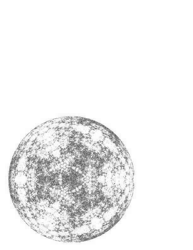
Figure 4: Tetrahedral Quantum Fractal: Quantum state trajectory for $\alpha=0.7$, $1000000000$ jumps.

There are two ways to visualize the attractor. The most evident one, widely used for iterated function systems with contractive affine maps, is to use the iteration process applied to some initial vector $\vec{r}$. Fig. 4 gives an illustration of this method applied to our case. But, because of the fact that the maps $T_{i}$ are, in our case, one-to-one and onto, we can apply here another method, that is not applicable for affine iterated function systems. This other method consists of iterations of the associated Markov operator $P$ applied to some initial measure. Invertibility of transformations $T_{i}$ assures then that if the initial measure $\mu_{0}$ is Lebesgue continuous, then all $\mu_{n}=P^{n}(\mu_{0})$ are also Lebesgue continuous, and thus can be easily visualized as functions $\mu_{0}(x)$ and $\mu_{n}(x)$ respectively.

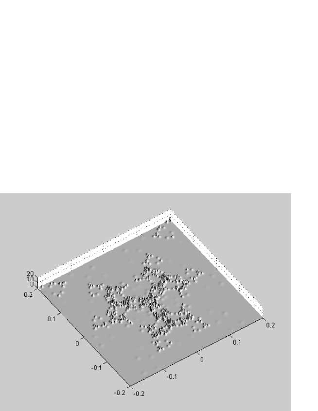
Figure 6: Tetrahedral Quantum Fractal: $\alpha=0.7$, $5\times$zoom shows self-similarity. $Log(1+\mu_{7}(x)$ on the vertical scale.

Fig. 5 show 8th iteration of the Markov operator applied to the invariant measure on the sphere (plane view of the upper hemisphere), while Fig. 6, shows $5\times$ zoom of the 7th iteration .

6 Concluding remarks

In the foregoing examples, we have seen that EEQT is, indeed, an enhancement of the standard quantum formalism, for the most important reason that it allows us to discuss, in a quantitative way, topics that are not easily treated within the orthodox approach: time series of events generated by individual quantum systems, generation of cloud chamber tracks, tunneling times, simultaneous measurement of non-commuting observables, back-action of classical variables on a quantum system, etc. EEQT can also provide an engine powering Everett-Wheeler many-world branching-tree.

In spite of all of these advantages and useful maneuvers, these practical applications, EEQT is still not a fully developed fundamental theory; though we are working in this direction. One of the arbitrary factors we have to deal with is that the coupling operators $g_{\alpha\beta}$ have to be cooked up in each case. In simple cases, like those discussed in the present paper their choice is rather unproblematic, yet even then we are not quite happy with justification of this rather than another choice. One possible way out would be to adhere to the often expressed point of view that all measurements can be, in a final instant, reduced to position measurements. Then, we can try to reduce every position measurement to sharp Dirac delta-function detectors. Yet, even then, we are left with an arbitrary value of a coupling constant for each of the point detectors. This arbitrariness, although not so much of a problem in practical applications of EEQT (for instance, as shown in Ref. [52] , for a wide range of values of the coupling constant, change of its value affects only the overall normalization constant), yet it makes us wonder about the iceberg floating beneath the tip of EEQT that we DO see?

Frankly speaking we do not know. But, from all we do know, we can speculate about possible future evolution of EEQT. This speculation goes back more than ten years, to a paper by one of us [53], a paper which set up the program of which EEQT is a partial realization. Quoting from this paper:

The theory, the main idea of which we have just sketched, must include into its scope two extremely different realities: the classical world and the quantum world. Or, making the division in a different direction: the world of matter, and the world of information. However, the differences between these two aspects of reality are so great, that their unification seems to be impossible without a ”catalyst”, and we guess that this catalyst is light. (…) Coherent infra-red photon states lead to continuous superselection rules or, in other words, algebra of observables of the photon field has a non-trivial center, whose elements parameterize infra-red representations. (…) Classical information is coded into the shape of infra-red photon cloud.

Thus one of our future projects is deriving EEQT from quantum electrodynamics, where the classical parameter enters naturally as the index of inequivalent non-Fock infrared representations. We believe that using infinite tensor product representations of quantum systems with an infinite number of degrees of freedom, we will arrive naturally at our $g_{\alpha}\beta$ operators relating to Hilbert spaces of inequivalent representations of CCRCAR.

Acknowledgments One of us (A.J) would like to thank L.K-Jadczyk for invaluable help.

Figure 2: Mean reflection time versus particle energy $E_{0}$

simulation parameters: initial wave packet: $x_{0}=-250\mbox{\AA}$, $\eta=25\mbox{\AA}$, barrier: $d_{POT}=5\mbox{\AA}$, $V_{0}=10eV$, detector $D_{1}$: $x_{1}=-25\mbox{\AA}$, $\Delta x_{1}=25\mbox{\AA}$, $W_{01}=0.16eV$, detector $D_{2}$: $x_{2}=10\mbox{\AA}$, $\Delta x_{2}=5\mbox{\AA}$, $W_{02}=2.56eV$;

mean reflection time $\tau_{SIM,R}$ (solid line with circles and errorbars);

phase time approach : wave packet (dotted line);

“semi-classical” reflection time : wave packet (dashed-dotted line);

Bohm trajectory approach (boxes with dashed line)

Figure 3: Mean traversal time

simulation situation: initial wave packet: $E_{0}=5eV$, $x_{0}=-250\mbox{\AA}$, $\eta=12.5\mbox{\AA}$, detector $D_{1}$: $x_{1}=-12.5\mbox{\AA}$, $\Delta x_{1}=12.5\mbox{\AA}$, $W_{01}=0.16eV$, detector $D_{2}$: $x_{2}=d_{POT}+5\mbox{\AA}$, $\Delta x_{2}=5\mbox{\AA}$, $W_{02}=2.56eV$,

mean traversal time $\tau_{SIM,T}$ (solid line with circles and errorbars);

phase time approach: plane wave (crosses), wave packet (dotted line);

“semi-classical” traversal time: wave packet (dashed-dotted line);

Büttiker Larmor Time: plane wave (triangles), wave packet (small-dashed line);

Bohm Trajectory approach (boxes with dashed line)

(a) versus barrier width $d_{POT}$, $V_{0}=10eV$

(b) versus barrier height $V_{0}$, $d_{POT}=40\mbox{\AA}$

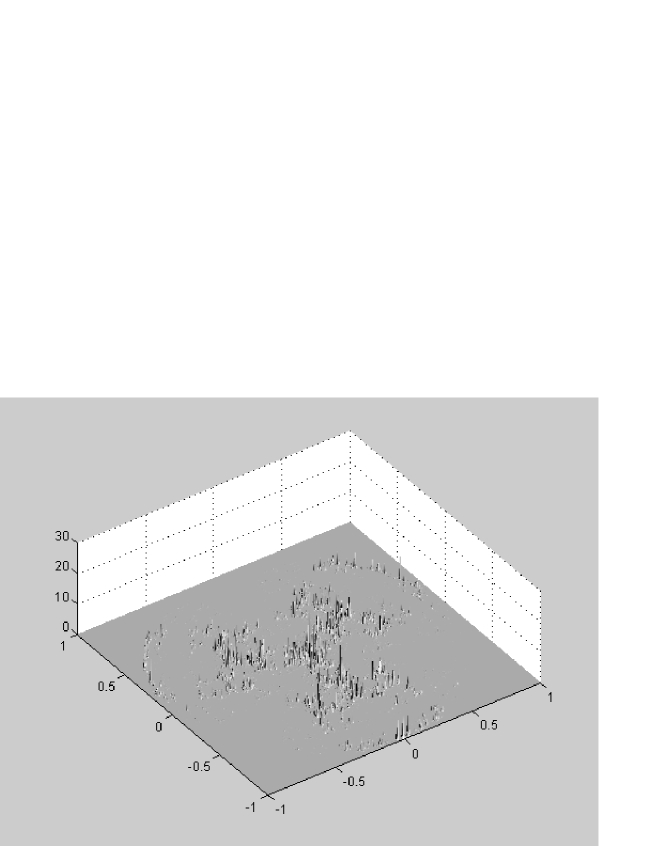
Figure 5: Tetrahedral Quantum Fractal: $\alpha=0.7$, Approximation to the strange attractor. $8$th power of the Markov operator applied to the uniform measure. Plane view of the upper hemisphere. $Log(1+\mu_{8}(x))$ on the vertical scale.

References

- [1] Bell, J.: ”Towards an exact quantum mechanics” , in Theory in Contemporary Physics II. Essays in Honor of Julian Schwinger’s 70th birthday, S. Deser and R.J. Finkelstein eds., World Scientific (1989) Singapore
- [2] Bell, J. : ”Against measurement” , in Sixty-Two Years of Uncertainty. Historical, Philosophical and Physical Inquiries into the Foundations of Quantum Mechanics, Proceedings of a NATO Advanced Study Institute, August 5-15, Erice, Ed. Arthur I. Miller, NATO ASI Series B vol. 226 , Plenum Press, New York 1990
- [3] Ghirardi, G.C., Rimini, A. and Weber, T. : ”An Attempt at a Unified Description of Microscopic and Macroscopic Systems”, in Fundamental Aspects of Quantum Theory, Proc. NATO Adv. Res. Workshop, Como, Sept. 2–7, 1985, Eds. Vittorio Gorini and Alberto Frigerio, NATO ASI Series B 144, Plenum Press, New York 1986, pp. 57–64 s
- [4] Blanchard, Ph., and Jadczyk, A.: ”On the interaction between classical and quantum systems”, Phys. Lett. A 175 (1993) 157–164.
- [5] Blanchard, Ph., and Jadczyk, A.: ”Event Enhanced Quantum Theory and piecewise deterministic dynamics”, Ann. der Physik 4 (1995) 583–599.
- [6] Blanchard, Ph., and Jadczyk, A.: ”Event and piecewise deterministic dynamics in event enhanced quantum theory” , Phys. Lett. A 203 (1995) 260–266.
- [7] Landsman, N. P. : ”Algebraic theory of superselection sectors and the measurement problem in quantum mechanics”, Int. J. Mod. Phys. A6 (1991), 5349–5371
- [8] Jadczyk, A.: ”Topics in Quantum Dynamics”, in Infinite Dimensional Geometry, Noncommutative Geometry, Operator Algebras and Fundamental Interactions, pp. 59–93, ed. R.Coquereaux et al., World Scientific, Singapore 1995, hep–th 9406204
- [9] Jauch, J.M.: ”The problem of measurement in quantum mechanics” , Helv. Phys. Acta 37 (1964) 293–316
- [10] Hepp, K.: ”Quantum Theory of Measurement and Macroscopic Observables”, Helv. Phys. Acta 45 (1972), 237-248
- [11] Piron, C.: Foundation of Quantum Physics, W.A. Benjamin, Reading Mass. (1976)
- [12] Piron, C.: ”New Quantum Mechanics”, in Old and New Questions in Physics, Cosmology, Philosophy, and Theoretical Biology: Essays in Honor of Wolfgang Yourgrau, Ed. Alvyn van der Merwe, Plenum Press, New York 1983
- [13] Piron, C.: ”What Is Wrong in Orthodox Quantum Theory”, in Mathematical Problems in Theoretical Physics, Proceedings, Berlin (West) 1981, LNP 153, Springer Verlag, Berlin 1982
- [14] Gisin, N. and Piron, C.: ”Collapse of the wave packet without mixture”, Lett. Math. Phys. 5 (1981), 379-385
- [15] Gisin, N.: ”Quantum measurements and stochastic processes”, Phys. Rev. Lett. 52 (1984), 1657-1660 and 53 (1984), 1776
- [16] Araki, H.: ”A Continuous Superselection Rule as a Model of Classical Measuring Apparatus in Quantum Mechanics” , in Fundamental Aspects of Quantum Theory, (Como 1985), Ed. V. Gorini and A. Frigerio, NATO ASI Series 144, Plenum Press, New York 1986
- [17] Primas, H.: Chemistry, Quantum Mechanics and Reductionism: Perspectives in Theoretical Chemistry, Springer Verlag, Berlin 1981
- [18] Primas, H.: ”The Measurement Process in the Individual Interpretation of Quantum Mechanics”, in The Measurement Problem of Quantum Theory, Ed. M.Cini and J.M. Lévy-Leblond, IOP Publ. Ldt. Bristol, 1990
- [19] Davis, M.H.A.: Lectures on stochastic control and nonlinear filtering, Tata Institute of Fundamental Research, Springer 1984.
- [20] Davis, M.H.A.: Markov models and optimization, Monographs on Statistics and Applied Probability, Chapman and Hall, London (1992)
- [21] Jadczyk, A., Kondrat, G. and Olkiewicz, R. : ”On uniqueness of the jump process in quantum measurement theory” , J. Phys. A 30 (1996) 1-18, available from quant-ph/9512002
- [22] Haag, R.: Local Quantum Physics, 2nd ed (1996) Chap. VII: Principles and Lessons of Quantum Physics. A Review of Interpretations, Mathematical Formalism and Perspective, Springer
- [23] Omnes, R.: Understanding Quantum Mechanics, Princeton University Press (1999)
- [24] Zurek, W.: ”Decoherence, einselection and the existential interpretation (the rough guide)”, Phil. Trans. R. Soc. London A 356, 1793–1821 (1998).
- [25] Blanchard, Ph. and Jadczyk, A.: ”How and When Quantum Phenomena Become Real” , in Proc. Third Max Born Symp. Stochasticity and Quantum Chaos, Sobotka 1993, pp. 13–31, Eds. Z. Haba et all. , Kluwer Publ. 1994
- [26] Jadczyk, A.: ”Particle Tracks, Events and Quantum Theory”, Progr. Theor. Phys. 93 (1995) 631–646, available from hep-th/9407157
- [27] Jadczyk, A.: ”On Quantum Jumps, Events and Spontaneous Localization Models”, Found. Phys. 25 1995)743–762, available from hep-th/9408020
- [28] J.P. Palao, J.P. Muga, S. Brouard, and A. Jadczyk. Phys. Lett. A 233 (1997) 227.
- [29] A. Ruschhaupt. Simulations of barrier traversal and reflection times based on event enhanced quantum theory. Phys. Lett. A 250 (1998) 249-256.
- [30] E.H. Hauge and J.A. Støvneng. Tunneling times: a critical review. Rev. Mod. Phys. 61 (1989) 917.
- [31] R. Landauer and Th. Martin. Barrier interaction time in tunneling. Reviews of Modern Physics 66 (1994) 217.
- [32] G. Nimtz and H. Winfried. Prog. Quant. Electr. 21 (1997) 81.
- [33] T.E. Hartman. Tunneling of a wave packet. J. Appl. Phys. 33 (1962) 3427.
- [34] M. Büttiker. Larmor precession and the traversal time for tunneling. Phys. Rev. B 27 (1983) 6178.
- [35] C.R. Leavens. Transmission, reflection and dwell times within Bohm’s causal interpretation of quantum mechanincs. Solid State Comm. 74 (1990) 923.
- [36] C.R. Leavens. Traversal times for rectangular barrier within Bohm’s causal interpretation of quantum mechanics. Solid State Comm. 76 (1990) 253.
- [37] C.R. Leavens. Bohm trajectory and Feynman path approaches to the ”tunneling time problem”. Foundation of Physics 25 (1995) 229.
- [38] C.R. Leavens. Phys. Lett. A 197 (1995) 88.
- [39] X. Oriols, F. Martín, and J. Suñé. Phys. Rev. A 54 (1996) 2594.
- [40] A. Enders and G. Nimtz. On superluminal barrier traversal. J. Phys. I France 2 (1992) 1693-1698.
- [41] A. Enders and G. Nimtz. Zero-time tunneling of evanescent mode packets. J. Phys. I France 3 (1993) 1089-1092.
- [42] A. Enders and G. Nimtz. Evanescent-mode propagation and quantum tunneling. Phys. Rev. E 48 (1993) 632-634.
- [43] A.M. Steinberg, P.G. Kwiat, and R.Y. Chiao. Measurement of the single-photon tunneling time. Phys. Rev. Lett. 71 (1993) 708-711.
- [44] Ch. Spielmann, R. Szipöcs, A. Stingl, and F. Krausz. Tunneling of optical pulses through photonic band gaps. Phys. Rev. Lett. 73 (1994) 2308-2311.
- [45] Berry, M.: ”Semiclassical Chaology”, in Quantum Measurement and Chaos, NATO ASI Series 161, ed. E.R. Pike and Sarben Sarkar, Plenum, New York 1986
- [46] Peres, A.: ”Quantum Chaos and the Measurement Problem”, as in Ref. [45]
- [47] Jadczyk, A.: ”IFS Signatures of Quantum States”, IFT Uni Wroclaw, internal report, September 1993.
- [48] Jastrzebski G., ”Interacting classical and quantum systems. Chaos from quantum measurements”, Ph. D. thesis, University of Wrocław (in Polish), 1996
- [49] Popper, K.: Unended Quest. An intellectual Autobiography, Routledge, London 1993
- [50] Putnam, H.: ”Quantum Mechanics and the Observer” , Erkenntnis 16, 1981
- [51] Blanchard, Ph., Jadczyk, A., and Olkiewicz, R.: ”Completely Mixing Quantum Open Systems and Quantum Fractals” , e-print archive quant-ph/9909085
- [52] Blanchard, Ph., Jadczyk, A.: ”Time of Events in Quantum Theory” , Helv. Phys. Acta 69 (1996) 613–635, also available as quant-ph/9602010,
- [53] Jadczyk, A.: ”Bioelectronics as viewed by a theoretical physicist” - in Polish, BIOELEKTRONIKA MATERIA Y VI SYMPOZJUM, Katolicki Uniwersytet Lubelski, 20-21 XI 1987, W. Sedlak, J. Zon, M. Wnuk (ed.) Redakcja Wydawnictw KUL, Lublin 1990; also available online at URL: http://www.cassioapea.org/quantum_future/biopl1.htm